Lattice Boltzmann Method Simulation of Bubble Dynamics for Enhanced Boiling Heat Transfer by Pulsed Electric Fields

Abstract

The application of electric fields during pool boiling heat transfer has demonstrated significant potential to enhance thermal performance. However, research on boiling heat transfer enhancement under pulsed electric fields remains insufficient. To further improve pool boiling efficiency, this study systematically investigates the effects of pulsed electric fields, uniform electric fields, and electric field-free conditions on heat transfer performance using the Lattice Boltzmann Method (LBM). The results show that, compared with the uniform electric field and electric field-free condition, the pulsed electric field resulted in the smallest bubble detachment diameter and detachment period, with a higher heat flux density on the wall and the best heat transfer enhancement effect. Under the pulsed electric field, the electric force undergoes abrupt changes at the beginning and end of each pulse peak, exerting greater compression on the bubble base. Simultaneously, this leads to accelerated gas rise inside the bubble, bubble stretching, and contraction of the bottom phase boundary. There exists an optimal pulse frequency that minimizes the bubble detachment period and diameter, resulting in the best wall heat transfer enhancement effect. The effective areas for enhanced boiling heat transfer by pulsed electric fields are the bubble base and the “V”-shaped region connected to the bubble bottom.

1. Introduction

In recent years, enhanced heat transfer in pool boiling has been one of the hottest research topics. Methods for enhancing pool boiling heat transfer can be broadly categorized into two categories based on the enhancement technique: (1) passive enhancement methods, represented by improved surface structures [1] and surface wettability [2]; and (2) active enhancement methods, represented by externally applied acoustic fields [3,4] and electric fields [5,6,7]. Among these, the application of an electric field to the heated surface significantly influences bubble nucleation and dynamics. J. Madadnia et al. [8] investigated the influence of an electric field on the heat transfer characteristics during single bubble boiling and found that both the bubble detachment period and bubble detachment diameter decreased under the influence of an electric field. Similar phenomena were also observed in experiments by S. W. Ahmad et al. [9] and H. Chang et al. [10]. Y. Hristov et al. [11] experimentally investigated the influence of an electric field on pool boiling heat transfer performance on a smooth surface and found that the application of an electric field increased the saturation pool boiling heat transfer coefficient. However, different electrode configurations led to different electric field distributions, which in turn had a significant impact on the experimental results. Yanjun Chen et al. [12] investigated the influence of an electric field with periodically changing directions on pool boiling heat transfer. Their findings revealed that, when compared with a uniform electric field, this periodically alternating electric field promoted the rewetting process of the wall drying zone, accelerated bubble detachment, and enhanced the overall pool boiling heat transfer performance. Due to the instantaneous nature and complexity of boiling heat transfer, combined with the invisibility of electric field distribution, there are certain limitations and instabilities in pool boiling experimental data collection and accurate electric field arrangement. Therefore, many scholars have dedicated themselves to the development and research of numerical simulation models. Among them, owing to its inherent accuracy in modeling interfacial dynamics and numerical stability across complex flow regimes, the Lattice Boltzmann Method (LBM) has been developed rapidly in the study of two-phase flows [13,14,15,16,17]. Yuan Feng et al. [6] used a two-dimensional LBM coupled with a boiling model and an electric field model to simulate single-bubble pool boiling on a wall with a non-uniform electric field applied. The results showed that the application of an electric field changed the forces acting on the bubble, stretching it under the action of the electric force. The electric field reduced the bubble detachment diameter and period. Zhang Sen et al. [18] conducted a quantitative analysis of nucleate boiling on a cone-fin surface under an electric field through two-dimensional Lattice Boltzmann simulations and found that the application of an electric field increased the heat flux of boiling heat transfer on the cone-fin surface. Li et al. [19] used a two-dimensional LBM to study the enhancement mechanism of electric fields on boiling heat transfer in pillar structures and found that the combination of micropillar surface structures and externally applied electric fields can produce a synergistic effect, significantly enhancing boiling heat transfer efficiency.

Currently, most research on electric field-enhanced pool boiling heat transfer is based on a constant uniform electric field, and there are few reports on bubble dynamics and boiling heat transfer performance in pool boiling under a pulsed non-uniform electric field. Therefore, based on a two-dimensional LBM, this paper couples the pseudo-potential two-phase flow model and the ideal dielectric model to investigate the enhanced heat transfer process in pool boiling under pulsed square wave electric field excitation. It examines the bubble dynamics behavior in different electric fields and the influence of pulse frequency on bubble detachment behavior, revealing the mechanism of pulsed electric field-enhanced boiling heat transfer.

2. Numerical Methods

2.1. Lattice Boltzmann Pseudopotential Model

The pseudopotential LB model was first proposed by Shan and Chen [15,16]. The distribution function evolution equation of the single-component D2Q9 pseudopotential LB model can be written as:

$$\begin{array}{l}{f}_{\mathrm{i}}\left(x+e_{\mathrm{i}}{\delta }_{\mathrm{t}},t+{\delta }_{\mathrm{t}}\right)-f_{\mathrm{i}}(x,t)=-{\displaystyle \frac{1}{\tau }}\left(f_{\mathrm{i}}(x,t)-f_{\mathrm{i}}^{\mathrm{eq}}(x,t)\right)+\mathsf{\Delta }{f}_{\mathrm{i}}(x,t)\hfill \end{array}$$

(1)

where f_i(x,t) is the density distribution function, with i and x representing the direction and position of particles in the density distribution function, respectively, where i ∈ [0, 8], e_i is the discrete velocity, δ_t is the discrete time, and δ_t = 1.0. Δf_i(x,t) is the body force term causing changes in the distribution function, τ is the modified relaxation time [17], and f_i^eq(x,t) is the equilibrium distribution function, which is expressed as:

$$f_{\mathrm{i}}^{\mathrm{eq}}(x,t)={\omega }_{\mathrm{i}}\rho \left[1+{\displaystyle \frac{e_{\mathrm{i}}\cdot u}{c_{\mathrm{s}}^2}}+{\displaystyle \frac{{\left(e_{\mathrm{i}}\cdot u\right)}^2}{2c_{\mathrm{s}}^4}}-{\displaystyle \frac{u^2}{2c_{\mathrm{s}}^2}}\right]$$

(2)

where ρ is the fluid density, with its discrete form being ρ(x,t). ω_i is the weighting coefficient. In the D2Q9 model, when i = 0, ω_i = 4/9; when i = 1–4, ω_i = 1/9; and when i = 5–8, ω_i = 1/36. c_s is the lattice sound speed, with c_s² = c₀/3, where c₀ is the lattice velocity, and c₀ = 1.0. The expression for the body force term is:

$$\mathsf{\Delta }{f}_{\mathrm{i}}(x,t)=f_{\mathrm{i}}^{\mathrm{eq}}(\rho ,u+\mathsf{\Delta }u)-f_{\mathrm{i}}^{\mathrm{eq}}(\rho ,u)$$

(3)

where Δu is the velocity increment, with Δu = F∙δ_t/ρ. Herein, the total body force F = F_int + F_w + F_g + F_e, where F_int is the interparticle interaction force, which leads to phase transitions; F_g is the gravitational force; F_w is the interaction force between the fluid and solid; and F_e is the electric field force acting on bubbles. Their discretized expressions are respectively:

$$\begin{array}{l}{F}_{\mathrm{int}}\left(x,t\right)=-A{\displaystyle {\sum }_{\alpha =0}^{8}w\left(|e_{\mathrm{i}}{|}^2\right)}U\left(x+e_{\mathrm{i}}{\delta }_{\mathrm{t}},t\right)e_{\mathrm{i}}\\ -\left(1-A\right)G\psi \left(x,t\right){\displaystyle {\sum }_{\alpha =0}^{8}w\left(|e_{\mathrm{i}}{|}^2\right)}\psi \left(x+e_{\mathrm{i}}{\delta }_{\mathrm{t}},t\right)e_{\mathrm{i}}\end{array}$$

(4)

$$F_{\mathrm{w}}\left(x,t\right)=-\psi \left(x,t\right)G_{\mathrm{s}}{\displaystyle {\sum }_{\alpha =0}^{8}w\left(|e_{\mathrm{i}}{|}^2\right)}s\left(x+e_{\mathrm{i}}{\delta }_{\mathrm{t}}\right)e_{\mathrm{i}}$$

(5)

$$F_{\mathrm{g}}\left(x,t\right)=\left(\rho \left(x,t\right)-{\rho }_{\mathrm{ave}}\right)g$$

(6)

$$F_{\mathrm{e}}(x,t)=-{\displaystyle \frac{1}{2}}E\cdot E\nabla \epsilon {\epsilon }_0$$

(7)

where w(|e_i|²) is the weighting coefficient, A is a weight factor to improve computational stability, G is the gas–liquid interaction constant, with a value of −1, U(x + e_iδ_t,t) is the potential function between adjacent particles, ρ_ave is the average density in the computational domain, and s(x) is the indicator function for wall interaction force. When a particle is adjacent to the wall, s(x) = 1; when the particle is far from the wall, s(x) = 0. g is the gravitational acceleration and ψ(x, t) is the discretized form of the effective fluid density, which is expressed as:

$$\psi (\rho )=\sqrt{{\displaystyle \frac{2\left(p-c_{\mathrm{s}}^2\rho \right)}{c_{0}g}}}$$

(8)

The pressure p is obtained from the Peng–Robinson (P-R) equation of state [16], which is expressed as:

$$p={\displaystyle \frac{\rho RT}{1-b\rho }}-{\displaystyle \frac{a{\rho }^2\epsilon (T)}{1+2b\rho -b^2{\rho }^2}}$$

(9)

where T is the fluid temperature, ρ is the fluid density, ε(T) = [1 + 2.4859(1−$\sqrt{T/T_{\mathrm{c}}}$], T_c is the critical temperature, and the parameters in the equation are set as R = 1.0, a = 0.04, and b = 0.09 [17].

The expressions for fluid density ρ and velocity u are:

$$\rho ={\displaystyle \sum }_i{f}_{\mathrm{i}}(x,t)$$

(10)

$$\rho u={\displaystyle \sum }_i{e}_{\mathrm{i}}{f}_{\mathrm{i}}(x,t)$$

(11)

where u is the pseudo-velocity of the fluid, and the expression for the true fluid velocity U is:

$$\rho U={\displaystyle \sum }_i{e}_{\mathrm{i}}{f}_{\mathrm{i}}+{\displaystyle \frac{{\delta }_{\mathrm{t}}}{2}}F$$

(12)

2.2. Ideal Dielectric Model

According to the theory of electrohydrodynamics (EHD), the electric field force can be expressed as:

$$F_e=q_{\mathrm{v}}E-{\displaystyle \frac{1}{2}}E\cdot E\nabla {\epsilon }_0\epsilon +{\displaystyle \frac{{\epsilon }_0}{2}}\nabla \left(\rho {\displaystyle \frac{\partial \epsilon }{\partial \rho }}E\cdot E\right)$$

(13)

where ε₀ is the vacuum permittivity and ε is the permittivity at the lattice point. The first term on the right-hand side of the equation represents the Coulomb force acting on the bubble, the second term represents the dielectrophoretic force, and the third term represents the electrostrictive force. Assuming that the fluid in the computational domain is an ideal dielectric, i.e., the fluid is incompressible and does not carry charges, The first and third terms on the right-hand side of Equation (13) evaluate to zero. Therefore, F_e can be simplified to:

$$F_e=-{\displaystyle \frac{1}{2}}E\cdot E\cdot \nabla {\epsilon }_0\epsilon$$

(14)

where E is the electric field intensity, and its governing equation is ∇∙(ε₀ε E) = 0. E can be obtained from E = −∇·V, where V is the electric potential. The governing equation for the electric field can then be written as:

$$\nabla \cdot \left({\epsilon }_0\epsilon \nabla V\right)=0$$

(15)

The expression for the electric potential V is:

$$V={\displaystyle \sum }_i{\eta }_{\mathrm{i}}(x,t)$$

(16)

where η_i(x,t) is the electric potential distribution function, and its governing equation is:

$${\eta }_{\mathrm{i}}\left(x+e_{\mathrm{i}}\mathsf{\Delta }t,t+\mathsf{\Delta }t\right)-{\eta }_{\mathrm{i}}(x,t)=-{\displaystyle \frac{1}{{\tau }_{\mathrm{e}}}}\left[{\eta }_{\mathrm{i}}(x,t)-{\eta }_{\mathrm{i}}^{\mathrm{eq}}(x,t)\right]$$

(17)

In this equation, τ_e is the relaxation time for Equation (17), and its expression is τ_e = 3ε₀ε + 0.5. η_α^eq(x,t) is the equilibrium distribution function for the evolution equation of the electric potential, and its expression is:

$${\eta }_{\mathrm{i}}^{\mathrm{eq}}(x,t)=w_{\mathrm{i}}V$$

(18)

2.3. Energy Equation Model

In this paper, a single-relaxation D2Q9 heat transfer model is employed. The evolution equation for temperature distribution function is:

$$g_{\mathrm{i}}\left(x+e_{\mathrm{i}}{\delta }_{\mathrm{t}},t+{\delta }_{\mathrm{t}}\right)-g_{\mathrm{i}}(x,t)=-{\displaystyle \frac{1}{{\tau }_{\mathrm{T}}}}\left(g_{\mathrm{i}}(x,t)-g_{\mathrm{i}}^{\mathrm{eq}}(x,t)\right)+{\delta }_{\mathrm{t}}{w}_{\mathrm{i}}\varphi$$

(19)

where g_i(x, t) represents the temperature distribution function of particles, and g_i^eq is the corresponding equilibrium temperature distribution function, which is expressed as:

$$g_{\mathrm{i}}^{\mathrm{eq}}={\omega }_{\mathrm{i}}T\left[1+{\displaystyle \frac{e_{\mathrm{i}}V}{c_{\mathrm{s}}^2}}+{\displaystyle \frac{{\left(e_{\mathrm{i}}V\right)}^2}{2c_{\mathrm{s}}^4}}-{\displaystyle \frac{V^2}{2c_{\mathrm{s}}^2}}\right]$$

(20)

where τ_T is the modified relaxation time [17], and its expression is:

$${\tau }_{\mathrm{T}}={\displaystyle \frac{3}{2}}{\displaystyle \frac{\lambda }{\rho c_{\mathrm{p}}{c}^2{\delta }_{\mathrm{t}}}}+{\displaystyle \frac{1}{2}}°$$

(21)

The expression for the fluid property χ (such as fluid viscosity, thermal diffusivity or permittivity) at the liquid–vapor interface is:

$$\chi ={\chi }_{\mathrm{l}}{\displaystyle \frac{\rho -{\rho }_{\mathrm{v}}}{{\rho }_{\mathrm{l}}-{\rho }_{\mathrm{v}}}}+{\chi }_{\mathrm{v}}{\displaystyle \frac{{\rho }_{\mathrm{l}}-\rho }{{\rho }_{\mathrm{l}}-{\rho }_{\mathrm{v}}}}$$

(22)

where χ_l and χ_v represent the fluid properties of the liquid and vapor phases, respectively, while ρ_l and ρ_v represent the densities of saturated liquid and gas, respectively. ϕ in Equation (22) is the phase change source term, and its expression is:

$$\varphi =\left[T-{\displaystyle \frac{\rho h_{\lg }}{c_{\mathrm{v}}\left({\rho }_{\mathrm{l}}-{\rho }_{\mathrm{v}}\right)}}\right]\nabla \cdot V$$

(23)

where the latent heat of vaporization during the phase change process is denoted as h_lg = h_g − h_l, where h_g and h_l are the enthalpies of the gas and liquid phases, respectively, with h_g = 0.5 and h_l = 0.17. c_v represents the specific heat at constant volume. The temperature T is expressed as:

$$T={\displaystyle \sum }_i g_{\mathrm{i}}$$

(24)

Characteristic units l₀, u₀, and t₀ are introduced, and their expressions are:

$$\left\{\begin{array}{c}{l}_0=\sqrt{{\displaystyle \frac{\sigma }{g\left({\rho }_{\mathrm{l}}-{\rho }_{\mathrm{v}}\right)}}}\\ u_0=\sqrt{g{l}_0}\\ t_0={\displaystyle \frac{l_0}{u_0}}\end{array}\right.$$

(25)

Based on the principle of similarity, the conversion relationships between lattice units and physical units are:

$$\left\{\begin{array}{l}{T}^{*}={\displaystyle \frac{T^{\mathrm{lu}}}{T_{\mathrm{c}}^{\mathrm{lu}}}}={\displaystyle \frac{T^{\mathrm{pu}}}{T_{\mathrm{c}}^{\mathrm{pu}}}}\\ l^{\ast }={\displaystyle \frac{l^{\mathrm{lu}}}{l_0^{\mathrm{lu}}}}={\displaystyle \frac{l^{\mathrm{pu}}}{l_0^{\mathrm{pu}}}}\\ t^{\ast }={\displaystyle \frac{t^{\mathrm{lu}}}{t_0^{\mathrm{lu}}}}={\displaystyle \frac{t^{\mathrm{pu}}}{t_0^{\mathrm{pu}}}}\end{array}\right.$$

(26)

All the dimensions mentioned in this paper are dimensionless units derived from lattice units, namely T*, l*, and t*.

3. Computational Model and Validation

3.1. Computational Model

The computational domain for pool boiling is shown in Figure 1a, with dimensions set to L₁ × L₂ = 11.84 × 9.52. The base of the computational domain is a solid-phase region with a thickness of L₃ = 0.61, To fix the nucleation site of a single bubble, a constant-temperature heat source with a length of L₄ = 0.47 is set at the bottom center of the heating domain. To maintain nucleation boiling, the heat source temperature is set to T_h = 1.35 T_c. As shown in Figure 1a, bubbles grow and detach from the center of the wall. The morphological changes during bubble growth affect the local heat flux on the wall. To quantitatively study these changes, this paper uses the bubble aspect ratio to approximate the bubble morphology. Figure 1b illustrates the aspect ratio AR of the bubble, which is the ratio of the bubble height H to the bubble width D, i.e., AR = H/D. A larger AR indicates a more elongated bubble shape. A liquid-phase region with a height of L₅ = 4.28 on the heating plate is set as the electric field region. The upper electrode plate is grounded with a potential of zero, and the bottom heating wall is set as the high-potential lower electrode plate. An external electric field in the liquid region is achieved by inputting different potentials. In the electric field model, inputting a pulsed potential as shown in Figure 1c on the lower electrode plate can generate a square-wave pulsed electric field. The duty ratio DR of the pulsed electric field is the ratio of the duration of the input peak potential V₀ within a single pulse cycle to the duration of the entire pulse cycle, i.e., DR = t₁/t₂. The duty ratio of the pulsed electric field in this paper is 0.5. The settings of physical quantities are shown in the following

Table 1. Nomenclature.

Symbol	Description	Value (Dimensionless)
Tc	Critical temperature	0.0729
Tl	Saturation temperature	0.86 Tc
ρl	Liquid density	7.098
λl	Liquid thermal conductivity	0.34182
ρg	Saturated vapor density	0.2156
λg	Vapor thermal conductivity	0.022788
ρw	Solid density	6
λw	Solid thermal conductivity	3.0
cv	specific heat at constant volume	5.0
cpl	Liquid specific heat at constant pressure	3.385
cpv	Vapor specific heat at constant pressure	1.034
εl	Liquid dielectric constant	0.2236
εv	Vapor dielectric constant	0.1
ε0	Vacuum dielectric constant	1
Th	Heat source temperature	1.35 Tc
g	Gravitational acceleration	3.0 × 10−5

.

3.2. Model Validation

3.2.1. Validation of Young–Laplace Law

To verify the stability of the simulation results, the computational model is validated using the Young–Laplace law, which is expressed as:

$$\Delta P=\sigma /R$$

(27)

where ΔP is the pressure difference across the bubble interface, σ is the bubble surface tension, and R is the bubble radius. According to the formula, when the bubble reaches a stable state, σ remains constant, and ΔP is inversely proportional to R. The computational domain for the validation model is 4.76 × 4.76, with initial temperatures set to 0.80 T_c, 0.86 T_c, and 0.90 T_c. A static bubble is positioned at the central location of the computational domain. When the bubble reaches a stable state, the pressure difference across the bubble interface is measured, and linear fitting is performed for each set of data points. As shown in Figure 2, after the bubble stabilizes, ΔP is inversely proportional to R, indicating that the simulation results are consistent with the Young–Laplace law and the boiling heat transfer model is stable.

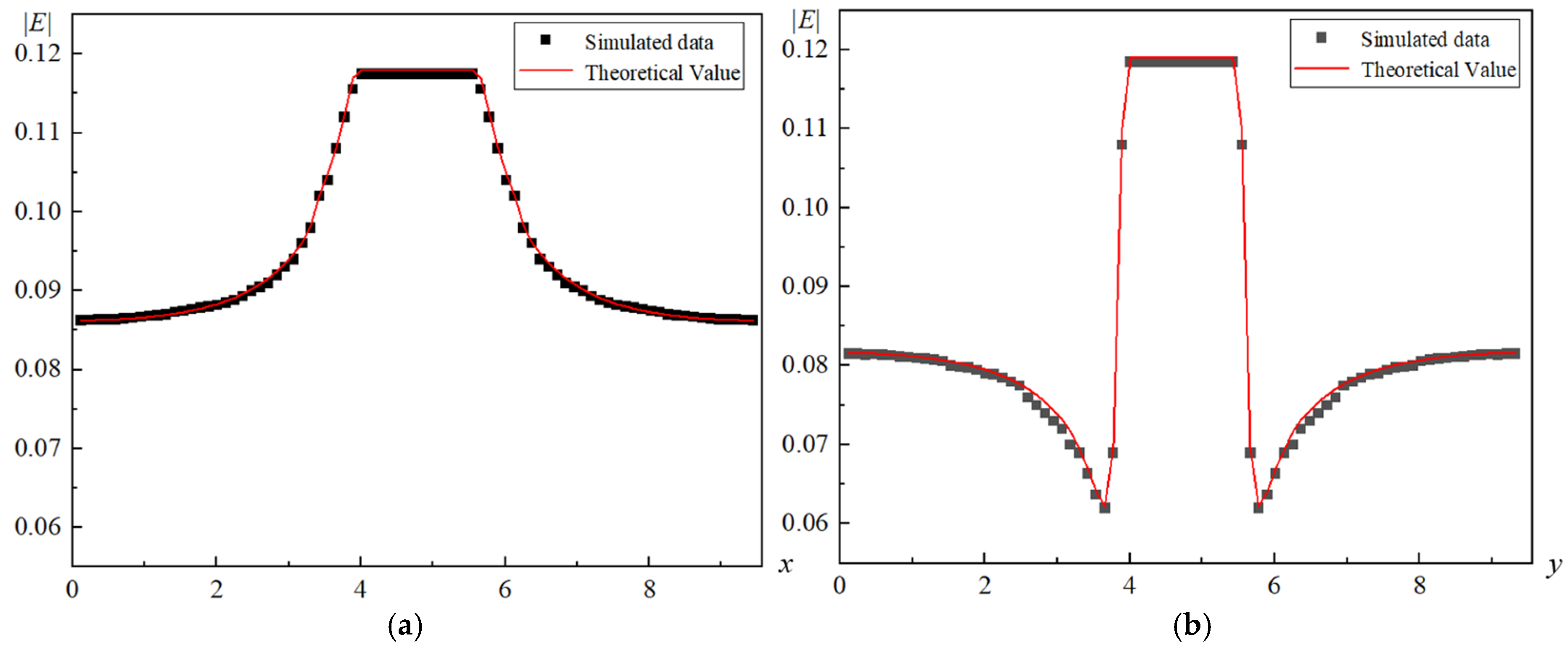
3.2.2. Validation of the Electric Field Model

To validate the accuracy of the electric field model, the validation scheme proposed by Yuan et al. [6] is adopted. A stationary bubble with a diameter of D₀ = 1.90 is placed at the center of a 9.52 × 9.52 computational domain, and a constant potential of V₀ = 17.5 is applied at the bottom of the boundary. The potential at the top of the domain is set to zero. Periodic boundaries are set at the left and right ends of the electric field model, and Zou–He boundaries are set at the top and bottom ends. Figure 3 shows the contour plot of the electric field intensity in the suspended bubble and its surrounding area under a uniform electric field. As shown in Figure 3, due to the different dielectric constants of the gas and liquid phases, the electric field intensity is higher in the gas phase and lower in the liquid phase overall. Taking the bubble center as the origin, in the x-direction, the electric field intensity decreases as x increases; in the y-direction, the electric field intensity first decreases and then increases as y increases.

Taking the bubble center as the origin, the electric field intensity around the bubble can also be derived from Equation (28) [5], which is expressed as:

$$E=\left\{\begin{array}{cc}{\displaystyle \frac{2{\epsilon }_{\mathrm{l}}{E}_0}{{\epsilon }_{\mathrm{v}}+{\epsilon }_{\mathrm{l}}}}\left(i_{\mathrm{r}}cos\theta +i_{\mathsf{\theta }}sin\theta \right),& r\le 0.5D_0\\ \begin{array}{l}\left[E_0+{\displaystyle \frac{\left({\epsilon }_{\mathrm{v}}-{\epsilon }_{\mathrm{l}}\right)D_0^2{E}_0}{4\left({\epsilon }_{\mathrm{v}}+{\epsilon }_{\mathrm{l}}\right)r^2}}\right]i_{\mathrm{r}}sin\theta \\ -\left[-E_0+{\displaystyle \frac{\left({\epsilon }_{\mathrm{v}}-{\epsilon }_{\mathrm{l}}\right)D_0^2{E}_0}{4\left({\epsilon }_{\mathrm{v}}+{\epsilon }_{\mathrm{l}}\right)r^2}}\right]i_{\mathsf{\theta }}cos\theta ,\end{array}& r>0.5D_0\end{array}\right.$$

(28)

In the equation, r is the distance from the point of interest to the center of the bubble and θ is the angle with respect to the positive x-direction. Figure 4 presents the analytical solutions of the electric field intensity at the bubble center in the x and y directions obtained from Equation (28), along with the numerical simulation results for the same directions at the bubble center as shown in Figure 3. From the figure, the simulated values are in good agreement with the theoretical predictions, thereby indicating the high accuracy of the electric field model.

4. Simulation Results and Discussion

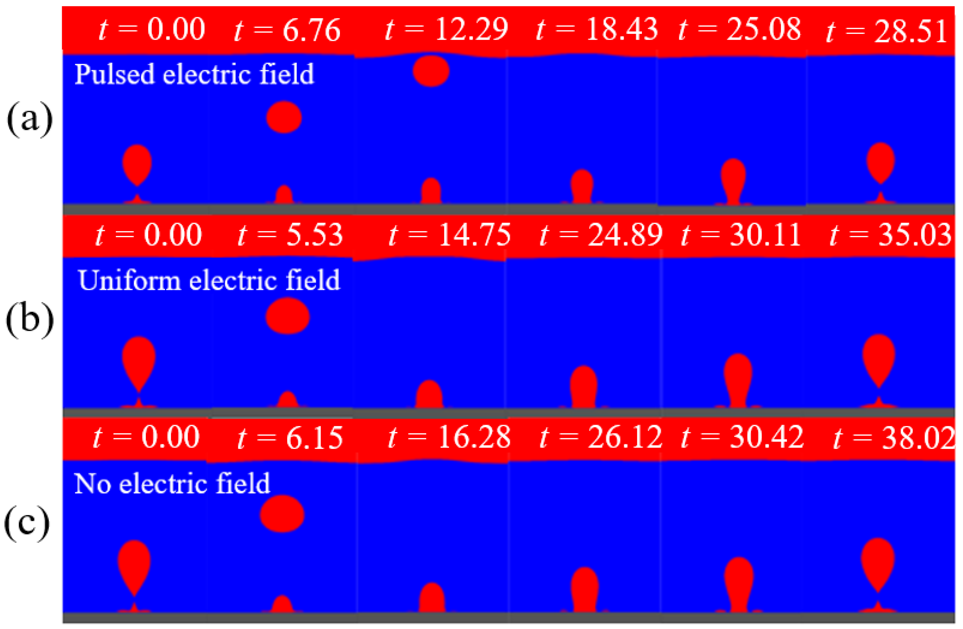
4.1. Influence of Different Types of Electric Field on Bubble Behavior

Given that various types of electric fields have an impact on bubble dynamics, three representative electric field configurations were selected for the simulation. Figure 5a–c show contour plots of bubble shapes at different time instants within one cycle in a pulsed electric field, uniform electric field, and no electric field, respectively. In the pulsed electric field, a square wave pulse potential of V₀ = 6 is applied to the lower electrode, while in the uniform electric field, a constant potential of V₀ = 6 is applied. The leftmost image in Figure 5a displays the detached bubble morphology from the previous cycle and the initial growth of a new bubble. At t = 0, the bubble from the previous cycle detaches and leaves a residual bubble on the wall. Between t = 0 and t = 6.76, the bubble rises due to buoyancy, and the residual bubble on the wall grows to form a nucleation site. Between t = 6.76 and t = 12.29, the bubble continues to grow due to wall heating, with the phase boundary expanding outward. Between t = 12.29 and t = 18.43, as the bubble grows, its height increases, and the phase boundary at the bottom of the bubble stops moving outward. As the bubble continues to grow, at t = 25.08, due to increased buoyancy, the bubble rises continuously. Under the influence of bubble surface tension, the bottom boundary of the bubble contracts inward and forms a “bubble neck.” Between t = 25.08 and t = 28.51, the “bubble neck” continues to contract inward, and the bubble starts to detach from the wall. At t = 28.51, the “bubble neck” breaks and the bubble completely detaches from the wall. The bubble growth processes under the uniform electric field and no electric field are similar (as shown in Figure 5b,c). From Figure 5, it can be concluded that the bubble detaches from the wall at t = 28.51 in the pulsed electric field, at t = 35.03 in the uniform electric field, and at t = 38.02 with no electric field. Therefore, the bubble detachment period is shortest under the pulsed electric field.

With respect to bubble morphology, the bubbles in the uniform electric field and no electric field are similar, with the uniform electric field accelerating bubble necking. Compared with the uniform electric field, the pulsed electric field makes the bubble boundary narrower, the bubble shape more slender, and the solid wall space occupied by the bubble smaller. In addition, Figure 5 shows that the diameter of the bubble when it detaches under the pulsed electric field is significantly smaller than that under the uniform electric field and with no electric field. This indicates that more bubbles with smaller diameters will be generated per unit time on the same heated wall surface. The generation and detachment of bubbles remove more wall heat, resulting in a higher heat flux density [6]. Therefore, the boiling heat transfer efficiency under the pulsed electric field is higher than that under the uniform electric field and with no electric field.

Figure 6 presents the trend of aspect ratio changes during the growth process of a single bubble in the aforementioned three electric fields. It can be observed that, as time progressed, the aspect ratio of the bubble generally increases from nucleation, growth, to detachment. However, the growth processes of the aspect ratio differ significantly under different electric fields. In the uniform electric field, the aspect ratios of the bubbles are all greater than those with no electric field. In contrast, under the square-wave pulsed electric field, the aspect ratio exhibited periodic fluctuations over time during its increase and was always greater than that under the uniform electric field. Additionally, the instantaneous aspect ratio of the bubble detaching from the wall was 1.91 under the pulsed electric field, 2.03 under the uniform electric field, and 2.20 with no electric field. This indicates that the pulsed electric field induced premature bubble necking, thereby promoting earlier detachment from the wall even at a smaller aspect ratio.

The expression for wall heat flux q* is given by:

$$q^{*}=-{\left({\displaystyle \frac{\partial T}{\partial y}}\right)}_{y=L_3}{\displaystyle \frac{\Delta y}{T_c}}°$$

(29)

where Δy is the lattice length in the y-direction. Figure 7 displays the local heat flux density distribution on the solid wall at t = 15.00 under the influence of three types of electric fields. As seen in the figure, the heat flux density displays a distribution with higher values in the central region and lower values at both lateral sides. Within the bubble, the heat flux density shows an “M”-shaped trend. The local heat flux density on the wall reached its maximum in the microlayer at the edge of the bubble. Furthermore, the wall heat flux density was highest in the pulsed electric field, followed by the uniform electric field, and lowest with no electric field, indicating that the pulsed electric field enhanced the local wall heat flux.

4.2. Influence of Electric Force on Bubble Behavior in Electric Field

To investigate the impact of pulsed electric field on bubble dynamics, the temporal variation in the electric forces acting on bubbles within a single electric field cycle was selected for simulation. Figure 8 shows contour plots of the electric force varying in response to the electric field intensity experienced by bubbles during the period from t = 18.00 to t = 21.60 in a uniform electric field with potential V₀ = 6 applied to the lower electrode and a pulsed electric field with a maximum pulse potential of V₀ = 6 and a pulse frequency of f = 6.6. According to Equation (22), the magnitude of the electric force F_e acting on the bubble was mainly determined by the dielectric constant gradient ∇εε₀ in the fluid and the magnitude of the electric field intensity |E|. As shown in Figure 8a, the electric field intensity was uniformly distributed and relatively small in the uniform electric field, and the electric force acting on the bubble was uniformly distributed along its phase boundary with a relatively small magnitude.

In contrast, Figure 8b presents a different distribution of electric field intensity and bubble-exerted electric force under the pulsed electric field and with no electric field. At t = 18.00, the previous pulse cycle ended, and since the pulsed electric field was in its trough phase at this time, the potential applied to the lower electrode was zero, and the electric field intensity within the computational domain was also zero. Consequently, the electric force exerted on the bubble was small, and its effect on the bubble was minimal. At t = 18.72, the pulsed electric field was at the beginning of the high potential phase, and the bottom of the bubble experienced a large local electric force. As time progressed, during the stage from t = 18.72 to t = 19.44, the electric field propagated toward the upper part of the bubble, while the electric field intensity near the wall gradually decreased. Starting from t = 20.16, the pulsed electric field transitioned from the peak to the trough phase, and the potential applied to the lower electrode changed from V₀ to 0. Due to the abrupt change in the electric field, the bubble base again experienced a local, short-duration high electric field intensity, while the upward-diffusing electric field began to weaken rapidly before reaching the top of the bubble. During the period from t = 20.16 to t = 21.60, the remaining potential within the fluid domain gradually dissipated, and the electric force acting on the bubble gradually decreased. As seen in the figure, compared with the uniform electric field, the distribution of electric field intensity in the pulsed electric field was extremely uneven. The regions of higher electric field intensities were predominantly located at the base of the bubble, exhibiting values that were significantly greater than those measured at the upper portion of the bubble In addition, at the two abrupt transition moments from the trough to the peak and from the peak to the trough of the pulse cycle, the electric field intensity exhibited two peaks, with the maximum electric field intensity at the bubble base occurring when the potential abruptly changed from 0 to V₀.

Figure 9a,b show the contour maps of the flow field near the bubble at t = 18.72 and t = 19.44, respectively, in uniform and pulsed electric fields, corresponding to changes in electric field force. These two time points correspond to the moments when the bubble’s aspect ratio decreases to a minimum and subsequently increases, as illustrated in the inset at the bottom right of Figure 6. From the figures, it can be observed that, under a uniform electric field, due to the uniform distribution and relatively low intensity of the electric field, the bubble experienced a small electric field force, resulting in minimal changes in the bubble from t = 18.72 to 19.44. In contrast, under a pulsed electric field, before t = 18.72, the bottom phase boundary of the bubble contracted inward under the influence of the electric field force, causing the gas at the bottom of the bubble to be squeezed and flow towards the middle. Therefore, at t = 18.72, the gas flow velocity inside the middle phase boundary of the bubble was relatively high. However, at this point, the middle gas had not yet reached the top of the bubble, leading to a larger width of the bubble with a constant height and a minimum aspect ratio. At t = 19.44, the gas in the middle of the bubble moved upward under the influence of inertial force, stretching the bubble and increasing its aspect ratio. Thus, under a square-wave pulsed electric field, the alternately mutating electric field force periodically compressed the bottom of the bubble, increasing the fluid velocity inside the bubble, causing periodic oscillations in the bubble’s shape and aspect ratio, and accelerating the process of bubble necking.

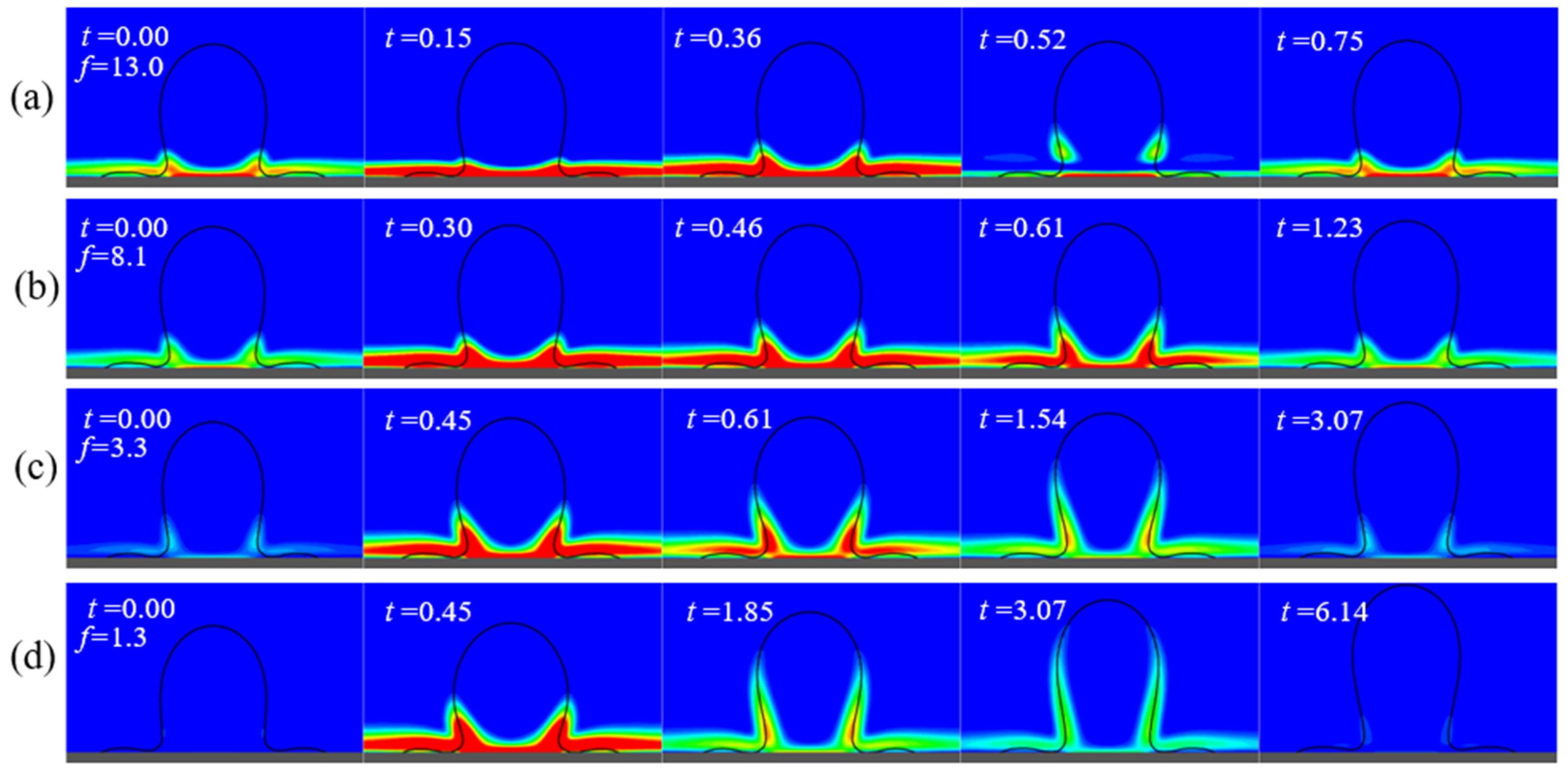
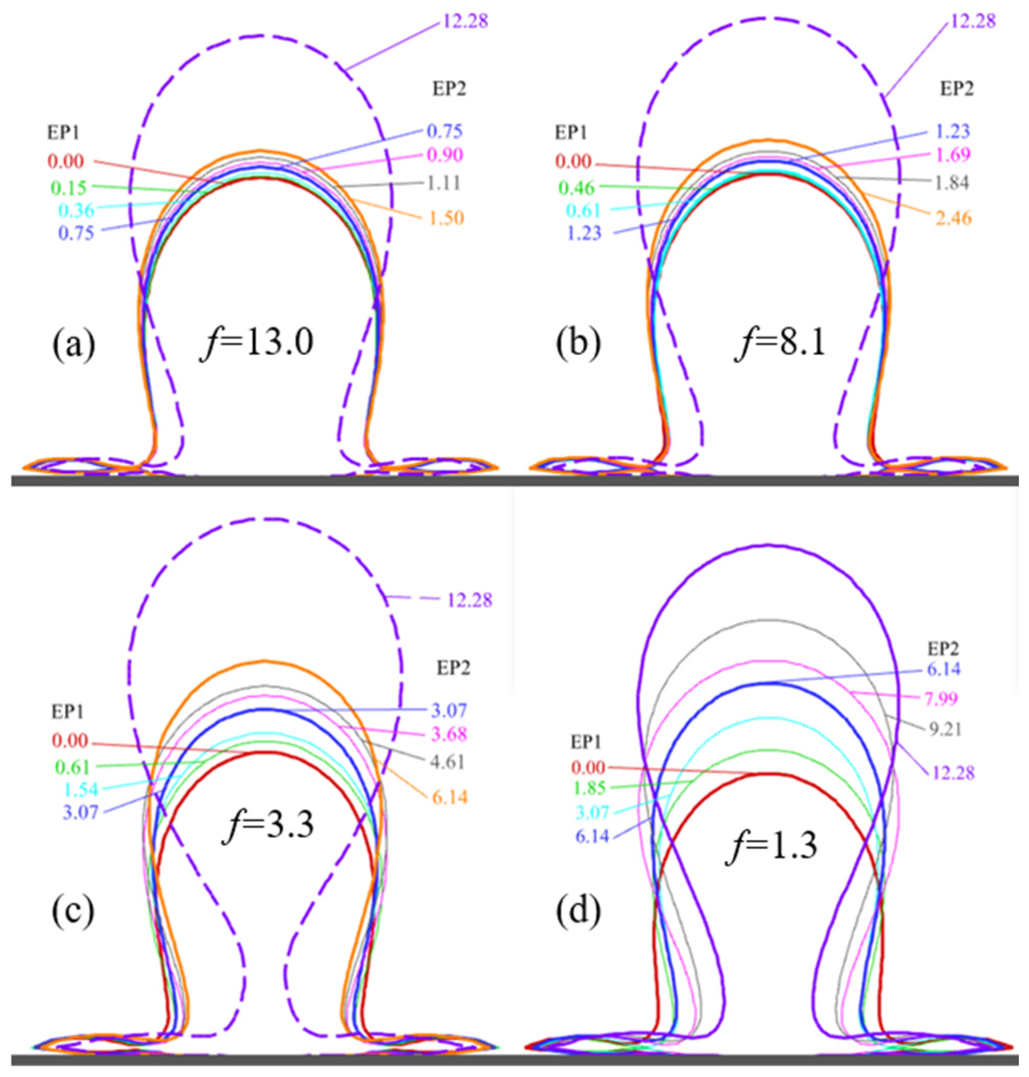
4.3. Effect of Electric Field Pulse Frequency on Bubble Behavior

To investigate the effects of pulsed electric field frequency on bubble dynamic behavior, a set of representative frequencies of pulsed electric fields were selected for conducting boiling heat transfer simulations. Figure 10 illustrates the trends of the bubble detachment period T* and detachment diameter D* as the pulse frequency f of the electric field varied from 1.3, 1.6, 1.9, 3.3, 4.5, 6.6, 8.1, 9.9, 11.9 to 13.0. From the figure, it can be seen that as f increased, both T* and D* first decreased and then increased, reaching their minimum values at f = 3.3. When f exceeded 9.9, T* and D* reached their maximum values and then stabilized. Therefore, in a pulsed electric field, the bubble detachment period and detachment diameter exhibited a nonlinear relationship with the electric field pulse frequency, and there existed an optimal pulse frequency that minimized both the detachment period and detachment diameter of the bubble.

To explain this phenomenon, the electric field forces acting on bubbles of the same size in electric field with pulse frequencies f of 13.0, 8.1, 3.3, and 1.3 were analyzed, as shown in Figure 11. For ease of discussion, the moment when the bubbles were of equal size under these four frequencies was defined as the initial zero point of the cycle. For f = 13.0, as shown in Figure 11a, a pulsed potential of V₀ = 6 was input to the lower electrode plate during the period from t = 0.00 to 0.36. As the electric field gradually diffused upward from the wall, the bottom of the bubble experienced a local electric field force that increased in area and decreased in value. Due to the high frequency, the potential of the lower electrode plate began to drop to zero at t = 0.52, causing a sudden decrease in the electric field force at the bubble’s root. Similar changes are also observed for f = 8.1, but with a slightly increased influence range of the electric field on the bubble’s root due to the lower frequency, and a correspondingly larger range of transmission toward the upper part of the bubble. However, in general, when the pulse frequency is high, due to the high-frequency transition of the electric field, the electric field force has not yet diffused to the middle of the bubble when the electric field begins to change, causing the electric field force to suddenly disappear. Therefore, under the influence of a high-frequency pulsed electric field, the electric field force only acts on the root of the bubble, with a small influence range and a short duration of pushing effect, resulting in an increase in the bubble’s detachment period and detachment diameter.

For f = 3.3, before t = 0.45, the bubble’s root had already been subjected to a large electric field force, which then gradually expanded upward, increasing its influence range. During the process from t = 0.61 to 1.54, the electric field force extended to the middle of the bubble and weakened somewhat. At this frequency, the action range of the electric field force was predominantly concentrated at the bubble’s root and the lower “V”-shaped area was connected to the root. In these two areas, the electric field force was the strongest and relatively concentrated, and the resultant force of the electric field force contributed most to the necking of the bubble’s root. Additionally, the electric field force in the “V”-shaped area also exerted a significant upward force on the bubble, enlarging its aspect ratio. Therefore, at f = 3.3, the bubble’s detachment period and detachment diameter were minimized. As the frequency further decreased to f = 1.3, as shown in Figure 11d, during the stage of t = 0.00 to 1.85, the distribution of electric field force at the bubble phase boundary was similar to that when f = 3.3. However, due to the longer period, the electric field force at the bottom had sufficient time to expand upward. At t = 1.85 to 3.07, the electric field force spread to the middle and upper parts of the bubble. Although its influence range expanded, the electric field force at the gas–liquid interface significantly decreased as a consequence of its uniform distribution within that range. The electric field force that diffused to the middle of the bubble only slightly increased the bubble’s height without causing a noticeable necking of the bubble. Therefore, at low frequencies, the detachment frequency and detachment diameter of the bubble were larger.

To further validate the enhancement effect of pulsed electric fields, Figure 12 illustrates the morphological changes of bubbles of the same size within the same duration under pulsed electric fields with frequencies of 13.0, 8.1, 3.3, and 1.3, benchmarked against two cycles of pulsed duration at f = 1.3, i.e., t = 12.28. The solid lines in the figure denote the contour changes of the bubbles over two pulsed cycles, and the purple dashed line indicates the final shape of the bubble at t = 12.28. From Figure 12a–c, the results indicate that, after two cycles of pulsed electric field application, as the pulse frequency decreased, the effect of the pulsed electric field intensified, leading to an increase in bubble height, aspect ratio, and necking speed at the bottom of the bubble. After multiple cycles of electric field exposure, when t = 12.28, the pulsed electric field at f = 3.3 exhibited the strongest effect, resulting in the largest increase in bubble aspect ratio and the fastest necking speed. From Figure 12c,d, it is evident that, at t = 6.14, the electric field at f = 1.3 acted for a longer duration, causing the bubble to grow faster. However, due to the more effective pulsed electric field at f = 3.3, after multiple cycles of pulsed electric field application, i.e., at t = 12.28, the bubble attained a higher height and faster necking speed. Therefore, the pulsed electric field at f = 3.3 demonstrates the optimal effect, with the fastest bubble necking speed and the most significant increase in aspect ratio in this.

From the above analysis, it is evident that the neck and lower “V”-shaped region of the bubble were the optimal influence zones for the electric field force to accelerate bubble necking and growth. The more concentrated the electric field force in this region and the longer it acted, the easier it was for the bubble to undergo necking, and the more significant the increase in the bubble’s aspect ratio, resulting in smaller detachment periods and detachment diameters.

5. Conclusions

In this paper, based on the two-dimensional pseudopotential LB method, the pseudopotential two-phase flow model and the ideal dielectric model were coupled to investigate the bubble dynamics behavior during pool boiling heat transfer in different electric field. The following conclusions were drawn:

(1)

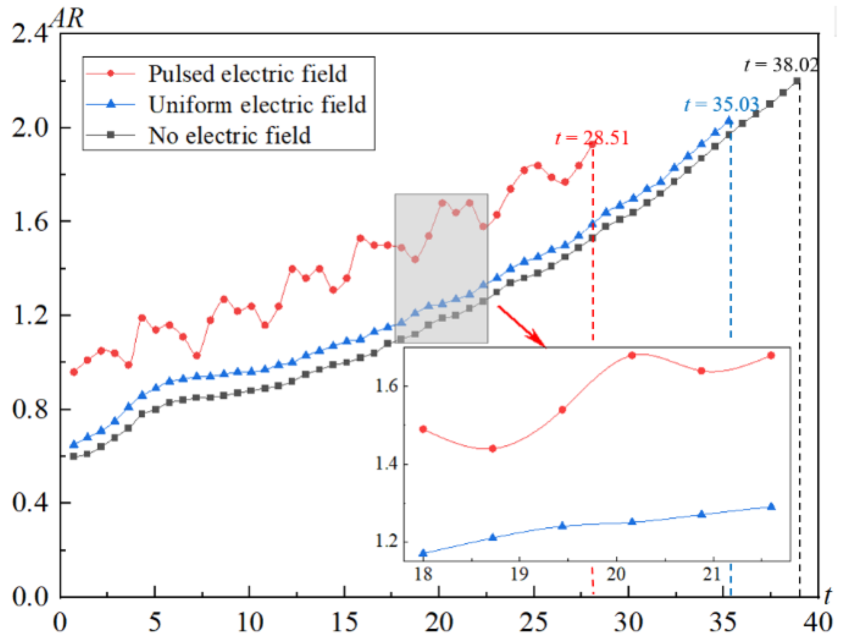
Compared with uniform electric fields and the absence of an electric field, bubbles in pulsed electric field exhibit the most pronounced morphological changes, the fastest detachment speeds, and the highest local heat flux densities at the wall surface. The aspect ratio of bubbles in a pulsed electric field is also the largest and shows a trend of oscillating increase;

(2)

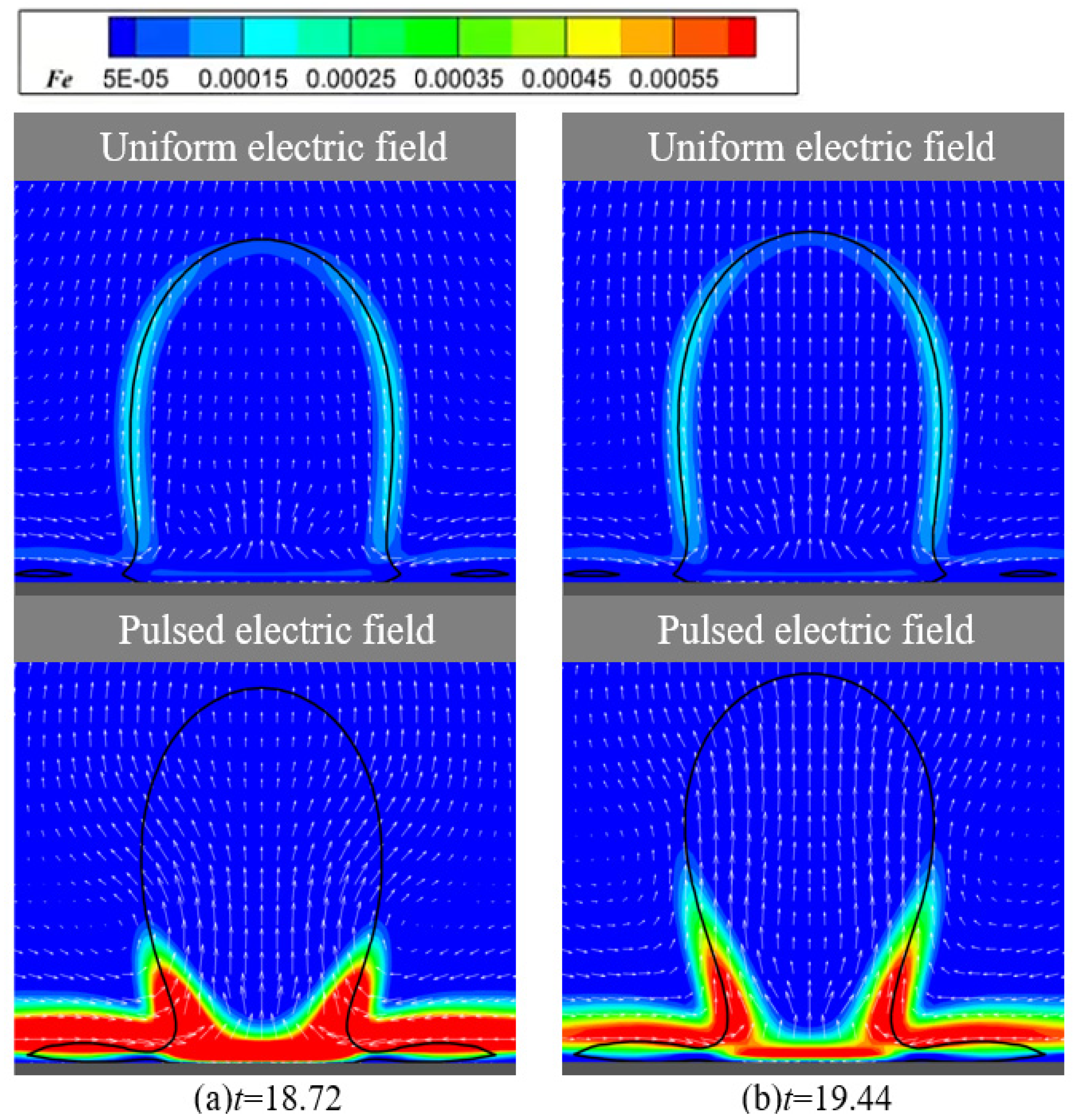
Pulsed electric fields generate abrupt changes in electric field force at the beginning and end of the peak segments of the pulse cycle. The phase boundary at the bubble base contracts subject to the electric field force, causing the internal gas to be compressed and accelerated upwards, resulting in an elongated bubble shape. In contrast, bubbles under a uniform electric field experience uniform and relatively small force changes, leading to slower internal gas flow speeds;

(3)

The detachment period and detachment diameter of bubbles first decrease and then increase as the pulse frequency increases. There exists an optimal frequency that minimizes the detachment period and detachment diameter of bubbles, resulting in the best wall heat transfer enhancement effect. The root of the bubble and the “V”-shaped region connected to the bottom of the bubble are effective areas for electric field-enhanced boiling heat transfer. The alternating action of electric field force in this region promotes early necking and detachment of the bubble, thereby enhancing boiling heat transfer.

References

1. Hong, S.; Jiang, S.; Hu, Y.; Dang, C.; Wang, S. Visualization investigation of the effects of nanocavity structure on pool boiling enhancement. Int. J. Heat Mass Transf. 2019, 136, 235–245. [Google Scholar] [CrossRef]
2. Ma, X.; Cheng, P. Dry spot dynamics and wet area fractions in pool boiling on micro-pillar and micro-cavity hydrophilic heaters: A 3D lattice Boltzmann phase-change study. Int. J. Heat Mass Transf. 2019, 141, 407–418. [Google Scholar] [CrossRef]
3. Baffigi, F.; Bartoli, C. Influence of the ultrasounds on the heat transfer in single phase free convection and in saturated pool boiling. Exp. Therm. Fluid Sci. 2012, 36, 12–21. [Google Scholar] [CrossRef]
4. Tang, J.; Xie, G.; Bao, J.; Mo, Z.; Liu, H.; Du, M. Experimental study of sound emission in subcooled pool boiling on a small heating surface. Chem. Eng. Sci. 2018, 188, 179–191. [Google Scholar] [CrossRef]
5. Luo, C.; Tagawa, T. Effect of heating wires with electric potential on pool-boiling heat transfer under an electric field. Appl. Therm. Eng. 2024, 240, 122327. [Google Scholar] [CrossRef]
6. Feng, Y.; Li, H.; Guo, K.; Lei, X.; Zhao, J. Numerical study on saturated pool boiling heat transfer in presence of a uniform electric field using lattice Boltzmann method. Int. J. Heat Mass Transf. 2019, 135, 885–896. [Google Scholar] [CrossRef]
7. Chen, Y.; Guo, J.; Liu, X.; He, D. Experiment and predicted model study of resuspended nanofluid pool boiling heat transfer under electric field. Int. Commun. Heat Mass Transf. 2022, 131, 105847. [Google Scholar] [CrossRef]
8. Madadnia, J.; Koosha, H. Electrohydrodynamic effects on characteristic of isolated bubbles in the nucleate pool boiling regime. Exp. Therm. Fluid Sci. 2003, 27, 145–150. [Google Scholar] [CrossRef]
9. Ahmad, S.; Karayiannis, T.; Kenning, D.; Luke, A. Compound effect of EHD and surface roughness in pool boiling and CHF with R-123. Appl. Therm. Eng. 2011, 31, 1994–2003. [Google Scholar] [CrossRef]
10. Chang, H.; Liu, B.; Li, Q.; Yang, X.; Zhou, P. Effects of electric field on pool boiling heat transfer over composite microstructured surfaces with microcavities on micro-pin-fins. Int. J. Heat Mass Transf. 2023, 205, 123893. [Google Scholar] [CrossRef]
11. Hristov, Y.; Zhao, D.; Kenning, D.B.R.; Sefiane, K.; Karayiannis, T.G. A study of nucleate boiling and critical heat flux with EHD enhancement. Heat Mass Transf. 2007, 45, 999–1017. [Google Scholar] [CrossRef]
12. Chen, Y.; Guo, J.; Liu, X.; Li, J.; He, D. Experiment and prediction model study on pool boiling heat transfer of water in the electric field with periodically changing direction. Int. J. Multiph. Flow 2022, 150, 104027. [Google Scholar] [CrossRef]
13. Li, X.; Chan, W.; Liang, S.; Chang, F.; Feng, Y.; Li, H. Numerical investigation on pool boiling heat transfer with trapezoidal/inverted trapezoidal micro-pillars using LBM. Int. J. Therm. Sci. 2024, 198, 108869. [Google Scholar] [CrossRef]
14. Huang, Q.; Zhou, J.; Huai, X.; Zhou, F. Studying the effect of geometry of micro-cavity on pool boiling by LBM. J. Phys. Conf. Ser. 2023, 2441, 012016. [Google Scholar] [CrossRef]
15. Shan, X.; Chen, H. Lattice Boltzmann model for simulating flows with multiple phases and components. Phys. Rev. E 1993, 47, 1815–1819. [Google Scholar] [CrossRef] [PubMed]
16. Gong, S.; Cheng, P. Numerical investigation of droplet motion and coalescence by an improved lattice Boltzmann model for phase transitions and multiphase flows. Comput. Fluids 2012, 53, 93–104. [Google Scholar] [CrossRef]
17. Cao, H.; An, Q.; Zuo, Q.; Liu, H.; Zhang, Z.; Zhao, X.; Wang, P. A New LB Model for Solid-liquid Conjugate Boiling Heat Transfer. J. Zhengzhou Univ. (Eng. Sci.) 2023, 44, 75–81. [Google Scholar]
18. Zhang, S.; Lou, Q. A mesoscopic numerical method for enhanced pool boiling heat transfer on conical surfaces under action of electric field. J. Phys. 2024, 73, 226–238. [Google Scholar] [CrossRef]
19. Li, W.; Li, Q.; Chang, H.; Yu, Y.; Tang, S. Electric field enhancement of pool boiling of dielectric fluids on pillar-structured surfaces: A lattice Boltzmann study. Phys. Fluids 2022, 34, 123327. [Google Scholar] [CrossRef]
Figure 1. Schematic diagram of computing domain (a): Schematic diagram of the calculation model, (b): Schematic diagram of bubble aspect ratio, (c): Schematic diagram of pulsed potential).
Energies 18 02540 g001
Figure 2. Model validation against Young–Laplace law.
Energies 18 02540 g002
Figure 3. Electric field model verification contour.
Energies 18 02540 g003
Figure 4. Electric field model validation ((a): x direction, (b): y direction).
Energies 18 02540 g004
Figure 5. Effect of electric field type on bubble behavior ((a): pulsed electric field, (b): uniform electric field, (c): no electric field).
Energies 18 02540 g005
Figure 6. Variation in the length–diameter ratio of bubbles under different electric field types.
Energies 18 02540 g006
Figure 7. Wall heat flux in different electric field.
Energies 18 02540 g007
Figure 8. Change in the electric field force around the bubble in response to the electric field strength in a single pulse period ((a): uniform electric field, (b): pulsed electric field).
Energies 18 02540 g008
Figure 9. The flow field varies with the electric field force.
Energies 18 02540 g009
Figure 10. Variation in bubble detachment parameters with pulse frequency (f) (a): bubble detachment period (T*), (b): bubble detachment diameter (D*)).
Energies 18 02540 g010
Figure 11. The variation in the distribution of the electric field force around the bubble in a single cycle ((a): f = 13.0, (b): f = 8.1, (c): f = 3.3, (d): f = 1.3).
Energies 18 02540 g011
Figure 12. Comparison of the effects of electric field forces over the same length of time.
Energies 18 02540 g012