Multi-Objective Optimization of Energy Storage Station Configuration in Power Grids Considering the Flexibility of Thermal Load Control

Abstract

Given that traditional grid energy storage planning neglects the impact of power supply demand on the effectiveness of storage deployment, the resulting system suffers from limited operational economic performance and restricted renewable energy integration capability. In response to this challenge, this paper presents a multi-objective optimization approach for configuring a distribution network energy storage station (ESS) by incorporating the flexibility of temperature-controlled loads. This approach aims to enhance the efficiency of energy storage utilization, facilitate the local consumption of renewable energy (RE), and achieve mutually beneficial outcomes for both energy providers and consumers. Firstly, a controllable load model for the distribution network was developed, incorporating power balance constraints and the flexibility of temperature-controlled loads. Additionally, an ESS model was formulated, taking into account economic considerations and other influencing factors to ensure optimal deployment and operation. Secondly, this paper introduces a multi-objective optimization strategy for a distribution network ESS, targeting the minimization of both the microgrid operating costs and energy storage allocation costs. The proposed model was solved using the POA-GWO-CSO optimization algorithm to achieve the optimal energy storage deployment and cost efficiency. Finally, the effectiveness of the proposed model was verified through case analysis. The results demonstrate that the proposed grid energy storage optimization configuration model not only satisfies the requirements of both parties, but also enhances the overall system economic performance.

1. Introduction

Against the backdrop of the deepening global energy transition and the increasing challenges of climate change, improving power grid adaptability and reliability has become a focal point in the field of academic research and strategic policy formulation. Nowadays, the continuous incorporation of RE, especially distributed wind as well as photovoltaic systems, which account for an increasing share of the power system, has created unprecedented challenges to the overall power system [1]. These challenges primarily stem from the variability and unpredictability of RE. On the one hand, the variability of RE prevents the power supply from maintaining a stable and continuous state, leading to fluctuating power output that disrupts the smooth operation of the power system [2]. On the other hand, its uncertainty complicates grid scheduling, making it challenging to accurately plan and optimize the power distribution and transmission. In addressing these challenges [3], efficient energy storage technology has become key, playing a buffering and regulatory role in stabilizing RE output and ensuring the normal operation of the power system and the orderly development of grid scheduling [4]. The construction phase of energy storage equipment requires the purchase of expensive core components, the installation and commissioning processes are complex, and in the subsequent operation process, maintenance and other aspects of the high cost, ultimately lead to its poor economic efficiency, so the return on investment cycle is prolonged. These factors not only discourage investor enthusiasm, but also hinder the overall development of the energy storage industry. Therefore, it is very important to strengthen the research on the optimal allocation of ESSs in the power grid [5].

Significant research efforts have been devoted to the optimal energy storage configuration by numerous scholars. Reference [6] examined the implications of the high penetration of RE on the power grid, which reduces the system’s rotational inertia, and adopted an optimized energy storage configuration method to enhance the system frequency stability. Reference [7] introduced an approach to energy storage configuration on the wind farm side to mitigate output fluctuations, ensuring that they remained within the permissible scheduling range. In [8], the authors considered the wind and solar complementary characteristics and realized the optimized allocation of wind farm and photovoltaic power station energy storage sharing through planning. Reference [9] integrated the construction and whole life cycle operation and maintenance costs of ESSs into the capacity optimization model. Their results indicated that investment costs play a crucial role among the various influencing factors and significantly impact the investment returns of energy storage facilities. Nevertheless, the aforementioned research has overlooked the substantial flexibility potential of the load side in microgrid systems, the full exploitation of which could significantly lower the energy storage configuration costs.

Simultaneously, fully exploiting the flexibility of temperature-controlled loads can significantly enhance the operational efficiency of the power grid. Air conditioning energy consumption accounts for more than 50% of the total building energy use. By fully leveraging the temperature-controlled load flexibility [10], the energy use flexibility of air conditioning systems can be effectively enhanced. In Reference [11], office buildings with integrated air conditioning systems were further incorporated into a hybrid energy microgrid, where the virtual energy storage effect of air conditioning loads was leveraged to achieve a reduction in the operating costs. In [12], the study applied temperature-controlled load flexibility to the cogeneration system, greatly enhancing the cogeneration system’s operational flexibility. Reference [13] established a combined heat and power system model based on temperature-controlled load flexibility, which fully considered the interaction and synergistic relationship between the two forms of energy, electricity and heat, and realized the best economy. However, the existing studies exhibited significant limitations in the coordinated optimization of energy storage stations and power grids. Most notably, the temperature-controlled load model of the load side has not been systematically incorporated into system modeling and optimization processes, thereby neglecting the substantial potential for flexible regulation. In addition, the role of energy storage stations in reducing the grid operation costs and the exploitation of temperature-controlled load flexibility have not been sufficiently addressed, resulting in the failure to achieve coordinated minimization of the microgrid and energy storage station operation costs.

Meanwhile, in terms of multi-objective optimal configuration algorithms for grid energy storage power stations, a high-quality algorithm with fast convergence speed, good parameter adaptability, and high engineering practicability is crucial. In [14], in light of the aging and wear and tear of photovoltaic power station equipment prone to fire, the authors proposed a fire control system based on the multi-objective particle swarm algorithm and Internet of Things technology, which effectively improved the fire control efficiency and ensured the safe and stable operation of the ESS. Reference [15], in light of the complexity of grid reactive power optimization, proposed improving the genetic simulated annealing algorithm so that the algorithm could reduce the loss and accelerate the convergence. However, the multi-objective particle swarm optimization algorithm tended to converge to the local optima, and its performance was highly dependent on parameter selection. At the same time, the improved genetic simulated annealing algorithm was computationally complex when dealing with large-scale power grids, and the parameter settings depended on empirical debugging, which will affect the results if the parameters are not appropriate. Reference [16] proposed an optimization method based on an improved pelican optimization algorithm for the optimal economic operation of the energy management strategy in multi-terminal AC/DC flexible interconnection systems. This method enabled optimal scheduling of the system, exhibiting strong global search capabilities and effectively avoiding entrapment in the local optima. However, it suffered from a relatively long convergence time and low computational efficiency.

Therefore, this paper proposes a multi-objective optimization method based on the POA-GWO-CSO, which simultaneously considers both the grid operation cost and the energy storage station configuration cost. An optimization model was established with the objectives of minimizing the grid operation costs and minimizing the energy storage station configuration costs. The method introduces the leader strategy from the grey wolf optimization algorithm (GWO) and the crisscross optimization algorithm (CSO) to enhance the pelican position update mechanism in the original pelican optimization algorithm (POA). Finally, the improved POA-GWO algorithm was applied to solve the multi-objective optimization model for the grid and energy storage system, demonstrating that the enhanced algorithm achieved higher computational efficiency.

In summary, the current research still has two main limitations. First, traditional energy storage configuration approaches often overlook the impact of demand-side load flexibility, resulting in limited potential for economic performance improvement. Second, existing optimization algorithms still require further enhancement in terms of computational efficiency and global search capability. To address these issues, this paper proposed a multi-objective optimization method for configuring ESSs in power grids by incorporating the flexibility of temperature-controlled loads. The main contributions of this study are threefold. First, a controllable load modeling framework was developed that simultaneously accounted for the power balance constraints and the dynamic response characteristics of the temperature-controlled loads, thereby overcoming the limitations of existing models that focus predominantly on the supply side. Second, a multi-objective optimization model was formulated to minimize both the operating costs of the grid and the configuration costs of the ESS, and a hybrid POA-GWO-CSO algorithm was employed to ensure rapid convergence and high-quality solutions. Third, the flexibility potential of temperature-controlled loads was fully exploited by introducing a comfort temperature range for users, which, while maintaining indoor thermal comfort, enabled the simultaneous improvement in the profitability of energy storage systems and the consumption rate of renewable energy. The remainder of this paper is organized as follows. Section 2 introduces the overall operational framework of the grid-integrated energy storage station; Section 3 establishes the mathematical models for the power grid, the energy storage system, and temperature-controlled loads; Section 4 presents the multi-objective optimization strategy focusing on the ESS configuration and grid operating costs; Section 5 provides a detailed explanation of the POA-GWO-CSO hybrid optimization algorithm and its implementation process; Section 6 analyzes the system operational characteristics and economic performance under different configuration scenarios through case studies to validate the effectiveness of the proposed method; and Section 7 concludes the paper by summarizing the main findings and outlining future research directions.

2. Operational Framework for ESS in the Power Grid

The framework is shown in Figure 1. In this framework, it includes the ESS, numerous controllable building loads, and the distribution system. The controllable building loads can be powered by photovoltaics, wind power, energy storage stations, and the grid. Their energy primarily originates from conventional electrical loads and air-conditioning loads [17,18]. The ESS features a control center that manages scheduling instructions according to the charging and discharging requirements of controllable building loads in each time period. When a building load requires charging, the control center utilizes the energy storage system to retain surplus electricity and adjusts the charging or discharging based on the load demands [19]. The energy storage power station control center determines the appropriate capacity and peak charging and discharging power by analyzing the cyclic behavior of all controllable building loads. Furthermore, it administers user payments and pricing in alignment with time-of-use electricity tariffs. This mechanism optimizes energy storage utilization, supports the local integration of renewable energy, and ensures mutually beneficial outcomes for all stakeholders [20,21].

3. Power Grid and ESS Model

3.1. Power Grid Model

The building load model considered in this paper was the temperature controlled load model, as shown in Equations (1)–(3):

$$T_{\min }\le T_{\mathrm{t}}\le T_{\max }$$

(1)

$$0\le P_t\le P^{\max }$$

(2)

$$C\left(T_{t+1}-T_t\right)=\Delta t({\displaystyle \frac{T_{out,t}-T_t}{R_{wa}}}+{\displaystyle \frac{T_{out,t}-T_t}{R_w}}+C_{GP}\cdot P_t+M_t^{rad}\cdot k\cdot F_w+Q_{in})$$

(3)

where $T_{\min }$ and $T_{\max }$ indicate the minimum and maximum limits of the comfort temperature, respectively; $T_{\mathrm{t}}$ indicates the indoor temperature; $C$ indicates the heat capacity of the wall; $T_{out,t}$ indicates the outdoor temperature; $C_{GP}$ indicates the EER of the air conditioning; $P^{\max }$ indicates the rated power of the air conditioning; $R_{wa}$, $R_w$ indicate the thermal resistance of the wall and the window, respectively; k indicates the transmission rate of the window; $M_t^{rad}$ indicates the intensity of the sunlight; $Q_{in}$ indicates the heating power of the internal heat source; and $F_w$ indicates the area of the external window.

The operating costs of the grid include the power purchase costs, generation costs, network loss costs, and load costs as follows:

• Cost of purchasing electricity $C_{\mathrm{grid}}$

  $$C_{\mathrm{grid}}={\displaystyle \sum _{t=1}^{24}{c}_{\mathrm{buy}}^t{P}_{\mathrm{grid}}^t\Delta t}$$

  (4)

  where $c_{\mathrm{buy}}^t$ is the electricity purchase price in period t; $P_{\mathrm{grid}}^t$ is the power transfer between the grid and the system in period t; $\Delta t$ is the length of the scheduling interval.
• Power generation costs

  $$C_{\mathrm{DG}}={\displaystyle \sum _{t=1}^{24}{\displaystyle \sum _{i\in {\mathrm{\Omega }}_{\mathrm{MG}}}(c_{\mathrm{MG}}^{\mathrm{fuel}}\frac{P_{\mathrm{MG},i}^t}{{\eta }_i}+c_{\mathrm{MG}}^{\mathrm{oper}}{P}_{\mathrm{MG},i}^t)\Delta t}}$$

  (5)

  where ${\mathrm{\Omega }}_{MG}$ is the set of micro-gas turbine units for any micro-gas turbine i in the set ${\mathrm{\Omega }}_{MG}$; $c_{\mathrm{MG}}^{\mathrm{fuel}}$ and $c_{\mathrm{MG}}^{\mathrm{oper}}$ are the unit fuel operation and maintenance costs, respectively; $P_{\mathrm{MG},i}^t$ is the power generated; ${\eta }_i$ is the conversion efficiency.
• Network loss costs

  $$C_{\mathrm{loss}}={\displaystyle \sum _{t=1}^{24}{c}_{\mathrm{buy}}^t}{\displaystyle \sum _{j=1}^{N_{\mathrm{node}}}{u}_j^t}{\displaystyle \sum _{k\in {\mathsf{\Omega }}_j^{\mathrm{L}}}{u}_k^t{G}_{jk}\cos {\delta }_{jk}^t\Delta t}$$

  (6)

  where $N_{\mathrm{node}}$ represents the total number of nodes; $u_j^t$, $u_k^t$ represent the voltage amplitude of nodes j and k at time t, respectively; $G_{jk}$ represents the conductance between nodes j and k; ${\delta }_{jk}^t$ and represents the phase angle difference of the voltages of nodes j and k.
• Load cost

  $$C_{\mathrm{LO}}={\displaystyle \sum _{t=1}^{24}{c}_{\mathrm{buy}}^t}(P_t+P_{load})$$

  (7)

  where $P_{load}$ is the conventional electrical load.

3.2. ESS Model

Among the many types of equipment that can be selected for the ESS, battery energy storage technology has a high degree of maturity, has been realized in many areas of large-scale application, and is one of the most common energy storage devices in the power grid. The relationship between the remaining battery power $S_{\mathrm{SB}}\left(t\right)$ at moment t and the remaining battery power $S_{\mathrm{SB}}(t-1)$ at the moment of $t-1$ is shown in Equation (8); in the case of discharge, the relationship between the two is as shown in Equation (9).

When charging, the ESS is as follows:

$$S_{\mathrm{SB}}\left(t\right)=S_{\mathrm{SB}}(t-1)+{\eta }_{\mathrm{ch}}{P}_{\mathrm{ch}}(t)\Delta t-\lambda Q_{\mathrm{SB}}$$

(8)

When discharging, the ESS is as follows:

$$S_{\mathrm{SB}}(t)=S_{\mathrm{SB}}(t-1)-{\displaystyle \frac{P_{\mathrm{dis}}\left(t\right)}{{\eta }_{\mathrm{dis}}}}\Delta t-\lambda Q_{\mathrm{SB}}$$

(9)

where $P_{\mathrm{ch}}\left(t\right)$, ${\eta }_{\mathrm{ch}}$, $P_{\mathrm{dis}}\left(t\right)$, ${\eta }_{\mathrm{dis}}$ represent the battery’s charging and discharging power and efficiency, respectively; $\lambda$, $Q_{\mathrm{SB}}$ represent the self-discharge rate and capacity of the battery, respectively. The optimization of the ESS configuration costs specifically involves the following aspects.

• Acquisition costs

The acquisition cost of the ESS is the main component of its comprehensive configuration cost, which significantly affects the economic performance of the optimal configuration of the system. In the economic analysis of the energy storage system and the optimal configuration decision, it is not enough to only consider the acquisition cost, but there is also a need to use the whole life cycle cost model to calculate and predict the comprehensive cost of the energy storage system. The acquisition cost of the ESS is shown in Equation (10) as follows:

$$C_1={\displaystyle \sum _{i=1}^n}{\displaystyle \frac{r{(1+r)}^D}{{\left(1+r\right)}^D-1}}[Q_i{c}_i(n_i+1)]$$

(10)

where $N$ represents the ESS count; r represents the prime rate; $Q_i$ represents the configured capacity of the ith ESS; $n_i$ represents the number of replacement times of the ith ESS in the planning years.

2.

Installation costs

During the construction of the ESS, procurement and installation often involve different manufacturers and companies. Even if the procurement and installation are carried out by the same company, the installation cost needs to be calculated separately because the scale of the energy storage project is usually large [22]. Therefore, a detailed modeling analysis is needed when considering the comprehensive optimal configuration cost of the ESS, which is shown in Equation (11).

$$C_2={\displaystyle \sum _{i=1}^N{\displaystyle \sum _{j=1}^{n_i}\frac{r{\left(1+r\right)}^D}{{\left(1+r\right)}^D-1}{\left(1+r\right)}^{-d_{i}j}{\left(1-{\alpha }_i\right)}^{d_{i}j}{C}_{\mathrm{rep}}^{i,j}{N}_i}}$$

(11)

where $C_{\mathrm{rep}}^{i,j}$ represents the jth installation cost of the ith ESS; ${\alpha }_i$ represents the average annual decrease factor of the installation cost of the ith ESS.

3.

Operation and maintenance (O&M) costs

The daily operation of the ESS involves storing and releasing electricity, and costs are invested to ensure the safe and reliable operation of the system. These costs cover personnel, management, and parts replacement. Personnel costs include daily monitoring, fault diagnosis and elimination, and regular inspections by a professional operation and technical maintenance team; management costs include project management, financial management, and other management activities; and the regular inspection and replacement of parts, if necessary, are also important operation and maintenance expenses. These inputs ensure the performance and reliability of the ESS throughout its life cycle [23], and the O&M cost of the ESS during its full life cycle is shown in Equation (12):

$$C_3={\displaystyle \sum _{i=1}^N{\displaystyle \sum _{t=1}^T\left[u_{i,1}\right(t\left)\right|P_{\mathrm{SB},\mathrm{i}}\left(t\right)|k_{\mathrm{ch}}+u_{2,i}(t\left)\right|P_{\mathrm{SB},\mathrm{i}}\left(t\right)\left|k_{\mathrm{dis}}\right]}}$$

(12)

where $P_{\mathrm{SB},\mathrm{i}}\left(t\right)$ represents the charging and discharging power of the ith ESS in the t moment period; the ESS is in the discharging state when $P_{\mathrm{SB},\mathrm{i}}\left(t\right)\ge 0$, the ESS is in the charging state when $P_{\mathrm{SB},\mathrm{i}}\left(t\right)\le 0$. $k_{\mathrm{ch},\mathrm{i}}$ represents the O&M cost coefficient when charging the ith ESS; $u_{i,1}\left(t\right)$ represents the storage charging coefficient, $u_{2,i}\left(t\right)$ represents the storage discharging coefficient when charging the storage, $u_{i,1}\left(t\right)=1$ and $u_{2,i}\left(t\right)=0$, when discharging the storage, $u_{i,1}\left(t\right)=0$ and $u_{2,i}\left(t\right)=1$; $k_{\mathrm{dis},\mathrm{i}}$ represents the O&M cost of the ith storage discharging coefficient, which is calculated as shown in Equations (13) and (14), respectively.

$$k_{\mathrm{ch},\mathrm{i}}={\displaystyle \frac{C_{\mathrm{init}}}{N\left(x\right)}}\cdot {\displaystyle \frac{c_{\mathrm{ch}}}{-P_{\mathrm{SB},\mathrm{i}}\left(t\right)S_{\mathrm{SB},\mathrm{start}}}}\cdot {\displaystyle \frac{S_{\mathrm{SB}}^{\max }}{S_{\mathrm{SB},\mathrm{end}}}}$$

(13)

$$k_{\mathrm{dis},\mathrm{i}}={\displaystyle \frac{C_{\mathrm{init}}}{N\left(x\right)}}\cdot {\displaystyle \frac{c_{\mathrm{dis}}}{P_{\mathrm{SB},\mathrm{i}}\left(t\right)S_{\mathrm{SB},\mathrm{end}}}}\cdot {\displaystyle \frac{S_{\mathrm{SB},\mathrm{start}}}{S_{\mathrm{SB}}^{\max }}}$$

(14)

where $N\left(x\right)$ represents the maximum number of cycles; $C_{\mathrm{init}}$ represents the initial fixed investment cost of the ESS; $S_{\mathrm{SB},\mathrm{start}}$, $S_{\mathrm{SB},\mathrm{end}}$ are the initial and final charge state of the ESS, respectively; $S_{\mathrm{SB}}^{\max }$ represents the maximum residual power; $c_{\mathrm{ch}}$ and $c_{\mathrm{dis}}$ are the charging and discharging impact factors, respectively.

4.

Equipment residual value recovery

When the ESS reaches the end of its service life, the residual value of its equipment can be obtained through recycling, reuse, or transfer, etc. Including this part of the residual value in the calculation of the comprehensive configuration cost can effectively reduce the overall investment cost of the project, improve the return on investment, enhance the economic benefits of the whole project, and reduce the waste of resources and promote the development of a circular economy. Therefore, when carrying out the economic assessment and configuration decision-making work of the ESS, it is crucial to fully consider the factor of the equipment residual value recovery to optimize the economy and sustainability of the project [24], which is calculated as shown in Equation (15):

$$C_4={\displaystyle \sum _{i=1}^N{\displaystyle \sum _{j=0}^{n_i}\frac{r{(1+r)}^D}{{\left(1+r\right)}^D-1}{\left(1+r\right)}^{-d_{i}j}{C}_{4,i}{N}_i}}$$

(15)

where $C_{4,i}$ represents the residual value of the ith ESS. In Equation (16),

$$C_{4,i}=k_{\nu al}{Q}_i$$

(16)

where $k_{\nu al}$ represents the residual value coefficient of the energy storage station.

3.3. Constraints

• Grid node voltage and line current constraints

  $$\left\{\begin{array}{c}{U}_{\min }⩽U_{i,\left(t\right)}⩽U_{\max }\\ \left|I_{ij,\left(t\right)}\right|⩽I_{ij,\max }\end{array}\right.$$

  (17)

  where $U_{\max }$, $U_{\min }$ are the upper and lower limit values of the node voltage, respectively; $I_{ij,\max }$ indicates the maximum current carrying capacity of the line between node i and node j.
• Power balance constraints

  $$\sum (P^{\mathrm{ES}}+P^{\mathrm{ESS}}+P^{\mathrm{PV}}+P^{\mathrm{WT}})=\sum (P^{\mathrm{load}}+P^{\mathrm{loss}})$$

  (18)

  where $P^{\mathrm{ES}}$, $P^{\mathrm{ESS}}$, $P^{\mathrm{PV}}$, $P^{\mathrm{WT}}$ are the grid power, energy storage system, photovoltaic, wind power grid power, respectively; $P^{\mathrm{load}}$, $P^{\mathrm{loss}}$ are the system load power and system active loss, respectively.
• Grid tributary current constraints

  $$v_{m,t}-v_{n,t}=2(r_{mn}{P}_{mn,t}+x_{mn}{Q}_{mn,t})-(r_{mn}^2+x_{mn}^2)i_{mn,t}$$

  (19)

  $$i_{mn,t}{v}_{m,t}=P_{mn,t}^2+Q_{mn,t}^2$$

  (20)

  $$P_{\mathrm{in},n,t}=\sum _{l:n\to l}{P}_{nl,t}-(P_{mn,t}-i_{nm,t}{r}_{nm})$$

  (21)

  $$Q_{\mathrm{in},n,t}=\sum _{l:n\to l}{Q}_{nl,t}-(Q_{mn,t}-i_{mn,t}{x}_{mn})$$

  (22)

  where $v_{m,t}$ and $v_{n,t}$ are the squares of the voltage magnitudes at nodes m and n, respectively; $i_{mn,t}$ is the square of the current magnitude of line mn; $r_{nm}$ and $x_{mn}$ are the resistance and reactance of line mn, respectively; l is a sub-node of node n. $P_{mn,t}$ and $P_{\mathrm{in},n,t}$ denote the active power injected into the sides of nodes m and n, respectively; $Q_{mn,t}$ and $Q_{\mathrm{in},n,t}$ denote the reactive power injected into the sides of nodes m and n, respectively.
• Energy storage battery (ESB) capacity and energy multiplier constraints

  $$\left\{\begin{array}{l}{E}_{B,\min }^{\mathrm{ESS}}⩽E_B^{\mathrm{ESS}}⩽E_{B,\max }^{\mathrm{ESS}}\\ E_B^{\mathrm{ESS}}=\beta \cdot P_B^{\mathrm{ESS}}\end{array}\right.$$

  (23)

  where β is the energy multiplier of the ESB; $E_{B,\max }^{\mathrm{ESS}}$, $E_{B,\min }^{\mathrm{ESS}}$ are the upper and lower limits of the rated capacity of the ESB, respectively; $P_{B,\max }^{\mathrm{ESS}}$, $P_{B,\min }^{\mathrm{ESS}}$ are the upper and lower limits of the charging and discharging power of the ESB, respectively.
• ESB charge state constraints

  $$\left\{\begin{array}{l}\begin{array}{l}{S}_{\min }^{\mathrm{SOC}}⩽S_{\left(t\right)}^{\mathrm{SOC}}⩽S_{\max }^{\mathrm{SOC}}\\ \left|P_{B,\min }^{\mathrm{ESS}}\right|⩽\left|P_{\left(i\right)}^{\mathrm{ESS}}\right|⩽\left|P_{B,\max }^{\mathrm{ESS}}\right|\end{array}\hfill \\ S_s^{\mathrm{SOC}}=S_e^{\mathrm{SOC}}\hfill \end{array}\right.$$

  (24)

  where $S_{\max }^{\mathrm{SOC}}$, $S_{\min }^{\mathrm{SOC}}$,$P_{B,\max }^{\mathrm{ESS}}$, $P_{B,\min }^{\mathrm{ESS}}$ represent the depth of charge and discharge and the upper and lower power limits of the ESB, respectively.;$S_s^{\mathrm{SOC}}$, $S_e^{\mathrm{SOC}}$ are the charging state of the ESB at the beginning and the end of the operating cycle, respectively.
• Voltage offset constraints

  $$U_{\mathrm{lev}}={\displaystyle \frac{1}{T}}{\displaystyle \sum _{i=1}^n\left[{\displaystyle \sum _{i=1}^N{\left(\frac{U_{i,\left(t\right)}-U_i^{\ast }}{\Delta U_{i,\max }}\right)}^2}\right]}$$

  (25)

  $$0\le U_{\mathrm{lev}}\le U_{lex}^{\max }$$

  (26)

  where $U_{\mathrm{lev}}$ is the voltage offset during grid operation; N is the number of load nodes; T is the time period; $U_{i,\left(t\right)}$ and $U_i^{\ast }$ are the voltage of the ith node and the reference voltage at time t, respectively; $\Delta U_{i,\max }$ is the maximum permissible deviation of the voltage of the ith node; $U_{lex}^{\max }$ is the maximum permissible voltage offset during grid operation.

4. Multi-Objective Optimization Strategy for Grid Energy Storage Stations Taking into Account Temperature-Controlled Load Flexibility

The multi-objective optimal allocation method of the ESS taking into account the controllable load flexibility and grid balance aims to obtain the solution with the lowest grid operating cost and the smallest allocation cost of the ESS [25].

$$\left\{\begin{array}{l}{F}_1=\min \left\{C_{grid}+C_{loss}+C_{DG}+C_{LO}\right\}\\ F_2=\min \left\{C_1+C_2+C_3-C_4\right\}\end{array}\right.$$

(27)

The grid-side modeling of the above model is mainly based on the grid branch current model. However, the nonlinear nature of the power system makes finding the global optimal solution extremely difficult. This is because the nonconvex problem may contain multiple local optimal solutions, and the optimization algorithm may fall into these local solutions instead of finding the global optimal solution. To solve this problem, the second-order cone relaxation (SOCR) technique can be used. This method converts the original problem into a convex problem that is easier to solve by relaxing the nonconvex part of the problem. Specifically, SOCR converts the nonconvex quadratic constraints into a series of second-order cone constraints, thus obtaining a second-order cone programming (SOCP) model. SOCP is a special kind of convex optimization problem, whose standard form is as follows:

$$F_{\mathrm{socp}}=\min \left\{c^{T}x|Ax=b,x\in H\right\}$$

(28)

where x is a vector of decision variables; b, c, and $A$ are vectors of constants; $c^{T}x$ is a linear function of x; $H$ is as follows:

Second-order cone:

$$H=\left\{x_i\in R_N|y^2\ge \sum _{i=1}^N{x}_i^2,y\ge 0\}\right\}$$

(29)

Rotate the second-order cone:

$$H=\left\{x_i\in R_N|yz\ge \sum _{i=1}^N{x}_i^2,y,z\ge 0\}\right\}$$

(30)

The SOCP model has been widely recognized and applied in the field of power system optimization due to its balance between computational efficiency and solution accuracy. It transforms complex problems containing nonconvex nonlinear constraints into convex optimization problems through mathematical transformations, which substantially improve the solution efficiency and solution quality. Based on the SOCP model, Equation (20) can be written as:

$${‖ {\left[2P_{mn,t}\hspace{1em}2Q_{mn,t}\hspace{1em}{i}_{mn,t}-v_{m,t}\right]}^{\mathrm{T}}‖}_2\le i_{mn,t}+v_{m,t}$$

(31)

To calibrate the accuracy of the above model, the SOCR error gap needs to be further calculated with the following relaxation:

$${\Delta }_{\mathrm{diff},t}=P_{mn,t}^2+Q_{mn,t}^2-i_{mn,t}{V}_{m,t}$$

(32)

When the error gap reaches the set accuracy, the corresponding optimal solution can be considered to be equivalent to the actual optimal solution.

5. POA-GWO-CSO Algorithm

This paper employed the POA-GWO-CSO algorithm to solve the multi-objective optimal allocation problem of an energy storage station that takes into account controllable load flexibility and grid balance. The algorithm combines three optimization strategies:

• Pelican optimization algorithm

This algorithm is a meta-heuristic optimization algorithm that operates by simulating the pelican’s predatory behavior in order to carry out the optimization search. The algorithm consists of a move-to-prey phase and a skimming-over-the-water phase, in which the position of the pelican is continuously updated to get closer to the optimal solution.

In the initial phase of the POA, a population of individuals with uniformly distributed random values is generated, similar to traditional optimization algorithms. Each individual corresponds to a set of variable values for the objective function. This random initialization ensures population diversity, facilitating an exploration of the solution space from various directions and thereby increasing the likelihood of identifying superior solutions.

The specific steps are as follows: the first step is population initialization. If there are n pelicans in the m-dimensional space, the position of the ith pelican is $X_i=[X_{i1},X_{i2},\dots ,X_{im}]$, and the positions of the n pelicans are

$$X=\left[\begin{array}{c}{X}_1\\ X_2\\ ⋮\\ X_n\end{array}\right]\left[\begin{array}{cccc}{x}_{11}& x_{12}& \dots & x_{1m}\\ x_{21}& x_{22}& \dots & x_{2m}\\ ⋮& ⋮& ⋮& ⋮\\ x_{n1}& x_{n2}& \dots & x_{nm}\end{array}\right]$$

(33)

The population initialization can be expressed as

$$x_{ij}=f_j+R(f_j-g_j)$$

(34)

where R is a rand number in [0,1]; f_j, g_j are the upper and lower bounds of the solution problem in dimension j, respectively.

The second phase, known as the move-to-prey stage, models the ability of the pelican group to enhance the search space exploration and identification of potential solutions through collective cooperation and information sharing upon locating prey. During this phase, each individual pelican updates its position relative to the currently best-known position, following a strategy that incorporates both randomness and directionality, thereby maintaining a balance between global exploration and convergence toward superior solutions. Its specific mathematical expression is as follows

$$x_{ij}^{p_1}=\left\{\begin{array}{l}{x}_{ij}+\delta \left(P_j-I{x}_{ij}\right),f_P\left(x_{ij}^{p_1}\right)<f\left(x_{ij}^{p_1}\right)\hfill \\ x_{ij}+\delta \left(x_{ij}-P_j\right),else\hfill \end{array}\right.$$

(35)

where $x_{ij}^{p_1}$ is the position of the ith pelican in the jth dimension after the first step; P_j is the position of the prey in the jth dimension; δ is any number in [0,1]; I is randomly 1 or 2; $f_P\left(x_{ij}^{p_1}\right)$, $f\left(x_{ij}^{p_1}\right)$ are the fitness function values of the prey and the pelican, respectively.

After the update, if the objective function value at the new position improves, the position is updated according to Equation (36). This adaptive mechanism allows the algorithm to dynamically adjust its search strategy based on changes in the objective function value, thereby concentrating the search process more effectively in the vicinity of potential optimal solutions. As a result, both the search efficiency and the quality of the obtained solutions are significantly enhanced.

$$X_i=\left\{\begin{array}{l}{X}_i^{p_1},f_i^{p_1}\left(x_{ij}^{p_1}\right)<f\left(x_{ij}^{p_1}\right)\hfill \\ X_i,else\hfill \end{array}\right.$$

(36)

where $X_i^{p_1}$ is the new position of the ith pelican in the first step; $f_i^{p_1}\left(x_{ij}^{p_1}\right)$ is the adaptation value of the ith pelican in the new position after updating in the first step.

The third step is the skimming-over-the-water phase, which balances the characteristics of the objective function and the trade-off between exploration and exploitation by simulating the pelican’s feeding behavior during skimming. In this phase, the pelican searches in the vicinity of the current solution, focusing on potential high-quality solutions, analogous to the pelican spreading its wings to lift fish toward the surface. This strategy enables the algorithm to concentrate on the surroundings of promising solutions, thereby enhancing the search efficiency and solution quality while maintaining the global exploration capabilities and strengthening the local search performance, ultimately leading to faster convergence toward the optimal solution.

$$x_{ij}^{p_2}=x_{ij}+Y(1-{\displaystyle \frac{t}{T}})\left({\displaystyle \frac{1}{Y}}\beta -1\right)x_{ij}$$

(37)

where $x_{ij}^{p_2}$ is the position of the ith pelican in the jth dimension after the second stage update; Y is a non-zero number within 0~1; ${\displaystyle \frac{t}{T}}$ is the ratio of the number of iterations; β is randomly 1 or 2.

After the second stage update, if the position leads to a better objective function value, then the position is updated to the newly discovered position

$$X_i=\left\{\begin{array}{l}{X}_i^{p_2},f_i^{p_2}\left(x_{ij}^{p_2}\right)<f\left(x_{ij}^{p_2}\right)\hfill \\ X_i,else\hfill \end{array}\right.$$

(38)

where $X_i^{p_2}$ is the new position of the ith pelican in the second step; $f_i^{p_2}\left(x_{ij}^{p_2}\right)$ is the fitness value of the ith pelican in the new position after the update in the second step.

2.

Gray wolf optimization algorithm

By introducing the wolf pack leader strategy, the behavior of α, β, and δ wolf leadership groups in the gray wolf society is simulated in order to carry out the search, which can enhance the algorithm’s global search ability and effectively avoid falling into the dilemma of local optimal solutions.

The specific steps are as follows. First, a nonlinear inertia weight factor p and a nonlinear inertia weight coefficient q are introduced to ensure that the inertia weight factor p can be dynamically adjusted according to the requirements of the current search state. This adjustment enhances the adaptability and flexibility of the algorithm, enabling it to better cope with complex search spaces. The expression for the weight value p(t) of the number of iterations at time t is as follows:

$$p(t)={\displaystyle \frac{p_{\max }-p_{\min }}{1+\exp \left[-q\left(t-\frac{T}{2}\right)\right]}}+p_{\min }$$

(39)

where p_max and p_min are the maximum/minimum weight factors, respectively.

A wolf pack is usually led by α, β, and δ wolves in the hunting process, which represent the leader, sub-leader, and third leader in the pack, respectively. These three types of wolves guide the wolf pack close to the prey through collaborative cooperation while constantly adjusting individual positions in the process to optimize the search strategy.

$$\left\{\begin{array}{l}{K}_1=I_{\alpha }-A_1\cdot \left|C_1\times I_{\alpha }(t)-I(t)\right|\\ K_2=I_{\beta }-A_2\cdot \left|C_2\times I_{\beta }(t)-I(t)\right|\\ K_3=I_{\delta }-A_3\cdot \left|C_3\times I_{\delta }(t)-I(t)\right|\end{array}\right.$$

(40)

$$K=(K_1+K_2+K_3)/3$$

(41)

where $K_1,K_2,K_3$ is the influence between the $\alpha ,\beta ,\delta$ wolf and other wolves, respectively; $A_1,A_2,A_3$ is a random number; $C_1,C_2,C_3$ is the perturbation coefficient parameter; $I_{\alpha },I_{\beta },I_{\delta }$ is the current position of the prey; $I\left(t\right)$ is the position of the individual gray wolf after t iterations.

GWO simulates the social hierarchical structure and hunting behavior of gray wolves, which not only ensures good convergence, but also maintains the population diversity and avoids premature convergence to local optimal solutions. The algorithm guides the search process through a set of dynamic update formulas, which are formulated as follows:

$$x_t^1=\left\{\begin{array}{l}{F}_t+K[(ub-lb)a_1+lb],a_2⩾0.5\hfill \\ F_t-K[(ub-lb)a_1+lb],a_2<0.5\hfill \end{array}\right.$$

(42)

where $x_t^1$, F_t are denoted as the position of the individual and food in dimension t, respectively; ub, lb are the upper and lower limits of the optimization seeking position, respectively; a₁, a₂ are random numbers.

Based on the GWO strategy, Equation (35) can be written as

$$x_{ij}^{p_1}=\left\{\begin{array}{l}w{x}_{ij}+{\displaystyle \frac{x_t^1-F_t}{(1+a_2)\cdot ub}}(P_j-I{x}_{ij}),F_P<F \mathrm{and} a_2⩾0.5\\ w{x}_{ij}+{\displaystyle \frac{F_t-x_t^1}{(1+a_2)\cdot ub}}(x_{ij}-P_j),else\end{array}\right.$$

(43)

3.

Crisscross optimization algorithm

The CSO incorporates both horizontal and vertical crossover strategies. By performing horizontal crossover to search the pelicans’ positions, the algorithm helps reduce search blind spots and thereby enhances its global exploration capability. This strategy enables a more comprehensive exploration of the search space, improving the algorithm’s ability to identify global optima. Specifically, horizontal crossover is performed through an arithmetic crossover between the positions of two different pelicans during the second phase.

The specific steps are as follows. First of all, we need to carry out the random matching work on the pelican position, and the specific computational formula is

$$\left\{\begin{array}{l}Z{x}_{i1j}^{p_2}=r_1{x}_{ij}^{p_2}+(1-r_1)x_{ik}^{p_2}+c_1\left(x_{ij}^{p_2}-x_{ik}^{p_2}\right)\\ Z{x}_{i2j}^{p_2}=r_2{x}_{ik}^{p_2}+(1-r_2)x_{ij}^{p_2}+c_2\left(x_{ik}^{p_2}-x_{ij}^{p_2}\right)\end{array}\right.$$

(44)

where $Z{x}_{i1j}^{p_2}$, $Z{x}_{i2j}^{p_2}$ is the pelican position of the offspring after the horizontal crossover; $r_2{x}_{ik}^{p_2}$ is the pelican position in any dimension except dimension j; $x_{ij}^{p_2}$ is the parent pelican position; r₁, r₂, and c₁, c₂ are random numbers within (0,1) and (−1,1), respectively.

To address the issue of premature convergence in intelligent algorithms caused by stagnation in certain dimensions during the iteration process, this study adopted the CSO to activate stagnant dimensions within the population, thereby preventing early convergence. This approach increases the likelihood of escaping the local optima and enhances the global search capability of the algorithm. Vertical crossover is performed in the second phase by conducting arithmetic crossover among all pelican positions, and the specific calculation formula is given as follows:

$$X{x}_{ij}^{p^2}=r_3{x}_{ij}^{p^2}+(1-r_3)x_{ik}^{p^2}$$

(45)

After performing the crossover operation, the newly generated offspring and the original individual calculate their fitness separately. If the fitness of the offspring is better than that of the original individual, the position of the original individual is replaced with the offspring to realize the position update. This mechanism ensures that the algorithm can effectively explore the new search space as well as utilize the information of the current optimal solution, thus maintaining a good balance between population diversity and convergence speed and improving the overall optimization performance.

The flow of the POA-GWO-CSO based optimization algorithm is shown in Figure 2.

6. Analysis of the Calculations

6.1. Basic Data

The data utilized in this study were derived from a typical summer day in a selected region of Shanxi Province [26]. The variations in outdoor solar irradiance and ambient temperature are illustrated in Figure 3, while the maximum forecasted outputs of photovoltaic and wind power, together with the forecasted conventional load profile, are presented in Figure 4. The lifetime of the ESS was set to 10.5 years [27]. The upper limit of the indoor air conditioning operation power was set to 1.6 kW, and the air conditioning energy efficiency ratio was set to 3.0.

6.2. Example Analysis

The scenarios of the algorithm setup were as follows:

(1)

Scenario 1: No energy storage station is configured and temperature-controlled load flexibility is not considered.

(2)

Scenario 2: Configuration of energy storage station without considering temperature-controlled load flexibility.

(3)

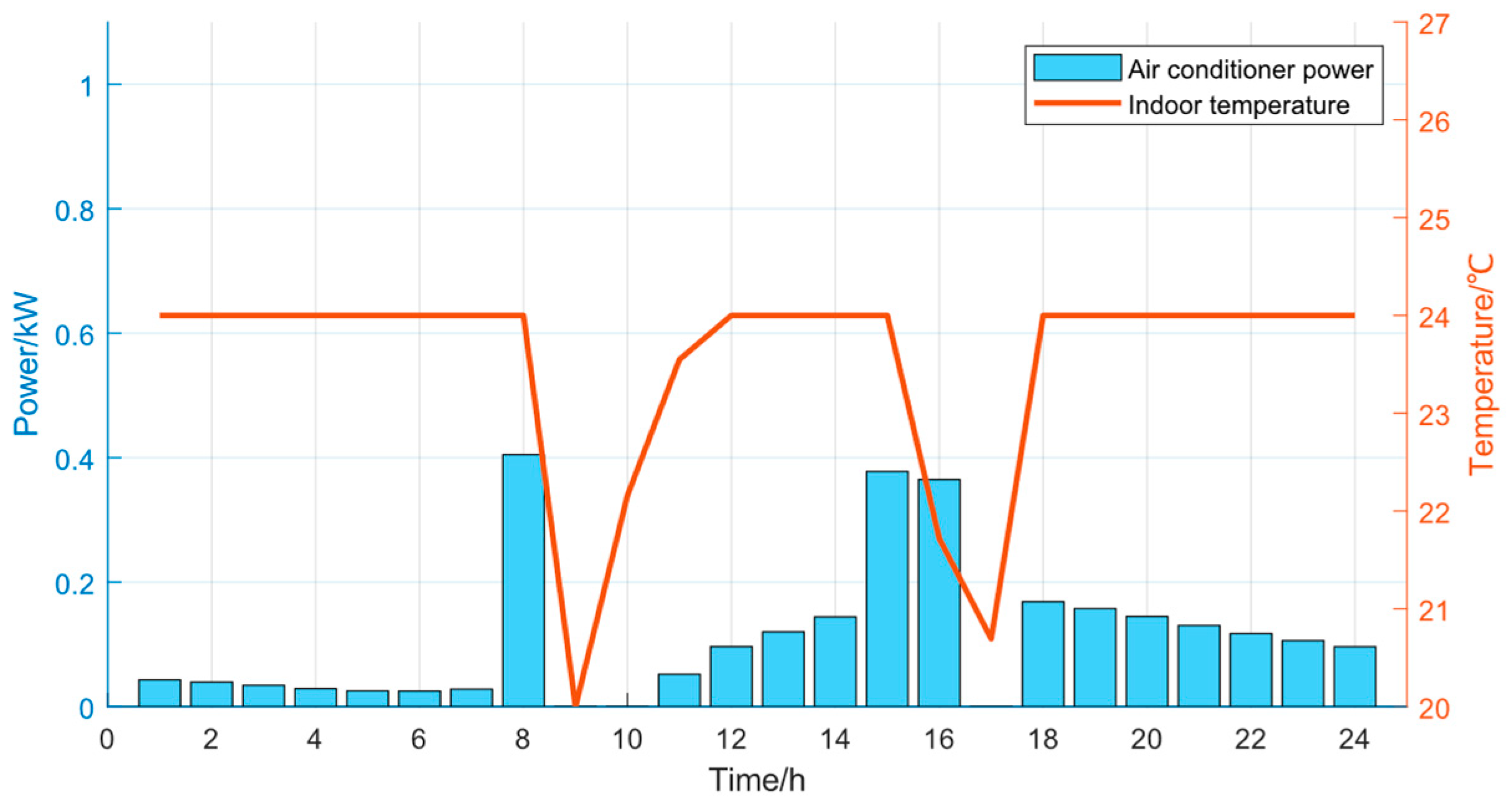
Scenario 3: Configuration of energy storage station and consideration of temperature-controlled load flexibility.

Figure 5 shows the behavior of the load power consumption and the amount of wind and light discarded in Scenario 1. From the figure, when the grid price is in the peak range, the load still purchases power from the grid, which significantly increases the cost of purchasing power. The data in the figure show that the grid price peaked at 18–20 h, when the power purchased from the grid was also higher. At other times of the day, such as 0–6 pm at night, grid tariffs were lower, but loads were not storing power or adopting other strategies to reduce costs during the low tariff hours. At the same time, the graph showed the presence of wind and light rejection. The amount of wind and light waste was more obvious during certain hours such as 12–14 h and at night. This not only results in a wastage of RE, but also leads to loads purchasing power from the grid during high price hours, which increases the overall cost of purchasing power.

Figure 6 presents the load power consumption behavior and the charging and discharging power of the ESS for Scenario 2. Compared with Scenario 1, the loads in Scenario 2 have the ability to store excess RE to the storage station. When there is a surplus of RE, the surplus can be further utilized by discharging from the storage station when the electricity price is in the peak period, thus significantly increasing the rate of RE consumption. At the same time, during 1:00–8:00, this grid price is in the valley of the time period, so the load will be from the grid with a large amount of purchased power. After meeting their own power needs, they will also sell the excess power to the storage station. The storage station then stores this power for discharge during the peak price period, thus making a profit on the price difference. In particular, the load’s behavior of purchasing electricity from the grid avoids the peak tariff periods, and during the two peak tariff periods of 9:00–12:00 and 17:00–21:00, the load chooses to purchase electricity from the storage station, which sells electricity at relatively low tariffs, which is in line with the load’s self-interest. Overall, the introduction of the ESS enables complementary energy utilization among different loads by leveraging the diverse and complementary characteristics of RE generation. This effectively reduces the annual operating costs of loads and significantly enhances the RE consumption rate.

Figure 7 illustrates the operating power and indoor temperature variation of the air conditioning system in Scenario 2. This scenario was defined as the baseline case, where the indoor temperature was maintained at a constant value and the flexibility of temperature-controlled loads was not considered. It was observed that the operating power of the air conditioning system was significantly influenced by the external ambient temperature; the greater the deviation between the outdoor temperature and the user’s comfort setpoint, the higher the air conditioning power consumption. Since the flexibility of the air conditioning system was not fully utilized in this scenario, a relatively fixed operating pattern was adopted without intelligent and efficient adjustment based on real-time environmental and demand variations, leading to a higher energy consumption and poorer economic performance.

Figure 8 illustrates the variation in the air conditioning power and room temperature over time in Scenario 3. In this scenario, the flexibility of temperature-controlled loads is fully exploited through the incorporation of a user-defined comfort temperature range. It was evident that room temperature was affected by both the external ambient temperature and air conditioning power. While ensuring that the room temperature remained within the user’s comfort range, a significant temperature drop occurred at 9:00 and 17:00. This occurred because electricity prices are higher at these two time points, prompting the air conditioning system to increase its operating power at 8:00 and 16:00 to pre-cool and store cold energy in advance. Leveraging the thermal dynamic properties of the building, this early cooling operation led to a decrease in room temperature at 09:00 and 17:00. By utilizing the flexibility of temperature-controlled loads, the energy consumption of the air conditioner is reduced during the peak tariff hours, which in turn reduces the cost of electricity used by the loads during the peak tariff periods. It can be seen that by rationally adjusting the power of the air conditioner and fully utilizing the flexibility of temperature-controlled loads, both the comfort of the indoor environment and the cost of electricity consumption can be guaranteed.

Table 1. Comparison of data across three scenarios (economic unit: CNY).

Scenario	Load Annual Operating Costs	Annual Net Income from Energy Storage Stations	RE Consumption Rate
1	12,996,483	—	86.7%
2	8,832,489	301,648	100%
3	8,624,186	324,349	100%

presents the annual operating costs, annual net returns of the ESS, and the RE consumption rate of the loads under the three scenarios. To further evaluate the impact of incorporating temperature-controlled load flexibility on the economic performance of the ESS, this paper compared the annual net return of the ESS. The annual net return is defined as the annual revenue of the ESS minus its annual investment and operation and maintenance costs.

Scenario 1 did not configure the energy storage power station and did not consider temperature-controlled load flexibility, the annual operating cost was CNY 12.996 million, and the RE consumption rate was 86.7%, leading to a significant curtailment of wind and solar energy and resulting in substantial resource waste.

Scenario 2 was configured with an ESS, but did not consider temperature-controlled load flexibility, with an annual operating cost of CNY 8.832 million and a RE consumption rate of 100%. Compared with Scenario 1, the annual operating cost of the load was saved by 32.05%, and the RE consumption rate was increased by 13.3%, which shows that the configuration of the energy storage station can significantly reduce the annual operating cost of the load and increase the RE consumption rate.

In Scenario 3, configuring the ESS and considering the flexibility of temperature-controlled loads, the annual operating cost was CNY 8.624 million, which is a saving of 2.35% compared with Scenario 2, and the annual net benefit of the ESS was improved by 7.64%. This indicates that considering temperature-controlled load flexibility can further improve the economics of the load and the ESS. The above comparison demonstrates that the configuration of the ESS enables complementary power consumption behavior of the load, enhances the utilization rate of RE, and reduces the annual operating cost of the load. Meanwhile, by considering the flexibility of temperature-controlled loads, the potential of the air conditioning can be fully utilized, further improving the economic efficiency of both the ESS and the loads. Additionally, investment in the construction of the ESS can yield substantial returns, demonstrating a viable profit margin.

In addition, it can be calculated that the annual revenue of the ESS in Scenario 3 was CNY 2.719 million, with a total configuration cost of CNY 20.074 million and an annual O&M cost of CNY 344,000. The static investment payback period of the ESS was 8.5 years, indicating a relatively considerable profit margin.

In order to more deeply verify the strengths of this paper’s approach, the adaptive scalar value of this paper’s method and several other methods were compared, as shown in Figure 9. The algorithms involved were as follows: Method 1 is the scheme proposed in this paper; method 2 stems from the POA algorithm without improvement; method 3 is based on the GWO algorithm without improvement; and method 4 is the POA-GWO algorithm without CSO improvement.

From the results in Figure 9, the fitness function value of method 1 (i.e., using the POA-GWO-CSO algorithm) was significantly higher than in the other schemes for the same number of iterations. This indicates that during the optimization process, the POA-GWO-CSO algorithm was able to explore the solution space more efficiently and converge quickly toward the optimal solution. Compared with the other compared algorithms, the algorithm could obtain better fitness values in fewer iterations, which indicates that it can find a solution that satisfies the multi-objective optimization at a faster speed, greatly reducing the computation time and resource consumption. This fast convergence and efficient solution feature is crucial in practical grid energy storage planning applications, and enables grid operators to make accurate and cost-effective decisions quickly when facing complex power supply and energy storage allocation problems, fully demonstrating the significant superiority of the POA-GWO-CSO algorithm in solving the multi-objective optimization problem of grid energy storage.

7. Conclusions

This paper proposed a multi-objective optimal allocation method of a grid ESS taking into account the flexibility of temperature-controlled loads, and the results showed the following:

(1)

This paper incorporated the energy storage station into the grid model, which not only guarantee the balanced operation of the grid, but also enhances the consumption of RE. At the same time, it fully exploits the flexibility of temperature-controlled loads and integrates them into the grid storage power station model, which reduces the cost of electricity on the basis of guaranteeing the comfort of the indoor environment.

(2)

The multi-objective optimization strategy for the grid ESS proposed in this paper not only improved the utilization efficiency of energy storage resources and enhanced the overall benefits of the system, but also obtained the scheme that minimized the operating costs of the grid and the configuration costs of the ESS. The results indicate that compared with Scenarios 1 and 2, the operating costs in Scenario 3 were reduced by 33.6% and 2.35%, respectively. Furthermore, the revenue of the energy storage station in Scenario 3 was 7.6% higher than that in Scenario 2.

(3)

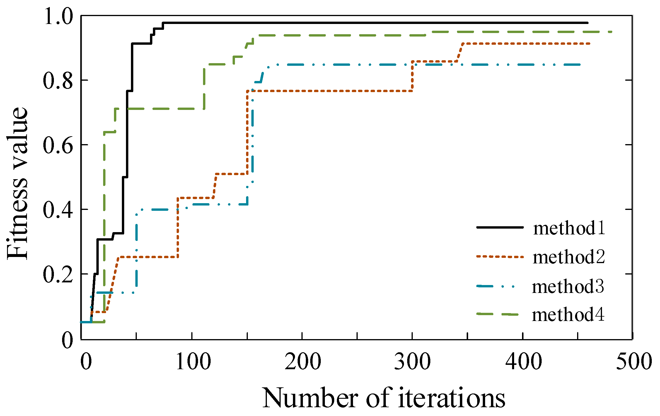
The POA-GWO-CSO algorithm employed in this paper efficiently solved the multi-objective optimization problem of grid energy storage, thereby enhancing the optimization and allocation efficiency of the energy storage system while reducing the decision-making time.

In future work, for Scenario 2, additional terms will be incorporated into the objective function, such as power fluctuation smoothing terms and state-of-charge variation penalty terms, in order to balance economic performance and system flexibility while alleviating the stress on the distribution network caused by concentrated load fluctuations. Moreover, future studies are expected to introduce stochastic and uncertainty modeling of renewable energy sources to enable a more detailed analysis of grid scalability, load characteristic curve evolution, and the stochastic fluctuations of renewable energy outputs. These enhancements will contribute to the development of a more resilient system planning and operational framework, particularly under conditions of high renewable energy penetration and increasing load uncertainty, thereby improving the overall adaptability and reliability of the system.

References

1. Li, J.; Fang, Z.; Wang, Q.; Zhang, M.; Li, Y.; Zhang, W. Optimal Operation with Dynamic Partitioning Strategy for Centralized Shared Energy Storage Station with Integration of Large-scale RE. J. Mod. Power Syst. Clean Energy 2024, 12, 359–370. [Google Scholar] [CrossRef]
2. Abomazid, A.M.; El-Taweel, N.A.; Farag, H.E.Z. Optimal Energy Management of Hydrogen Energy Facility Using Integrated Battery Energy Storage and Solar Photovoltaic Systems. IEEE Trans. Sustain. Energy 2022, 13, 1457–1468. [Google Scholar] [CrossRef]
3. Hou, H.; Chen, Y.; Liu, P.; Xie, C.; Huang, L.; Zhang, R.; Zhang, Q. Multisource Energy Storage System Optimal Dispatch Among Electricity Hydrogen and Heat Networks from the Energy Storage Operator Prospect. IEEE Trans. Ind. Appl. 2021, 58, 2825–2835. [Google Scholar] [CrossRef]
4. Hossain, M.B.; Islam, M.R.; Muttaqi, K.M.; Sutanto, D.; Agalgaonkar, A.P. Component Sizing and Energy Management for a Supercapacitor and Hydrogen Storage Based Hybrid Energy Storage System to Improve Power Dispatch Scheduling of a Wind Energy System. IEEE Trans. Ind. Appl. 2024, 61, 872–883. [Google Scholar] [CrossRef]
5. Zhuang, Y.; Li, Z.; Tan, Q.; Li, Y.; Wan, M. Multi-Time-Scale Resource Allocation Based on Long-Term Contracts and Real-Time Rental Business Models for Shared Energy Storage Systems. J. Mod. Power Syst. Clean Energy 2024, 12, 454–465. [Google Scholar] [CrossRef]
6. Islam, M.M.; Yu, T.; Giannoccaro, G.; Mi, Y.; La Scala, M.; Rajabi, M.N.; Wang, J. Improving Reliability and Stability of the Power Systems: A Comprehensive Review on the Role of Energy Storage Systems to Enhance Flexibility. IEEE Access 2024, 12, 152738–152765. [Google Scholar] [CrossRef]
7. Han, J.; Fang, Y.; Li, Y.; Du, E.; Zhang, N. Optimal Planning of Multi-Microgrid System with Shared Energy Storage Based on Capacity Leasing and Energy Sharing. IEEE Trans. Smart Grid 2024, 16, 16–31. [Google Scholar] [CrossRef]
8. Kong, W.; Sun, K.; Zhao, J. Two-stage Optimal Scheduling of Community Integrated Energy System Considering Operation Sequences of Hydrogen Energy Storage Systems. J. Mod. Power Syst. Clean Energy 2025, 13, 276–288. [Google Scholar] [CrossRef]
9. Guo, Z.; Wei, W.; Shahidehpour, M.; Chen, L.; Mei, S. Two-Timescale Dynamic Energy and Reserve Dispatch with Wind Power and Energy Storage. IEEE Trans. Sustain. Energy 2022, 14, 490–503. [Google Scholar] [CrossRef]
10. Zhang, H.; Li, Z.; Xue, Y.; Chang, X.; Su, J.; Wang, P.; Guo, Q.; Sun, H. A stochastic bi-level optimal allocation approach of intelligent buildings considering energy storage sharing services. IEEE Trans. Consum. Electron. 2024, 70, 5142–5153. [Google Scholar] [CrossRef]
11. Zhai, X.; Li, Z.; Li, Z.; Xue, Y.; Chang, X.; Su, J.; Jin, X.; Wang, P.; Sun, H. Risk-averse energy management for integrated electricity and heat systems considering building heating vertical imbalance: An asynchronous decentralized approach. Appl. Energy 2025, 383, 125271. [Google Scholar] [CrossRef]
12. Lu, J.; Zheng, W.; Yu, Z.; Xu, Z.; Jiang, H.; Zeng, M. Optimizing Grid-Connected Multi-Microgrid Systems with Shared Energy Storage for Enhanced Local Energy Consumption. IEEE Access 2024, 12, 13663–13677. [Google Scholar] [CrossRef]
13. Zhang, H.; Zhou, S.; Gu, W.; Zhu, C.; Chen, X.G. Optimal Operation of Micro-energy Grids Considering Shared Energy Storage Systems and Balanced Profit Allocations. CSEE J. Power Energy Syst. 2022, 9, 254–271. [Google Scholar]
14. Wang, G.; Wang, C.; Feng, T.; Wang, K.; Yao, W.; Zhang, Z. Day-Ahead and Intraday Joint Optimal Dispatch in Active Distribution Network Considering Centralized and Distributed Energy Storage Coordination. IEEE Trans. Ind. Appl. 2024, 60, 4832–4842. [Google Scholar] [CrossRef]
15. Qi, C.; Wang, K.; Fu, Y.; Li, G.; Han, B.; Huang, R.; Pu, T. A decentralized optimal operation of AC/DC hybrid distribution grids. IEEE Trans. Smart Grid 2017, 9, 6095–6105. [Google Scholar] [CrossRef]
16. Lu, X.; Liu, Z.; Hu, J.; Xiao, C.; Feng, K.; Jin, W. Optimization method for multi-port alternating current/direct current flexible integrated energy control systems based on improved pelican optimization algorithm. Renew. Energy 2024, 42, 1697–1706. [Google Scholar]
17. Gan, L.; Low, S.H. Optimal power flow in direct current networks. IEEE Trans. Power Syst. 2014, 29, 2892–2904. [Google Scholar] [CrossRef]
18. Nagpal, H.; Avramidis, I.-I.; Capitanescu, F.; Madureira, A.G. Local Energy Communities in Service of Sustainability and Grid Flexibility Provision: Hierarchical Management of Shared Energy Storage. IEEE Trans. Sustain. Energy 2022, 13, 1523–1535. [Google Scholar] [CrossRef]
19. Yang, W.; Song, L. A Two-Stage Investment Behavior-Based Approach for Efficient Allocation of Electrical Energy with Shared Energy Storage Station. IEEE Access 2024, 12, 105148–105164. [Google Scholar] [CrossRef]
20. Yan, D.; Chen, Y. Distributed Coordination of Charging Stations with Shared Energy Storage in a Distribution Network. IEEE Trans. Smart Grid 2023, 14, 4666–4682. [Google Scholar] [CrossRef]
21. Xia, S.; Cai, L.; Tong, M.; Wu, T.; Li, P.; Gao, X. Regulation Flexibility Assessment and Optimal Aggregation Strategy of Greenhouse Loads in Modern Agricultural Parks. Prot. Control Mod. Power Syst. 2024, 9, 98–111. [Google Scholar] [CrossRef]
22. Wang, P.; Wu, D.; Kalsi, K. Flexibility Estimation and Control of Thermostatically Controlled Loads with Lock Time for Regulation Service. IEEE Trans. Smart Grid 2020, 11, 3221–3230. [Google Scholar] [CrossRef]
23. Hao, H.; Wu, D.; Lian, J.; Yang, T. Optimal Coordination of Building Loads and Energy Storage for Power Grid and End User Services. IEEE Trans. Smart Grid 2017, 9, 4335–4345. [Google Scholar] [CrossRef]
24. Chen, H.; Xiong, X.; Zhu, J.; Wang, J.; Wang, W.; He, Y. A Two-Stage Stochastic Programming Model for Resilience Enhancement of Active Distribution Networks with Mobile Energy Storage Systems. IEEE Trans. Power Deliv. 2023, 39, 2001–2014. [Google Scholar] [CrossRef]
25. Bai, W.; Wang, D.; Sun, X.; Yu, J.; Xu, J.; Pan, Y. An Online Multi-Level Energy Management System for Commercial Building Microgrids with Multiple Generation and Storage Systems. IEEE Open Access J. Power Energy 2023, 10, 195–207. [Google Scholar] [CrossRef]
26. Wu, S.; Li, Q.; Liu, J.; Zhou, Q.; Wang, C. Bi-level optimal configuration for combined cooling heating and power multi-microgrids based on energy storage station service. Power Syst. Technol. 2021, 45, 3822–3829. [Google Scholar]
27. Wen, K.; Li, W.; Han, S.; Jin, C.; Zhao, Y. Optimization of deployment with control for battery energy storage system participating in primary frequency regulation service considering its calendar life. High Volt. Eng. 2019, 45, 2185–2193. [Google Scholar]
Figure 1. Operational framework for ESS in the power grid.
Energies 18 02527 g001
Figure 2. POA-GWO-CSO algorithm flow diagram.
Energies 18 02527 g002
Figure 3. Outdoor light intensity and temperature curve.
Energies 18 02527 g003
Figure 4. Maximum forecasted output data for the photovoltaic and wind power and conventional load curves.
Energies 18 02527 g004
Figure 5. Scenario 1: Load power consumption behavior and the amount of wind and solar energy abandonment.
Energies 18 02527 g005
Figure 6. Scenario 2: Load power consumption behavior and charging/discharging power of the ESS.
Energies 18 02527 g006
Figure 7. Air conditioner operation power and temperature change in room of Scenario 2.
Energies 18 02527 g007
Figure 8. Air conditioner operation power and temperature change in room of Scenario 3.
Energies 18 02527 g008
Figure 9. Scaled value of fitness for different algorithms.
Energies 18 02527 g009