Future Smart Grids Control and Optimization: A Reinforcement Learning Tool for Optimal Operation Planning

Abstract

The smart grids of the future present innovative opportunities for data exchange and real-time operations management. In this context, it is crucial to integrate technological advancements with innovative planning algorithms, particularly those based on artificial intelligence (AI). AI methods offer powerful tools for planning electrical systems, including electrical distribution networks. This study presents a methodology based on reinforcement learning (RL) for evaluating optimal power flow with respect to various cost functions. Additionally, it addresses the control of dynamic constraints, such as voltage fluctuations at network nodes. A key insight is the use of historical real-world data to train the model, enabling its application in real-time scenarios. The algorithms were validated through simulations conducted on the IEEE 118-bus system, which included five case studies. Real datasets were used for both training and testing to enhance the algorithm’s practical relevance. The developed tool is versatile and applicable to power networks of varying sizes and load characteristics. Furthermore, the potential of RL for real-time applications was assessed, demonstrating its adaptability to online grid operations. This research represents a significant advancement in leveraging machine learning to improve the efficiency and stability of modern electrical grids.

1. Introduction

The transition to future smart grids marks a fundamental transformation shift in energy management, especially when enhanced by advanced digital technologies, artificial intelligence (AI), and the Internet of Things (IoT) [1,2]. These innovations aim to improve efficiency, reliability, and sustainability. Unlike traditional power systems, smart grids feature real-time monitoring, self-healing mechanisms, and decentralized power generation from renewable sources. Most importantly, they enable decentralized forms of control.

Networks designed in this manner facilitate the seamless integration of distributed energy resources (DER) with load flexibility management systems. Achieving this integration relies on the effective use of strategic planning and optimal power flow optimal power flow (OPF) techniques. Strategic planning ensures the successful incorporation of DER, renewable energy sources (RESs), and demand management, while also optimizing grid expansion and infrastructure upgrades. Conversely, OPF techniques identify the most efficient energy distribution strategies by minimizing generation costs and transmission losses while maintaining system stability.

For many years, OPF techniques have been essential tools for the efficient planning and operation of electrical systems [3,4]. The goal of this methodology is to determine the most optimal or stable operating point to meet specific cost function objectives while adhering to system constraints. Generally, OPF objectives can be categorized into two types: single-objective minimization and multi-objective minimization [5,6,7].

When discussing traditional methods for solving the optimal power flow (OPF) problem, we can identify two main categories of algorithms: deterministic and stochastic [8]. The deterministic category encompasses linear and non-linear programming, gradient methods (GM), Newton’s method (NM), and interior point methods (IPM) [4,9]. These algorithms rely on specific assumptions regarding the convexity, regularity, continuity, and differentiability of the cost function. Generally, they are quite effective and quick when the cost function is monotonic. However, in modern power networks, cost functions often exhibit quadratic characteristics or non-linearity. This non-linearity affects the input-output behaviors of generating units, resulting in fuel costs that are both non-linear and non-smooth [10].

To tackle these challenges, several methods have been developed over the years based on metaheuristic techniques [3,11,12]. Among the most well-known of these are the genetic algorithm (GA), particle swarm optimization (PSO), and the artificial bee colony (ABC) algorithm [9,13]. Although these methods frequently achieve convergence, they tend to involve a significant computational burden [14]. In terms of the content of future smart grids, it is necessary to look at new approaches based also on Artificial Intelligence, so other approaches are also becoming popular. In this context, reinforcement learning (RL) has been employed to address various real-world control and decision-making challenges in uncertain scenarios. However, its utilization in power system management has been limited [15].

For instance, in [16], an OPF methodology based on Deep Q-Network (DQN) was developed for a network under different loading conditions. In [17], an RL algorithm was devised to address the AC OPF problem based on proximal policy optimization (PPO). The same authors presented a similar methodology in [18] applying RL considering several topology changes. The paper uses an offline training method to correctly initialize the parameters of the neural networks (NNs). Although this leads to a considerable improvement in performance, it also introduces an element of great complexity that impacts the reproducibility of the algorithm. For this reason, in this work, an effort has been made to develop a model that does not require pre-training. A common approach, often used due to the scarcity of datasets, is to perturb load values around their nominal value [17,19]. However, this method is highly limiting, as it fails to account for extreme load conditions, which at certain hours of the day can drop to zero. In [20,21], the authors developed an algorithm based on twin delayed deep deterministic policy gradient (TD3) while considering random load distributions. In this case, the results are presented in an aggregated form, preventing a clear assessment of the RL actual performance. Another approach is the one presented in [22] where constant loads are used. Finally, in [8], RL is employed using PPO to solve an OPF to minimize power losses. In [23], the authors propose a distributed optimal power flow RL-based model which is highly effective when there is a large number of RESs. The main gaps that this article aims to address concern the definition of reward functions that can be of general value for even complex planning scenarios and the possibility of training based on historical data. In this way, the system can create models that can be used to make decisions in real time. The idea is to create a model that learns from real data obtained historically and the network thus driven can be used to react in real time to what happens in the network. Observations are possible because smart grids can measure and exchange information. Starting from these considerations this paper aims to develop a methodology, that learns for the solution of OPF problem and learns how to map the observation on action that can satisfy the cost function. The issue discussed in the paper is that the inclusion of RESs increases the uncertainty in the network, making the optimization problem more challenging and realistic. Unlike traditional methods that primarily focus on quadratic cost functions, this study examines more practical cost formulations that take into account voltage state analysis at various nodes. Additionally, the paper provides comparative assessments with meta-heuristic models, showcasing the effectiveness of the proposed method. A great deal of work has been done on creating the framework, cost functions, and training methodologies, leaving the TD3 algorithm in its classic form to demonstrate the possibilities of standard approaches to solving the problem.

The key contributions of this paper can be summarized as follows:

• Formulating the OPF problem as an original Markov decision process (MDP) to be solved using RL.
• Using real datasets for training, and validation, incorporating both load and renewable generation data.
• Exploring advanced cost functions beyond traditional quadratic formulations, including voltage state analysis at different nodes.
• Providing a replicable tool for electrical networks of varying sizes and load characteristics.
• Comparing the proposed approach with traditional methods to validate it.

The paper is organized as follows: Section 2 provides the key principles of RL and describes the utilized algorithm. Section 3 outlines the formulation of the AC OPF problem. Section 4 presents the structure of the Data-Driven based AC OPF solver. Section 5 showcases the results obtained from testing the algorithm on the target network. Finally, Section 6 contains conclusions and remarks on future work.

2. RL Principles and TD3 Algorithm

2.1. Principles of RL

RL is a machine learning (ML) paradigm that focuses on learning how to act optimally in an environment through a trial-and-error approach (Figure 1 shows the main working principles). A fundamental aspect of RL lies in its dependency on the Markov property. It asserts that the current states solely determine the future states of the system. The intelligent decision-maker, often referred to as the agent, interacts with elements external to it, namely the environment. The agent interacts with the environment by taking actions a, and these actions result in rewards r, typically represented as numerical values, which indicate the quality of the agent’s decisions. Positive rewards are associated with favorable actions, while negative rewards correspond to unwanted ones. The positions assumed by the agent in the environment are known as states s. When the agent, at time step t, performs an action, it receives a reward and moves from state $s_t$ to state $s_{t+1}$.

The agent’s behavior in an environment is dictated by the policy, which instructs the agent on which action to take. Policies can be either deterministic, $\mu \left(a_t\right|s_t)$, or stochastic, $\pi \left(a_t\right|s_t)$. The movement from one state to another is called a transition, which is characterized by a certain probability. This process enables the agent to learn and improve its decision-making over time. The occurrence of states, transition probability, actions, and rewards thus defines an MDP. The agent interacts with the environment starting from the initial state until it reaches the final one. This interaction is called an episode. The final goal of RL is to learn which actions yield the highest discounted sum of rewards, namely the cumulative reward $G_t$.

$$G_t\doteq R_{t+1}+\gamma R_{t+2}+{\gamma }^2{R}_{t+3}+\dots =\sum _{k=0}^{\infty }{\gamma }^k{R}_{t+k+1}$$

(1)

where $R_t$ is the reward at time t and $0<\gamma \le 1$ is the discount factor.

Two important concepts for assessing the value of an agent in a particular state are the value function and the action value function (Q-function). The first expresses the expected return starting from a state s and following the policy $\pi$ over a given time horizon. The latter represents the expected cumulative reward that an agent can achieve by taking a specific action a in a given state s and following a particular policy $\pi$. For MDPs they are expressed as in (2) and (3):

$$v_{\pi }\left(s\right)\doteq {\mathbb{E}}_{\pi }\left[G_t\right|S_t=s]$$

(2)

$$\begin{array}{cc}\hfill q_{\pi }(s,a)& \doteq {\mathbb{E}}_{\pi }\left[G_t\right|S_t=s,A_t=a]\hfill \end{array}$$

(3)

Here $\mathbb{E}$ is the expected return. Both for (2) and (3) it is possible to define an equation that expresses a relationship between the value of a state and the values of its possible successor states, namely the Bellman equation.

$$\begin{array}{c}\hfill v_{\pi }\left(s\right)=\sum _a\pi \left(a\right|s)\sum _{s^{\prime },r}p(s^{\prime },r|s,a)\left[r+\gamma v_{\pi }\left(s^{\prime }\right)\right]\end{array}$$

(4)

Based on what has been stated, the condition for finding the optimal policy is computing the optimal value function $v_{*}$. The optimal policy ${\pi }_{*}$ is then recovered by picking up an action that is greedy with respect to $v_{*}$:

$$\begin{array}{cc}\hfill v_{*}\left(s\right)& \doteq \underset{\pi }{max}{v}_{\pi }\left(s\right)\hfill \end{array}$$

(5)

Similarly, for the optimal action value function $q_{*}$:

$$\begin{array}{cc}\hfill q_{*}(s,a)& \doteq \underset{\pi }{max}{q}_{\pi }(s,a)\hfill \end{array}$$

(6)

The entire discussion concerning RL principles relies on theory and notations outlined in [24,25].

2.2. RL Algorithms

RL methods can be classified as value-based, policy-based and actor-critic. The first class of algorithms computes the optimal Q-value iteratively, using the Bellman equation, and then extracts the optimal policy. TD-learning, SARSA and Q-learning are the most famous algorithms of this class. They are called table methods, since they store value and Q-value functions in lookup tables. This is very limiting when the state and action spaces are vast. This is why deep Q-network (DQN) was introduced. It is a variant of Q-learning where Q-values are approximated by using deep neural networks. Basically, the Q-function is parameterized by $\theta$, leading to $q_{\theta }(s,a)$, where $\theta$ represents the vector of parameters used to approximate the Q function. These parameters include the weights and biases of a neural network if a NN is used to approximate the Q function, or other parameters if alternative approximation techniques are used. The combination of deep learning (DL) and RL thus leads to the so-called deep reinforcement learning (DRL) where the agent update the NN parameters to achieve the optimal policy. One of the disadvantages of this class of algorithms is that they are suitable only for environments with a discrete action space and can not be applied to continuous environments. This is why a second class of algorithms, called policy-based methods, was introduced. They leverage on the policy gradient method to find the optimal parameter $\theta$ of the NN to obtain the correct probability distribution over the action space. Thus, the goal of the network is to assign high probabilities to actions that maximize the cumulative reward of a trajectory $\tau$. Therefore, the objective function J can be expressed as:

$$J\left(\theta \right)={\mathbb{E}}_{\tau \sim {\pi }_{\theta }\left(\tau \right)}\left[G\left(\tau \right)\right]$$

(7)

Here, $\tau \sim {\pi }_{\theta }\left(\tau \right)$ indicates that the trajectory $\tau$ is sampled according to the policy ${\pi }_{\theta }$, which is defined by the network. The objective function is maximized by computing the gradient and updating the parameters according to:

$$\theta =\theta +\alpha {\nabla }_{\theta }J\left(\theta \right)$$

(8)

where $\alpha$ is the learning rate. Another class of methods lies on the intersection of policy-based and value-based methods. It is called the actor critic (AC) method. It consists of two types of NN, the actor-network and the critic network. The role of the first one is to find the optimal policy while the other one evaluates the policy produced by the actor. In AC the parameters are updated at each and every step of the episode. One of the most famous algorithms is called deep deterministic policy gradient (DDPG). It is an off-policy, model-free algorithm that works in continuous action spaces. DDPG uses the policy network as an actor and DQN as a critic. It works with a deterministic policy instead of a stochastic one.

2.3. TD3 Algorithm

In this paper, simulations are performed considering a more powerful and stable variant of DDPG, called TD3. The pseudocode of the algorithm is reported in Algorithm 1 [25].

Algorithm 1 TD3 algorithm

1:  Initialize the 2 main critic network parameters ${\theta }_1$ and ${\theta }_2$ and the main actor network parameter $\varphi$ 2:  Initialize the 2 target critic network parameters ${\theta }_1^{\prime }$ and ${\theta }_2^{\prime }$ by copying ${\theta }_1$ and ${\theta }_2$ 3:  Initialize the target actor network parameter ${\varphi }^{\prime }$ by copying $\varphi$ 4:  Initialize the replay buffer $\mathcal{D}$ 5:  for $episode:1$ to n do 6:      for $step$ $t:1$ to $T-1$ do 7:         select action a based on the deterministic policy ${\mu }_{\varphi }\left(s\right)$ with exploration noise $ϵ$, that is:         $a={\mu }_{\varphi }\left(s\right)+ϵ$, where $ϵ\sim \mathcal{N}(0,\sigma )$ 8:         perform action a, move to next state $s^{\prime }$, get a reward r and store the transition information in the buffer $\mathcal{D}$ 9:         select action $\tilde{a}$ to compute the target value, that is:         $\tilde{a}={\mu }_{\varphi }\left(s_i^{\prime }\right)+ϵ$, where $ϵ\sim \mathcal{N}(0,\sigma ,-c,c)$ 10:       compute the target value of the critic network, that is:       $y_i=r_i+\gamma \underset{j=1,2}{min}{Q}_{{\theta }_j^{\prime }}(s_i^{\prime },\tilde{a})$ 11:       compute the loss function of the critic network, that is:       $L_{{\theta }_j}={\displaystyle \frac{1}{K}}{\sum }_{i=1}^K{(y_i-Q_{{\theta }_j}(s_i,a_i))}^2$    for $j=1,2$ 12:       compute the gradient of the loss function, that is:       ${\nabla }_{{\theta }_j}J\left({\theta }_j\right)$ 13:       minimize the loss using gradient descent and then update the parameters, that is:       ${\theta }_j={\theta }_j-\alpha {\nabla }_{{\theta }_j}L\left({\theta }_j\right)$    for $j=1,2$ 14:       if t mod $d=0$ then 15:          - compute the gradient of the objective function ${\nabla }_{\varphi }J\left(\varphi \right)$ and update the actor network parameter using gradient ascent, $\varphi =\varphi +-\alpha {\nabla }_{\varphi }J\left(\varphi \right)$ 16:        - update the target critic network parameter and target actor network parameter as $\theta j^{\prime }=\tau {\theta }_j+(1-\tau ){\theta }_{j}i$, for $j=1,2$ and ${\varphi }^{\prime }=\varphi +-\alpha {\nabla }_{{\varphi }^{\prime }}J\left({\varphi }^{\prime }\right)$, respectively 17:         end if 18:     end for 19: end for

3. Problem Formulation

As previously mentioned, the goal of the OPF is to find the optimal generator set-points such that a cost function is minimized while satisfying system and security constraints. The control variables of the AC OPF are the active power generation at the PV buses (slack bus excluded), the voltage magnitude of PV buses, the tap settings of transformers and the eventual shunt VAR compensation. On the other side, the state variables are the active power of the slack bus, the voltage magnitude of PQ buses, the reactive power of all generators and the transmission line loadings. The PQ buses are voltage and reactive power-controlled buses, the PV buses are voltage and active power-controlled buses, and the slack bus is the reference bus that acts as a compensator. In the present paper, both the tap settings and VAR compensation are neglected. Generally, the basic cost function is the total generating fuel cost; each generator has its own cost curve represented by a quadratic function. In this case, given a set of buses N, a subset of generator buses G, load demand buses D and a set of transmission lines L, the OPF problem can be formulated as [3]:

• Objective function

$$min\sum _{i\in G}\underset{{\mathrm{CF}}_{1i}}{\underbrace{\left(c_{0i}+c_{1i}{P}_{\mathrm{g}i}+c_{2i}{P}_{\mathrm{g}i}^2\right)}}\equiv min\sum _{i\in G}{\mathrm{CF}}_{1i}$$

(9)

• Equality constraints

$$P_j=|V_j|\sum _{i\in N}\left|V_i\right|(g_{ji}cos({\delta }_j-{\delta }_i)+b_{ji}sin({\delta }_j-{\delta }_i))\forall j\in N$$

(10)

$$Q_j=|V_j|\sum _{i\in N}\left|V_i\right|(g_{ji}sin({\delta }_j-{\delta }_i)-b_{ji}cos({\delta }_j-{\delta }_i))\forall j\in N$$

(11)

• Inequality constraints

$$\begin{array}{c}\hfill P_{\mathrm{g}i}^{\min }\le P_{\mathrm{g}i}\le P_{\mathrm{g}i}^{\max }\forall i\in G\end{array}$$

(12)

$$\begin{array}{c}\hfill Q_{\mathrm{g}i}^{\min }\le Q_{\mathrm{g}i}\le Q_{\mathrm{g}i}^{\max }\forall i\in G\end{array}$$

(13)

$$\begin{array}{c}\hfill V_j^{\min }\le \left|V_j\right|\le V_j^{\max }\forall j\in N\end{array}$$

(14)

$$\begin{array}{c}\hfill |S_{{\mathrm{line}}_l}|\le S_{{\mathrm{line}}_l}^{\max }\forall l\in L\end{array}$$

(15)

where $c_0$, $c_1$ and $c_2$ are the cost coefficients of the ith generator. V is the bus voltage. $P_j$ and $Q_j$ are the net active and reactive power injections at bus j. The parameters $g_{ji}$ and $b_{ji}$ represent the conductance and susceptance between bus j and i while ${\delta }_i$ and ${\delta }_j$ are voltage angles at bus i and j respectively. Finally, $S_{lin{e}_l}$ represents the transmission line load of the l line [17]. Regarding the cost function, it is important to emphasize that the network may consider generators operating with different types of fuel. This leads to the function being divided into piecewise continuous quadratic cost functions. Furthermore, to make the function multi-objective, additional terms can be integrated into the quadratic fuel cost function. For instance, to obtain more accurate modelling of the cost function for multi-valve steam turbines, the so-called valve point effect can be considered. When the turbine operates at a valve point, just before the next valve opens, it operates at full efficiency. However, when the turbine operates off a valve point, it works less efficiently due to throttling losses. This effect significantly alters the output of the gas turbine, generating some ripples in the cost function. To account for this effect, a non smooth and non-convex rectified sine function can be added to the quadratic cost function, as detailed in (16) [11,12].

$${\mathrm{CF}}_2=\sum _{i\in G}{\mathrm{CF}}_{1i}+\left|c_{3i}·sin\left(c_{4i}·\left(P_{\mathrm{g}i}^{\min }-P_{\mathrm{g}i}\right)\right)\right|$$

(16)

where $c_3$ and $c_4$ are two coefficients that take into account the valve point effect.

Additionally, a component accounting for the voltage deviation from the unit at PQ buses can be included, aiming to improve the voltage profile of the entire system [3] as in (17).

$${\mathrm{CF}}_3=\sum _{i\in G}{\mathrm{CF}}_{1i}+{\lambda }_{\mathrm{VD}}·\left(\sum _{j\in N}|V_j-1|\right)$$

(17)

where ${\lambda }_{\mathrm{VD}}$ is a scaling factor to balance between the objective function values and to avoid the dominance of one objective over another.

In pursuit of a more comprehensive scenario, (16) and (17) can be merged. The function derived in this manner integrates both the valve point effect and voltage fluctuation control and thus all the complexities of the issue at hand

$${\mathrm{CF}}_4={\mathrm{CF}}_2+{\lambda }_{\mathrm{VD}}·\left(\sum _{j\in N}\left|V_j-1\right|\right)$$

(18)

In this research, all four cost functions will be taken into consideration. These will be minimized, considering the operational constraints, through the utilization of an offline-trained DRL agent and subsequently tested in real case scenarios.

4. DRL-Based AC-OPF

To address the AC-OPF problem with RL, it is necessary to model it as an MDP. In other words, starting from a time instant t, the DRL agent must make a decision $a_t$ based on observations of the current state of the environment. This leads to obtaining a reward $r_t$, which is useful to evaluate the quality of actions, and transition to the state $s_{t+1}$. This section describes the components of the aforementioned MDP: state-action space, reward function, environment, and agent.

4.1. State-Action Space

The states $s_t$ represent the initial input of the DRL agent. These states encompass the active and reactive power of loads at each bus. These are the observations considered by the agent to perform the actions. The state space can be summarized as in (19):

$$s=[P_{d1},...,P_{dn},Q_{d1},...,Q_{dn}]\forall n\in D$$

(19)

where n is the number of loads in the grid. On the other hand, actions $a_t$ involve the power output of each generator and its voltage setpoint.

$$a=[P_{g1},...,P_{gi},V_{g1},...,V_{gi}]\forall i\in G$$

(20)

4.2. Reward Function

The cost function $r_t$ assigns a reward every time an action $a_t$ is taken in a state $s_t$. As previously mentioned, in this paper the intent is to solve the optimal power flow (OPF) problem considering a multi-objective scenario. Initially $r_t$ is set equal to ${\mathrm{CF}}_1$, then ${\mathrm{CF}}_2$, ${\mathrm{CF}}_3$, and finally ${\mathrm{CF}}_4$. In this way, it is possible to observe the changes in the accuracy and performances of the RL algorithm moving from a single to a multi-objective cost function.

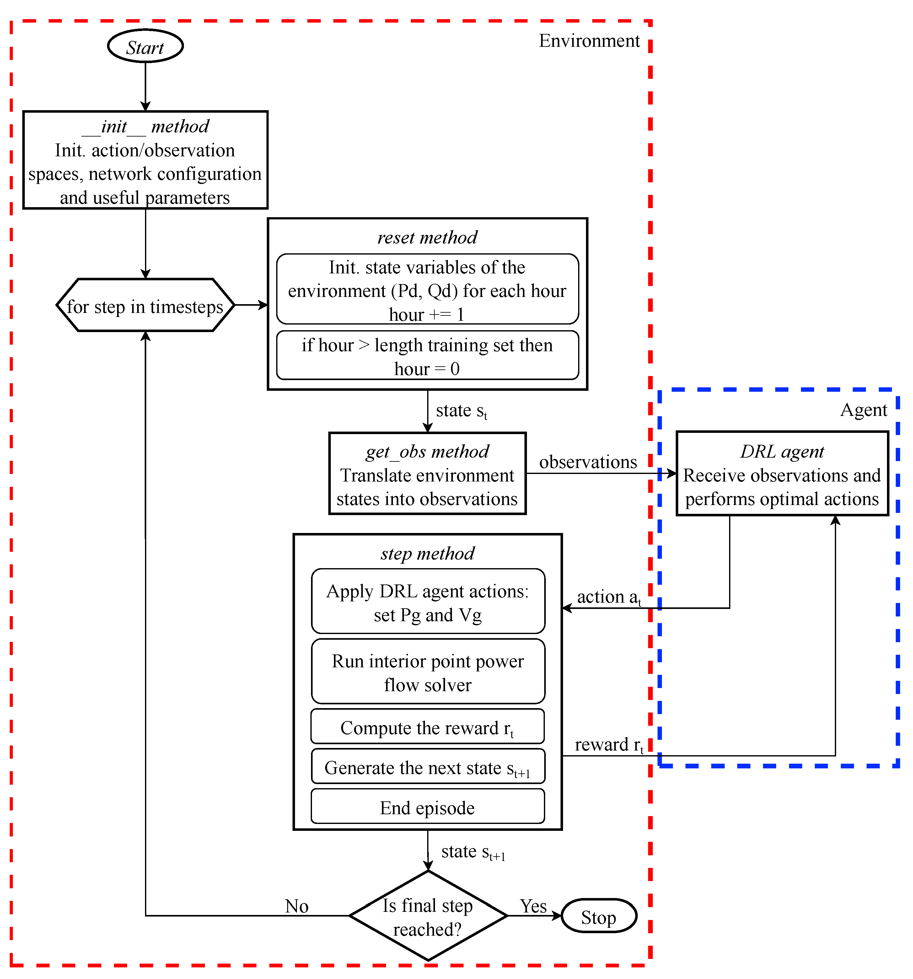
4.3. Environment

The development and structure of the custom environment used to model the MDP problem follows the conventions established by the OpenAI Gym library [26].

• Initialization (init method): It is used to establish the initial state, the action space, the observation space, and other environment-specific properties. It is executed once when the environment is created.
• Reset Function (reset method): The reset method is responsible for preparing the environment for a new episode. It returns the initial observation and sets the state to the starting configuration.
• Step Function (step method): The core of the custom environment is the step method. This method takes an action as input, updates the environment state, and returns critical information such as the next state, reward, and an indication of whether the episode is complete.
• Observation Retrieval (get obs): Involves obtaining observations of the current state after each action, crucial for guiding an agent’s decision-making process.

Additionally, it leverages the Pandapower library for modeling and solving power system-related aspects such as running the PF and building the network. The specific flowchart of the OpenAI Gym-based custom environment and its interaction with the RL agent is summarized in Figure 2.

4.4. DRL Agent and Training Process

As previously mentioned the algorithm used for training the agent is TD3. Specifically, the agent is trained using real load profiles with episodes of unit length. At the beginning of the episode, the reset method sets the loads values in hour h to the corresponding values of the dataset. Now the index h is used instead of index t for clarity of notation since a timestep corresponds to a specific hour. The agent then generates actions for the environment, leading to power flow (PF) computation, reward calculation, and episode termination. Then, the reset method updates the load values for hour $h+1$. This sequence continues until the final load values in the training dataset are reached. After this, the hour counter resets, and the training process proceeds until the last step in the training schedule. This approach allows the NN to learn the true dynamics of the system. The model obtained offline can then be used for online network AC OPF, even when dealing with loads significantly different from those used for training.

If the training had been performed with episodes of the same length as the training dataset, the system would not have learned the optimal actions for each hour. Instead, it would have learned to provide actions that, on average, optimize the cumulative reward.

5. Study Cases

The proposed approach for solving the OPF is tested on a modified version of the standard IEEE 118-bus system. Simulations where conducted using Python 3.9. In this regard, both the power grid model and the PF solver have been developed using the Pandapower library [27]. The TD3 algorithm for RL and its corresponding training process were implemented using the Stable Baselines 3 library [28]. Specifically, this library enables the training of the agent to understand the network model dynamics and provide power values as output, minimizing the cost function while respecting network constraints. Once the learning process is completed the trained agent is saved and tested on different load profiles to assess the algorithm’s learning correctness. The metaheuristic search algorithm used for testing the performances of the RL model is implemented using the Scikit-opt library.

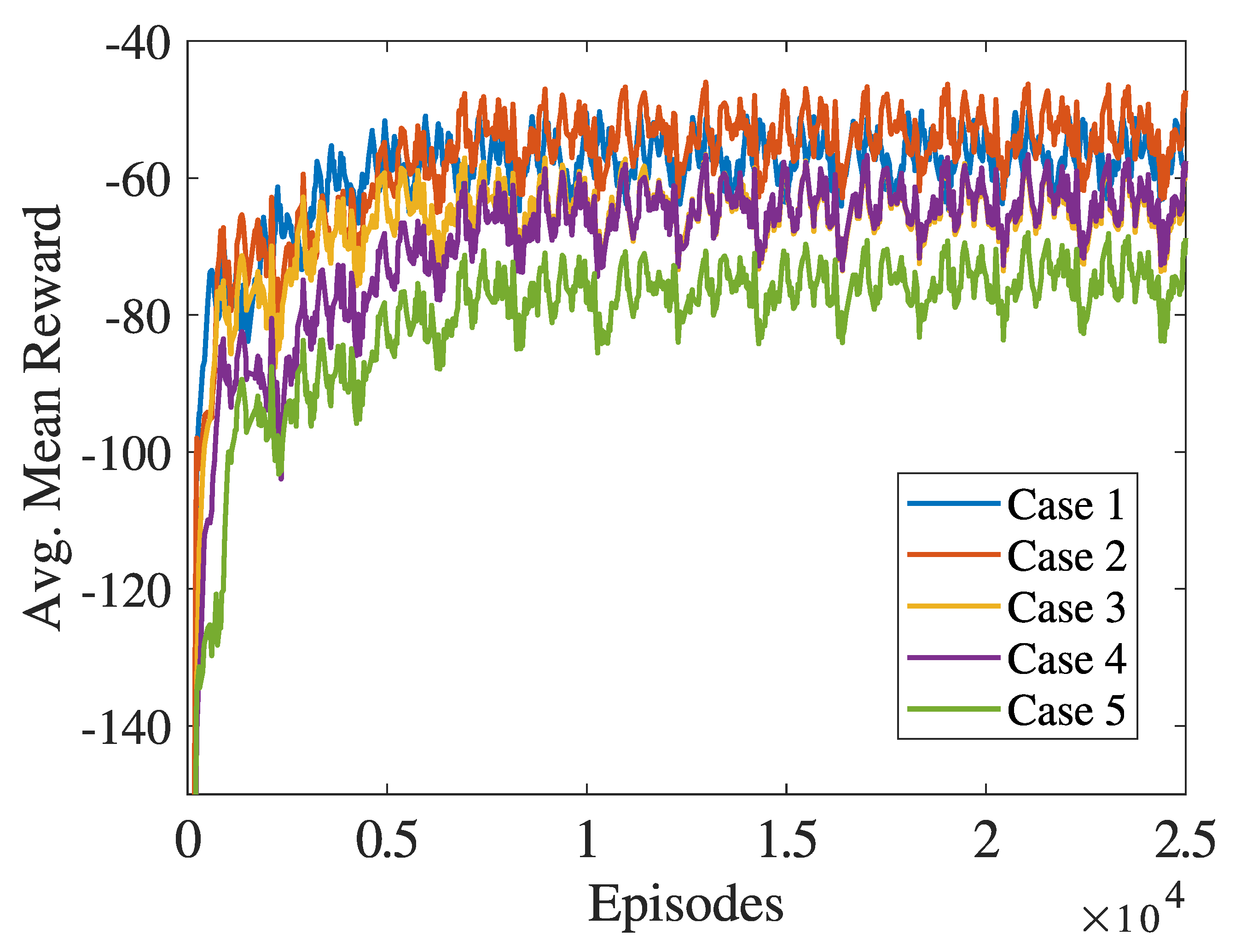
Overall, five different configurations were tested, evaluating various factors including the presence or absence of renewables, the use of a non-polynomial cost function, and the implementation of direct voltage control (otherwise, the voltage was set at 1 p.u. for all generators). As previously mentioned, a load profile obtained with seed 42 and a generation profile obtained from data collected during 2018 were used for the training. Similarly, a load profile obtained with seed 2 and a generation profile obtained from data collected during 2019 were used for the evaluation. To speed up simulation times, only a subset of data was used for training. In case 1, one hour was selected out of every three from the initial 336 h (thus considering 112 h for each month). This specific number of hours was determined empirically and allows a good balance between the accuracy and speed of simulations. In subsequent scenarios, one hour was chosen for every two hours always considering the first 336 h (thus considering 168 h for each month). For all cases, the training process was conducted over 25,000 episodes. For the evaluation, the entire annual profile was taken into account.

To assess the performance of the model four values were considered: the cost comparison in percentage $\kappa$, the accuracy ratio $\eta$, calculated as in (21) [18] and (22) respectively, the simulation time and generation cost are considered.

$${\kappa }_{\%}={\displaystyle \frac{cos{t}_{ref}-cos{t}_{RL}}{cos{t}_{ref}}}·100$$

(21)

$$\eta ={\displaystyle \frac{{\sum }_{h\in H}cos{t}_{ref,h}}{{\sum }_{h\in H}cos{t}_{RL,h}}}\forall h\in H$$

(22)

With $cos{t}_{ref}$ the cost of the reference, $cos{t}_{Rl}$ the total cost obtained using the RL-based controller, and H the total number of hours considered in the simulation.

An overview of all the scenarios is presented in

Table 1. Description of the characteristics in the different case studies and the corresponding cost function. The equations of each cost function are described in Section 3.

	Case 1	Case 2	Case 3	Case 4	Case 5
RES presence	No	Yes	Yes	Yes	Yes
Voltage control	No	No	No	Yes	Yes
Valve point effect	No	No	Yes	No	Yes
Cost function	${\mathrm{CF}}_1$	${\mathrm{CF}}_1$	${\mathrm{CF}}_2$	${\mathrm{CF}}_3$	${\mathrm{CF}}_4$

.

All simulations were conducted using an Intel i7-11800H processor running at 2.30 GHz with 32 GB of RAM. Before presenting the results obtained from the simulations, it is essential to describe the data used for agent training and evaluation. This is crucial as it shows the uniqueness of this b10. Indeed, the models obtained from agent training are tested on real profiles and, therefore, have the potential for online use in real network management. Additionally, a subsection of the chapter is devoted to the description of the neural networks used and the hyperparameter tuning process, given their significance in the learning process.

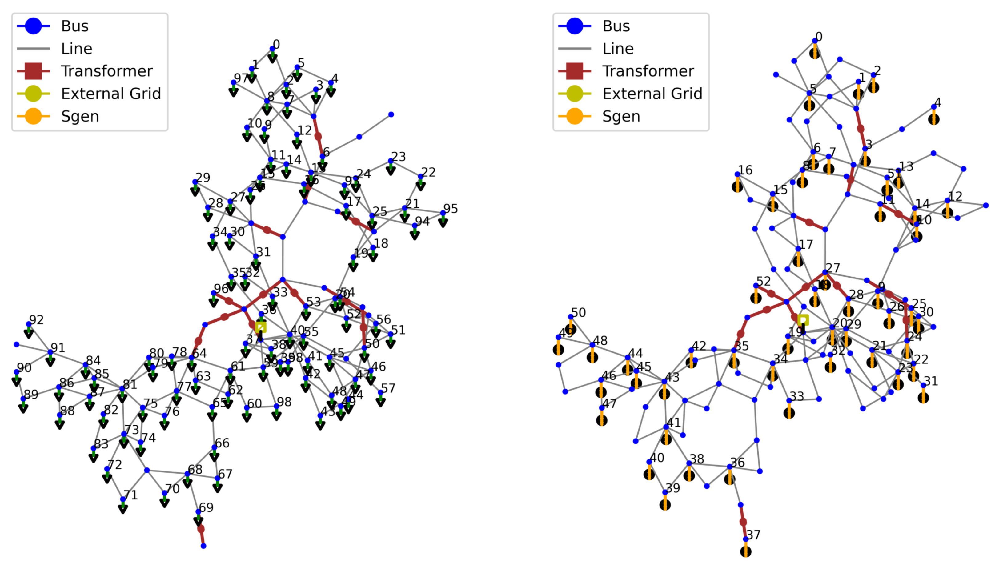
5.1. IEEE 118-Bus System

The IEEE 118-bus test system is a widely used benchmark for power system analysis and research purposes. It represents a simplified model of an actual power system, designed to test and validate various algorithms and methodologies in power system analysis, optimization, and control. The original IEEE 118-bus system contains 19 generators, 35 synchronous condensers, 177 lines, 9 transformers, and 91 loads while the configuration used in this paper is slightly different. It consists of 118 buses, 99 loads, 53 generators, 1 external grid, 173 lines, and 13 transformers operating between voltage levels of 138 - 161 and 345 kV. Overall there are 54 cost functions characterized by the default coefficients. In Figure 3 all the elements characterizing the network, including their indices are represented. The buses position is set using geographical coordinates so it coincides with the real one.

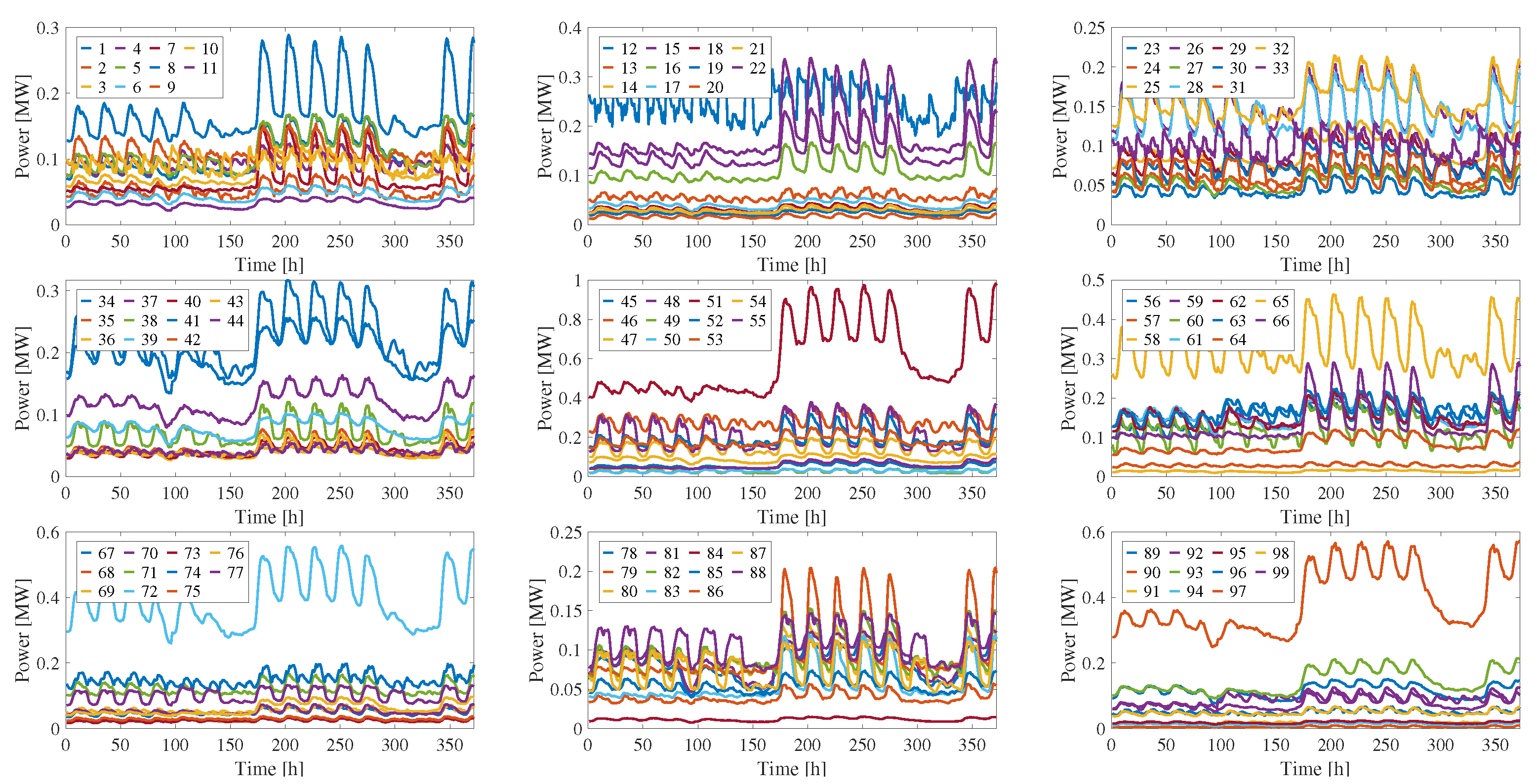
5.2. Loads Profiles

The load profiles used for the training and the evaluation of the agent were extracted from a data collection presented in [29]. It contains a one-year data repository of hourly electrical load profiles from 424 French industrial and tertiary sectors. The dataset contains 18 electricity load profiles derived from hourly consumption time series collected continuously over one year from a total of 55,730 customers. All data was appropriately scaled to ensure compatibility with the network under analysis. Since the test system includes 99 different loads, a corresponding number of distinct load profiles was required. To address this, 99 new profiles were generated through suitable linear combinations of the original 18, allowing the creation of realistic yet differentiated load behaviors for each network load. This process was repeated twice to obtain two distinct sets of data, one for training and one for evaluation. In Figure 4, the 99 load profiles used for training (generated using a seed value of 42) are shown. The profiles used for the evaluation were generated similarly using a different seed value of 2. In both cases, the seed was used to generate multiple load profiles from the existing ones. This was necessary due to the limited availability of only 18 real profiles, whose role was limited to serving as building blocks in the generation of the complete set of 99 distinct profiles required for the simulation.

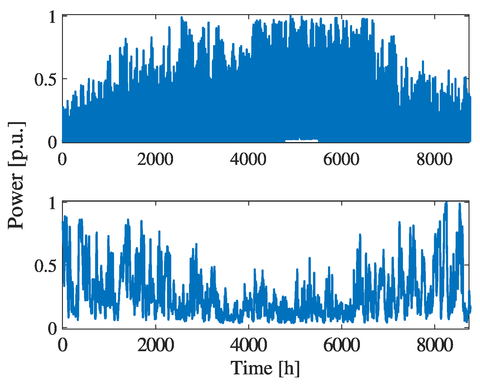
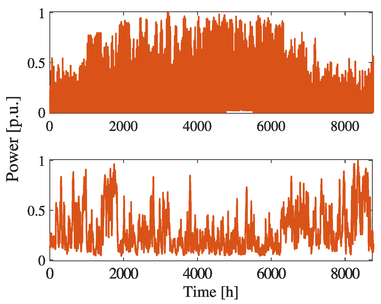
5.3. RES Profiles

To test the algorithm under conditions of uncertainty, renewable energy generators with a peak power of 200 $\mathrm{M}$$\mathrm{W}$ for photovoltaic and a 300 $\mathrm{M}$$\mathrm{W}$ for wind were installed randomly in the network. res generators are modeled as PQ-buses in the PF calculation. The hourly trends of their production profiles were those collected in France during 2018 (for training) and 2019 (for evaluation) and are available on the ENTSO-E website [30]. The profiles are depicted in Figure 5 and Figure 6.

5.4. Neural Network and Hyperparameter Tuning

The TD3 algorithm is characterized by six different neural networks. These have been modeled as simple MLP networks with a number of inputs equal to the number of observations and a number of outputs equal to the number of actions. Case 1 is characterized by 6 hidden layers with (2000, 1000, 1000, 500, 400, 300) neurons. Cases 2 and 3 have 7 hidden layers with (2000, 1000, 1000, 500, 500, 400, 200) since the complexity of the problem has increased. Cases 4 and 5 have 7 hidden layers with (2000, 1000, 1000, 500, 500, 400, 300) due to the higher number of actions to be taken. The number of nodes of the NN, as well as other hyperparameters of the neural network, were obtained using an optimization algorithm based on Optuna [31]. Practically, various parameter configurations were tested by training the agent with a fixed network configuration. The configuration that yielded the best results in terms of reward was saved and used for all case studies. The parameters are summarized in

Table 2. Hyperparameters.

Parameters	Value
$\gamma$ = discount factor	$0.9999$
learning rate = adam opt. update rate	$0.000495$
batch size = minibatch size for gradient update	256
buffer size = size of replay buffer	$\mathrm{100,000}$
$\tau$ = soft update coeff.	$0.005$
train freq = model update rate	4
noise type = random action noise	normal
noise std = noise standard deviation	$0.174$

.

All the other hyperparameters are kept at default values.

5.4.1. Case 1

In this initial case, the OPF was executed for the original network without RES. The cost function considered is polynomial, using the default network coefficients $c_0$, $c_1$, and $c_2$ for each generator. The Pandapower interior-point method (IPM) solver was employed as a comparative method.

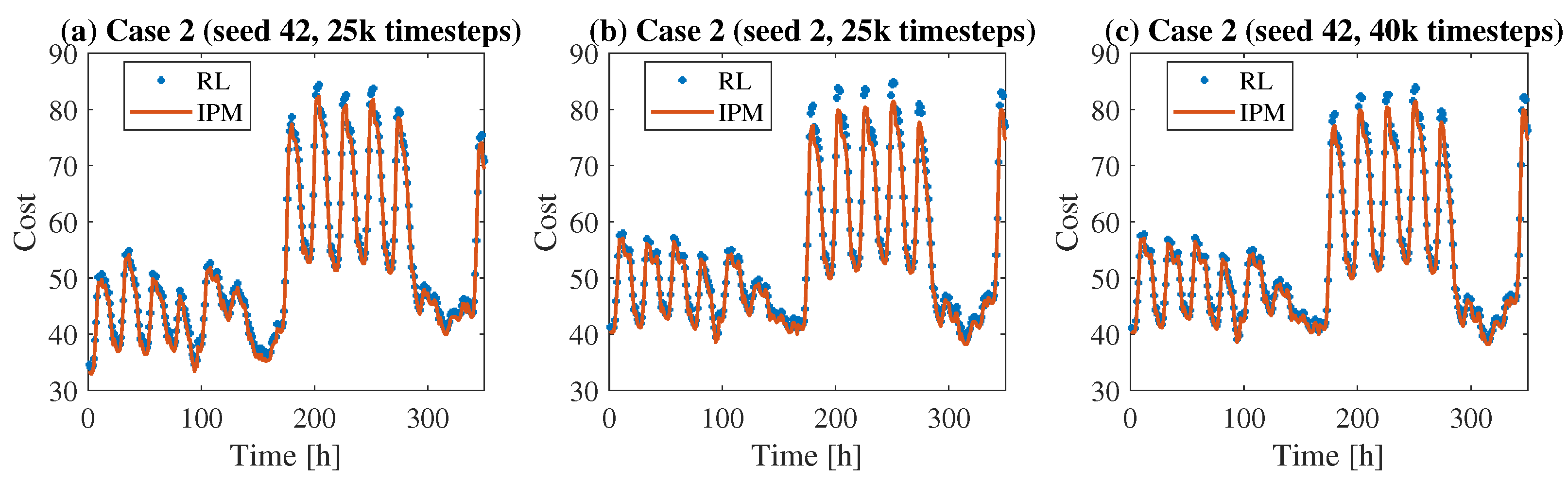
5.4.2. Case 2

The second case is similar to the previous one, with the addition of some non-dispatchable renewable generators, such as solar and wind. The cost of these generators is set to zero, assuming that the network under investigation prioritizes the dispatch of RESs. Therefore, it is assumed that at each hour, all power generated by non-programmable sources is absorbed by the loads. What can be modified is solely the production profile of the other 53 programmable generators. Since the cost function remains unchanged compared to case 1, the IPM solver is still used as a comparative method. In Figure 7 the cost values obtained with the algorithms are shown. In Figure 7c it is evident how the number of timesteps used for the training impacts the accuracy of the RL algorithm.

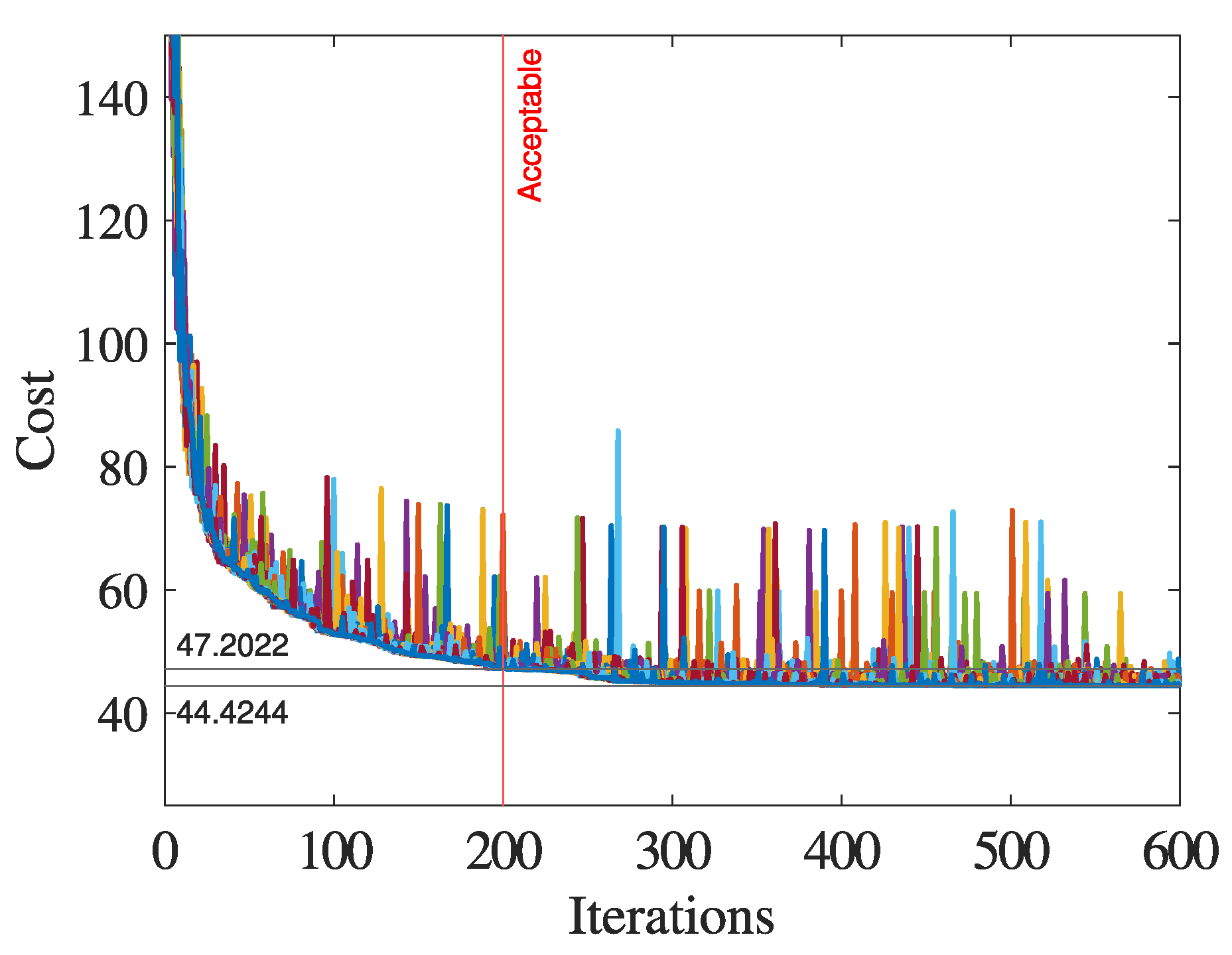
5.4.3. Case 3

This case takes into account the valve point effect in generators. Therefore, in this scenario, the comparative method used is the genetic algorithm (GA). Initially, particle swarm optimization (PSO) was used as a comparison method. This choice was made because such algorithms typically guarantee convergence for very large action spaces within relatively short time-frames. However, given the size of the network, the PSO in our tests was never able to achieve cost values comparable to those obtained with RL. For this reason, the slower but more robust GA-based method was used. In Figure 8, it is evident that taking the first set of loads (hour 1) as an example, the algorithm can reach the minimum point in about 600 iterations. The time required for this simulation is approximately 30 min. However, a satisfactory result can be achieved in just 200 iterations, corresponding to about 8 min of simulation. Independently on the number of iterations, the population size was set to 50. Even considering only 200 iterations, the total simulation time exceeds two months. Therefore, we decided to simulate only the first 20 h. This is a time interval sufficient to allow a comparison with the RL. In all simulations where the valve point effect was considered $c_3$ and $c_4$ were set to 200 and 0.2 respectively.

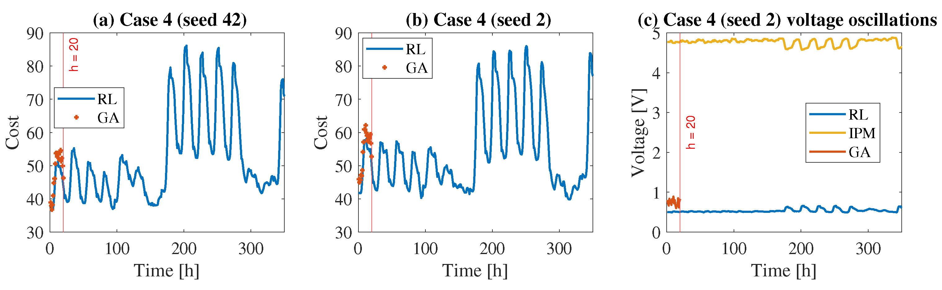
5.4.4. Case 4

This scenario represents the implementation of soft voltage constraints, as described by the cost function ${\mathrm{CF}}_3$. In this cost function, the primary goal is to minimize voltage fluctuations at each bus, ensuring they stay close to their nominal values (set to 1 p.u.), while also minimizing the overall cost function. The soft constraint introduces a penalty in the cost function to discourage the generation profiles that cause significant voltage deviations from the nominal value (1 p.u.) at the network buses. The GA is used as the method of comparison. The results concerning the first 350 h are summarized in Figure 9 (GA time refers only to the first 20 h because due the computational time the entire simulation would last more than 2 months). More specifically, Figure 9c highlights the sum of voltage deviations from the nominal value across all nodes of the network, computed on an hourly basis. This sum represent the portion of the cost function ${\mathrm{CF}}_3$ relate to the soft constraints, and we use it to analyzed the influence of the minimization of this contribution in the three algorithms compared. It is observed that the inclusion of voltage constaints results in a reduction of about 1/5 compared to the case without voltage control(IPM), and nearly a 20% reduction when compared to the results obtained using the ga with voltage control.

5.4.5. Case 5

Here, the cost function ${\mathrm{CF}}_4$ is minimized, thereby taking into account all the complexities of the problem. The figure illustrates the annual production profile from programmable sources, considering the valve point effect, voltage control, and the presence of renewable energy sources.

All the numerical results and the training curves are summarized in Figure 10 and

Table 3. Summary table comparing RL, IPM, and GA for the different use cases. The table reports the simulation times along with key metrics for evaluating the accuracy of the solutions.

	Seed	Case 1	Case 2	Case 3	Case 4	Case 5
Training time [hh:mm:ss]	42	00:43:38	00:41:38	00:42:02	00:48:40	00:52:45
	2	-	-	-	-	-
Testing time [hh:mm:ss]	42	00:14:02	00:14:19	00:14:29	00:15:16	00:15:45
	2	00:14:18	00:14:45	00:15:16	00:15:11	00:15:41
IPM time [hh:mm:ss]	42	01:21:01	01:23:36	-	-	-
	2	01:21:06	01:23:48	-	-	-
GA time [hh:mm:ss]	42	-	-	02:41:03	02:42:22	03:00:56
	2	-	-	02:43:47	02:46:41	02:44:09
Min ${\kappa }_{\%}$	42	−3.7354	−4.3765	1.7544	0.6540	−0.1955
	2	−4.8428	−5.3971	1.6859	3.1074	3.9557
Max ${\kappa }_{\%}$	42	−1.1494	−1.1054	7.2116	11.1058	8.7405
	2	−1.3537	−1.0731	5.3945	11.3327	7.5161
Average ${\kappa }_{\%}$	42	−2.2387	−1.9352	3.9119	6.4399	4.7417
	2	−1.9895	−1.9680	3.3101	6.6094	5.4086
Accuracy $\eta$	42	0.9791	0.9820	1.0405	1.0703	1.0518
	2	0.9802	0.9805	1.0337	1.0695	1.0575

Notes: GA time refers only to the first 20 h (the entire simulation would last more than 2 months).

. The percentage of times the OPF is solved without violating constraints is $100\%$ in all cases.

5.5. Practical Applicability to Real-World Power Systems

The presented RL-based OPF framework has promising applicability in real-world power system operations, particularly in contexts requiring fast, adaptive decision-making under uncertainty. A key advantage of the proposed approach is its ability to generalize beyond the specific conditions seen during training. The trained RL agent was evaluated on previously unseen scenarios, featuring different load and generation profiles, including the presence of non-dispatchable RESs, valve-point effects, and voltage regulation objectives. This highlights the method’s robustness and adaptability to dynamic and realistic operating conditions that are often difficult to model explicitly.

Once trained, the policy can be deployed within energy management systems or embedded into distributed controllers to provide near-optimal decisions in real time, avoiding the computational burden of solving OPF from scratch at each step. Moreover, the proposed approach has shown the capability to respect key operational constraints, such as generator limits and voltage deviations, through reward shaping and interaction with the simulated environment. This makes it suitable for deployment in both transmission and distribution networks with high variability and DER integration. The RL-based solution can also be integrated into hierarchical or hybrid control architectures, where its outputs are validated or refined by conventional solvers to ensure operational security and regulatory compliance. The ability to react to novel conditions with fast inference times suggests its suitability for real-time or near-real-time applications, offering a scalable alternative to traditional optimization methods in future power system operation frameworks.

6. Conclusions

This paper proposes a novel methodology based on RL to solve the OPF problem. The approach leverages theTD3 algorithm, enabling the system to reach optimal operating conditions while accounting for complex factors such as the valve-point effect of gas-fired generators, the integration of non-dispatchable RESs, and voltage regulation at the bus level. The method was validated on the IEEE 118-bus system using five distinct case studies. To enhance realism, both the RES generation and load consumption profiles were derived from actual data.

The results demonstrate that the algorithm is both robust and reliable, consistently converging to the optimal solution more quickly than traditional techniques such as the IPM and GA. In the case under study, the RL model achieves a comparable level of accuracy, with only a slight reduction (about 1–2%) compared to ipm, while offering a substantial reduction in computation time of around 30%. Although metaheuristic methods like ga may yield competitive solutions, their computation times become impractically long as network complexity grows, making the RL-based approach a more scalable and efficient alternative. Furthermore, unlike traditional methods, the RL model is inherently suited to handle the uncertainty associated with RESs, whose production is often highly variable and difficult to forecast.

Future research will focus on developing algorithms that initialize the parameters of NN based on historical data, thereby reducing the time required for simulations and increasing the accuracy of the outputs. Additionally, the development of a multi-agent RL model is planned, enabling optimal decentralized management of networks with high RES penetration. In this model, each agent would manage a portion of the electric network and share information with other nodes through a dedicated buffer. This type of logic would allow for managing sudden changes in network topology, for example, due to faults, and planning the provision of ancillary or network support services.