Disturbance Rejection and Uncertainty Analysis in Wind Turbines Using Model Predictive Control

Abstract

For effective wind turbine operations, it is essential to maintain the power limit and reduce the stress on the drive train in the presence of disturbance and uncertain conditions. In our work, we propose a Model Predictive Control (MPC) framework with quadratic cost functions, incorporating control input and state constraints to mitigate the challenge of disturbance rejection and uncertainty analysis for the wind turbine operation. We have tailored the algorithm to the practical parameters of the National Renewable Energy Laboratory’s (NREL) Controls Advanced Research Turbine (CART) model. We illustrate the impact of wind disturbances on achieving the optimal control law and evaluate the performance of integral MPC in disturbance rejection for the wind turbine operation, comparing it with the constrained optimal control law outcomes. The simulation results also show the efficacy of integral MPC for the uncertainty in the initial conditions of the wind turbines. This is shown by the propagation of the first two moments, i.e., mean and variance, for the states of the wind turbine. Further, we obtained the control law and mean–variance propagation for the variation in disturbance intensity. The overall results prove the efficacy of using the MPC framework for uncertainty analysis and disturbance rejection to obtain optimal operation in wind turbines.

1. Introduction

Wind power is a highly promising sustainable renewable energy source, poised to make a substantial contribution to global energy needs [1]. According to the International Energy Agency (IEA), in 2022, wind power generation surged by 265 TWh (14% increase), surpassing 2100 TWh [2]. However, this growth, second only to solar PV, must still catch up to the trajectory needed to achieve the goal of Net Zero Emissions by 2050. The 2022 Inflation Reduction Act in the United States of America allocated significant funding for wind power [3] to various places. As a result, the East Coast of the United States of America launched its first large-scale offshore wind project, which is expected to have 62 operational turbines in the near future. The variable power output of wind turbines is heavily influenced by environmental disturbances such as wind speed, wind direction, and turbulence [4]. Aerodynamic disturbances [5] present a major challenge in different forms, such as turbulent wind inflow, wind shear, and gusts. These challenges have the potential to lead to unsteady aerodynamic loading on the blades of the wind turbine. These fluctuations reduce the energy conversion efficiency of the wind turbine system and induce fatigue loads that can compromise the structural health of the wind turbine components over time. Another challenge is structural disturbances [6] such as tower shadow effects, blade tower interactions, and dynamic coupling between different wind turbine components, further complicating the behavior of the whole system. Addressing disturbances is crucial to enhancing the efficiency and longevity of wind turbines. The challenge lies in minimizing the fatigue caused by these disturbances while maximizing the power output of the whole system [7,8]. Larger wind turbines, designed to produce more power, are particularly susceptible to significant fatigue, which can shorten their operational lifespan. Therefore, effective disturbance rejection not only improves the wind turbine efficiency but also extends the lifetime of components, leading to better cost benefits of operating the wind turbine. This focus on mitigating environmental disturbances encourages researchers to develop methods that optimize the power output of wind turbines without compromising their durability.

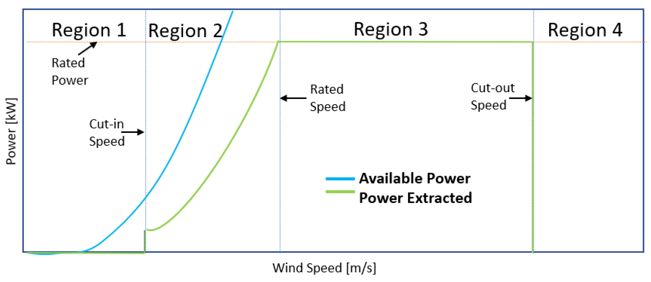
Wind turbines typically operate in four distinct regions, each with specific control objectives determined by the wind speed and power, as illustrated in Figure 1. We focus on the operation of wind turbine in Region 3, the full load region, where the turbine generates rated power at wind speeds exceeding the rated speed but below the cut-out speed. In this region, the primary control objective is maintaining power output at the rated level while ensuring the turbine’s safe operation.

In a wind turbine, the aerodynamic torque is governed by the pitch angle and blade position, which are regulated to achieve the desired power output. To enhance wind turbine performance and mitigate structural fatigue due to disturbance, pitch angle control methods have been explored in [8,9]. Traditionally, Proportional Integral Derivative (PID) controllers have been used for wind turbine control [10], with controller gain adjusted for different requirements such as power output and drive train twist. However, the effectiveness of these controllers can vary depending on the operational regions, with some being more suited to specific regions and others transitioning between regions [11]. Various other methods have been explored to tackle this challenge, including adaptive controllers [12], feedback linearization techniques [13], robust control [14], a nonlinear controller [15], and methods based on Maximum Power Point Tracking (MPPT) [16] to enhance the turbine efficiency.

Since the late 2000s, methods employing optimization techniques in controlling wind turbines have been explored [17]. As a result, various methodologies utilize MPC formulations to enhance the wind turbine operation [18,19,20]. Using various practical constraints on parameters of the system, these methods achieve the control objectives like enhancing power generation or mitigating tower loads [21] in the wind turbine operation. MPC proves highly beneficial for wind turbine control because it manages multivariable constraints on both system inputs and states. It also provides predictive functionalities, allowing for optimized control inputs by considering future predictions for disturbance rejection [22,23]. However, the MPC approach must be appropriately explored for effective disturbance rejection problems in wind turbine operations, which is the main purpose of our work.

In this work, we have formulated an optimal control framework using a linear MPC-based approach for wind turbine operation in Region 3, focusing on designing a pitch angle controller for disturbance rejection and uncertain initial conditions. We used practical parameters from the NREL’s Controls Advanced Research Turbine (CART) model and defined the optimal control problem with a quadratic cost function involving state variables and control inputs. We have considered the constraints on the state and input of the wind turbine system and compared the results with those of unconstrained MPC to analyze the effectiveness of the MPC framework.

Recognizing that the operation of wind turbines is continuously exposed to disturbances, we previously discussed the MPC framework for disturbance rejection in [24]. Our findings showed that MPC performs satisfactorily even in the presence of disturbances. In this work, we have utilized integral MPC for disturbance rejection to address the losses due to steady-state error. Although integral MPC may slow down the system, it significantly reduces the steady-state error, enhancing overall performance in managing disturbances of the system. We have also shown the integral MPC results for the wind turbine’s varying initial conditions and the change in disturbance intensity to analyze the effectiveness of MPC for uncertainty analysis. In our work, we have utilized a deterministic approach for computationally efficient and systematic exploration of how disturbance inputs affect a wind turbine’s dynamic response. This can be helpful in isolating specific uncertainty sources and their impact on system behavior, enhancing reproducibility and clarity in assessing stability. The mean and variance propagation plot provides the uncertainty analysis for the initial conditions by analyzing the expected value and the corresponding dispersion of states of wind turbines about the mean at future times. The results strengthen the efficacy of the proposed MPC controller design in the case of uncertainty in initial conditions and change in disturbance intensity. It facilitates the scope to evaluate and improve our control action strategy, providing wind turbines with more efficient and reliable operation.

The structure of the paper is outlined as follows. Section 2 presents the formulation of wind turbine dynamics. In Section 3, we detail the optimal control formulation for disturbance rejection and provide the preliminaries for the statistical analysis. We provide the MPC problem formulation for the wind turbine in Section 4. Section 5 showcases the simulation results. Finally, Section 6 summarizes the entire paper and highlights potential directions for future research.

2. Dynamics of the Wind Turbine

In this section, we will discuss the dynamics of the wind turbine model used in our work. We will first discuss the details of the nonlinear equations of the system, which are further linearized around the operating point of the wind turbine system.

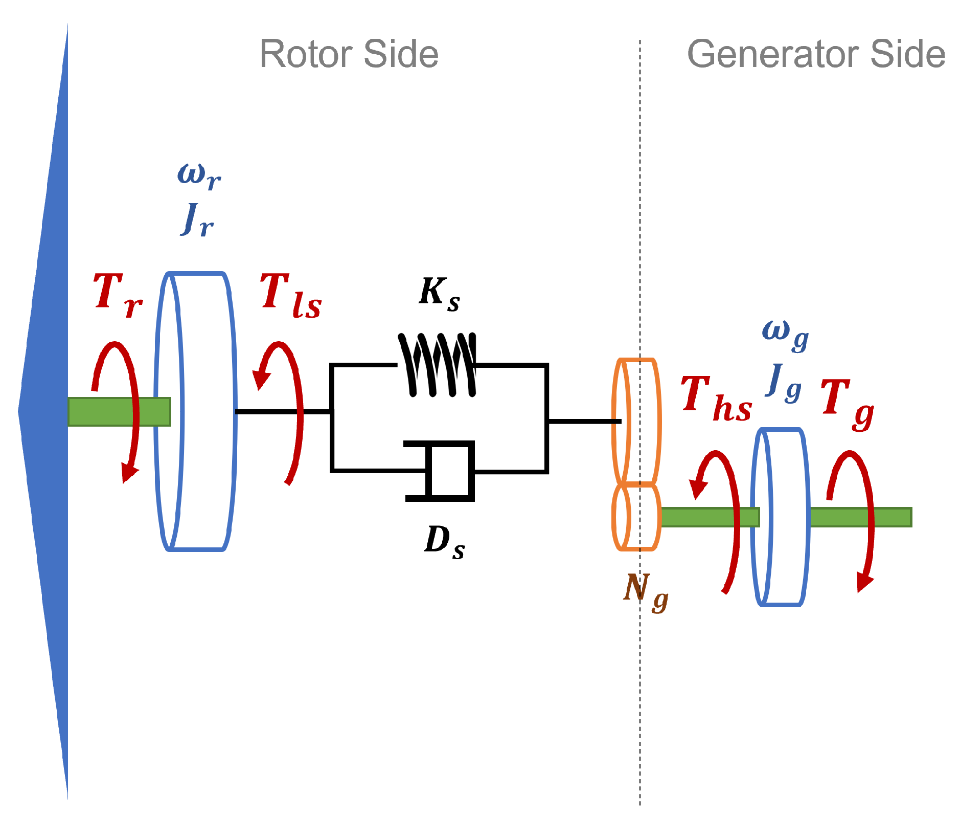
The rotor of a wind turbine includes blades and a hub, which convert wind energy into mechanical energy. In high wind speed conditions, the turbine’s control system adjusts the pitch angle of the blades to maintain a consistent power output from the system. The drive train of the wind turbine transmission can be simplified using a two-mass model, as illustrated in Figure 2. It is assumed that the gearbox operates with perfect mechanical efficiency.

The wind turbine model’s nonlinear generalized dynamics are described by the following mathematical equation:

$$\begin{array}{c}\hfill \dot{\mathbf{z}}=\mathbf{F}\left(\mathbf{z}\right)+\mathbf{B}u.\end{array}$$

(1)

Here, $\mathbf{F}\left(\mathbf{z}\right)$ is given as below and whose variables are discussed ahead:

$$\begin{array}{cc}\hfill \mathbf{F}\left(\mathbf{z}\right)& =\left[\begin{array}{c}{f}_1\\ f_2\\ f_3\\ f_4\end{array}\right]=\left[\begin{array}{c}{\displaystyle \frac{P_r(z_1,z_4,V)}{z_1{J}_r}}-{\displaystyle \frac{z_1{D}_s}{J_r}}+{\displaystyle \frac{z_2{D}_s}{J_r}}-{\displaystyle \frac{z_3{K}_s}{J_r}}\\ {\displaystyle \frac{z_1{D}_s}{N_g{J}_g}}-{\displaystyle \frac{z_2{D}_s}{N_g^2{J}_g}}+{\displaystyle \frac{z_3{K}_s}{N_g{J}_g}}-{\displaystyle \frac{T_g}{J_g}}\\ z_1-{\displaystyle \frac{z_2}{N_g}}\\ -{\displaystyle \frac{1}{{\tau }_{\beta }}}{z}_4\end{array}\right].\hfill \end{array}$$

(2)

The control input matrix for the wind turbine is denoted by $\mathbf{B}={\left[\begin{array}{cccc}0& 0& 0& {\displaystyle \frac{1}{{\tau }_{\beta }}}\end{array}\right]}^T$, with the state vector $\mathbf{z}={\left[\begin{array}{cccc}{\omega }_r& {\omega }_g& \delta & \beta \end{array}\right]}^T$ and control input $u={\beta }_r$. Using these variables, we can write Equation (1) as:

$$\begin{array}{c}\hfill \dot{\mathbf{z}}=\left[\begin{array}{c}{\displaystyle \frac{P_r(z_1,z_4,V)}{z_1{J}_r}}-{\displaystyle \frac{z_1{D}_s}{J_r}}+{\displaystyle \frac{z_2{D}_s}{J_r}}-{\displaystyle \frac{z_3{K}_s}{J_r}}\\ {\displaystyle \frac{z_1{D}_s}{N_g{J}_g}}-{\displaystyle \frac{z_2{D}_s}{N_g^2{J}_g}}+{\displaystyle \frac{z_3{K}_s}{N_g{J}_g}}-{\displaystyle \frac{T_g}{J_g}}\\ z_1-{\displaystyle \frac{z_2}{N_g}}\\ -{\displaystyle \frac{1}{{\tau }_{\beta }}}{z}_4\end{array}\right]+\left[\begin{array}{c}0\\ 0\\ 0\\ {\displaystyle \frac{1}{{\tau }_{\beta }}}\end{array}\right]{\beta }_r.\end{array}$$

(3)

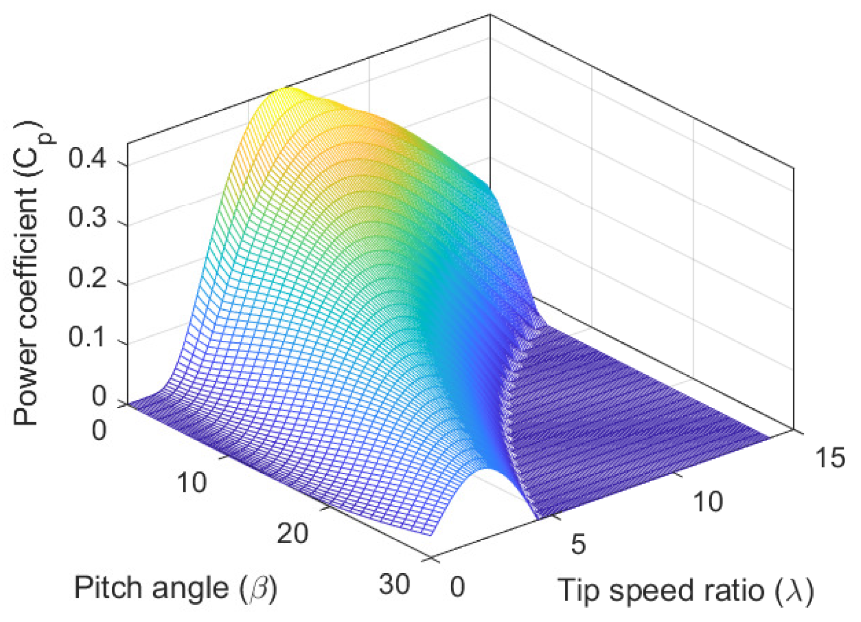
The mechanical power ($P_r$) captured by the wind turbine is given by $P_r={\displaystyle \frac{1}{2}}\pi \rho R^2{V}^3{C}_p(z_1,z_4,V)$. The nonlinear power coefficient ($C_p$), which depends on the pitch angle ($\beta$) and tip-speed ratio ($\lambda$), is shown in Figure 3, and the expression is given as:

$$\begin{array}{cc}\hfill C_p& =0.22(116{\lambda }_t-0.4z_4-5)e^{-12.5{\lambda }_t},\hfill \end{array}$$

(4)

$$\begin{array}{cc}\hfill {\lambda }_t& ={\displaystyle \frac{1}{\lambda +0.08\beta }}-{\displaystyle \frac{0.035}{{\beta }^3+1}},\lambda ={\displaystyle \frac{{\omega }_{r}R}{V}}.\hfill \end{array}$$

(5)

Other parameters of the wind turbine dynamical equation are given in

Table 1. Parameters of the model.

Parameter	Definition
${\omega }_r,{\omega }_g$	Rotor speed, Generator speed
$\delta ,\beta$	Twist angle, Pitch angle
${\tau }_{\beta }$	Time constant of pitch actuator
${\beta }_r$,$T_g$	Pitch angle control, Generator torque
$J_r,J_g$	Rotor inertia, Generator inertia
$N_g,\lambda$	Gear ratio, Tip-speed ratio
$D_s,K_s$	Drive-train damping, Spring constant
R, $\rho$, V	Rotor radius, Air density, Wind speed
$C_p$	Power conversion coefficient

.

We linearize the nonlinear dynamics of the wind turbine model given in (3) around an operating point $\tilde{\mathbf{z}}={\left[\begin{array}{cccc}2.14& 188.4& 0& 25\end{array}\right]}^T$ to obtain the system matrix $\mathbf{A}$ for the linearized model of wind turbine. The elements of $\mathbf{A}$ are computed as the partial derivatives of $\mathbf{F}$ with respect to $\mathbf{z}$, evaluated at $\tilde{\mathbf{z}}$ with values as follows:

$$\begin{array}{cc}\hfill {\displaystyle \frac{\partial f_1\left(\mathbf{z}\right)}{\partial z_1}}& =-{\displaystyle \frac{D_s}{J_r}}-{\displaystyle \frac{1}{J_r{z}_1}}[{\displaystyle \frac{P_r}{z_1}}+0.11\pi \rho R^3{V}^2{\displaystyle \frac{178.5-1450{\lambda }_t+5z_4}{{(\lambda +0.08z_4)}^2}}{e}^{-12.5{\lambda }_t}],\hfill \\ \hfill {\displaystyle \frac{\partial f_1\left(\mathbf{z}\right)}{\partial z_2}}& ={\displaystyle \frac{D_s}{N_g{J}_r}},\hfill \\ \hfill {\displaystyle \frac{\partial f_1\left(\mathbf{z}\right)}{\partial z_3}}& =-{\displaystyle \frac{K_s}{J_r}},\hfill \\ \hfill {\displaystyle \frac{\partial f_1\left(\mathbf{z}\right)}{\partial z_4}}& ={\displaystyle \frac{0.11\pi \rho R^2{V}^3}{z_1{J}_r}}\{(178.5-1450{\lambda }_t+5z_4)[{\displaystyle \frac{-0.08}{{(\lambda +0.08z_4)}^2}}+{\displaystyle \frac{0.105z_4^2}{{(z_4^3+1)}^2}}]-0.4\}{e}^{-12.5{\lambda }_t},\hfill \\ \hfill {\displaystyle \frac{\partial f_2\left(\mathbf{z}\right)}{\partial z_1}}& ={\displaystyle \frac{D_s}{N_g{J}_g}},\hfill \\ \hfill {\displaystyle \frac{\partial f_2\left(\mathbf{z}\right)}{\partial z_2}}& =-{\displaystyle \frac{D_s}{N_g^2{J}_g}},\hfill \\ \hfill {\displaystyle \frac{\partial f_2\left(\mathbf{z}\right)}{\partial z_3}}& ={\displaystyle \frac{K_s}{N_g{J}_g}},\hfill \\ \hfill {\displaystyle \frac{\partial f_2\left(\mathbf{z}\right)}{\partial z_4}}& =0,\hfill \\ \hfill {\displaystyle \frac{\partial f_3\left(\mathbf{z}\right)}{\partial z_1}}& =1,\hfill \\ \hfill {\displaystyle \frac{\partial f_3\left(\mathbf{z}\right)}{\partial z_2}}& =-{\displaystyle \frac{1}{N_g}},\hfill \\ \hfill {\displaystyle \frac{\partial f_3\left(\mathbf{z}\right)}{\partial z_3}}& =0,\hfill \\ \hfill {\displaystyle \frac{\partial f_3\left(\mathbf{z}\right)}{\partial z_4}}& =0,\hfill \\ \hfill {\displaystyle \frac{\partial f_4\left(\mathbf{z}\right)}{\partial z_1}}& ={\displaystyle \frac{\partial f_4\left(\mathbf{z}\right)}{\partial z_2}}={\displaystyle \frac{\partial f_4\left(\mathbf{z}\right)}{\partial z_3}}=0,{\displaystyle \frac{\partial f_4\left(\mathbf{z}\right)}{\partial z_4}}=-{\displaystyle \frac{1}{{\tau }_{\beta }}}.\hfill \end{array}$$

Our work uses the linearized state-space representation of the wind turbine dynamics as $\dot{\mathbf{z}}=\mathbf{A}\mathbf{z}+\mathbf{B}u$. For the simulation results in MATLAB, we adopt discrete-time dynamics with a zero-order hold on inputs. Next, we will discuss the theory of constructing the MPC formulation aimed at disturbance rejection and a quick overview of uncertainty analysis.

3. MPC Problem Formulation for Disturbance Rejection

In our work, we propose an MPC framework for the wind turbine system’s disturbance rejection and uncertainty analysis. In this section, we will discuss the various MPC frameworks that are utilized in our work. These are based on the linearized state-space representation of the wind turbine dynamics obtained in the previous section.

3.1. MPC Framework for Constraints

MPC is a robust tool for solving optimal control design problems, providing significant advantages over traditional PID controllers, such as handling constraints and rejecting disturbances. This section presents a formal methodology for applying MPC to determine the optimal control law for disturbance rejection for a discrete-time linear dynamical system. We consider the dynamics of the form:

$$\begin{array}{c}\hfill \mathbf{z}(k+1)=\mathbf{A}\mathbf{z}\left(k\right)+\mathbf{B}\mathbf{u}\left(k\right),\mathbf{y}\left(k\right)=\mathbf{C}\mathbf{z}\left(k\right),\end{array}$$

(6)

where $\mathbf{z}\in {\mathbb{R}}^n$ represents the state variables, $\mathbf{u}\in {\mathbb{R}}^m$ is the control input, and $\mathbf{y}\left(k\right)$ denotes the measured outputs.

Assumption 1.

A1. 

The pair $(\mathbf{A},\mathbf{B})$ is stabilizable, and the pair $(\mathbf{A},\mathbf{C})$ is detectable. The dynamical systems focus on full-state feedback.

A2. 

Consider constant constraints across the prediction horizon. Therefore, at each time step, we have constant matrices given as ${\mathbf{M}}_i=\mathbf{M}$, ${\mathbf{E}}_i=\mathbf{E}$, and ${\mathbf{b}}_i=\mathbf{b}$.

For now, we assume the dynamics are free from disturbances, delays, model errors, and noise. Our goal is to solve the finite horizon optimal control problem by minimizing the cost function $\mathcal{J}(\mathbf{z}\left(0\right),\mathbf{u})={\mathbf{z}}^{\top }\left(N\right)\mathbf{P}\mathbf{z}\left(N\right)+{\sum }_{i=0}^{N-1}\{\mathbf{z}{\left(i\right)}^{\top }\mathbf{Q}\mathbf{z}\left(i\right)+\mathbf{u}{\left(i\right)}^{\top }\mathbf{R}\mathbf{u}\left(i\right)\}$, where, $\mathbf{Q}⪰\mathbf{0}$, $\mathbf{P}⪰\mathbf{0}, \mathbf{R}\succ \mathbf{0}$, $\mathbf{u}=\left[\mathbf{u}\right(0),\dots ,\mathbf{u}(N-1\left)\right]$, and N is the prediction horizon. The control horizon is often chosen to be shorter than the prediction horizon. In such cases, the remaining control inputs are either held constant or set to zero. However, in our work, we set the control horizon equal to the prediction horizon. By utilizing the recursive relation of the state equation, we can express the following for Equation (6):

$$\begin{array}{cc}\hfill \left[\begin{array}{c}\mathbf{z}\left(1\right)\\ \mathbf{z}\left(2\right)\\ ⋮\\ \mathbf{z}\left(N\right)\end{array}\right]& =\left[\begin{array}{c}\mathbf{A}\\ {\mathbf{A}}^2\\ ⋮\\ {\mathbf{A}}^N\end{array}\right]\mathbf{z}\left(0\right)+\left[\begin{array}{cccc}\mathbf{B}& 0& \dots & 0\\ \mathbf{A}\mathbf{B}& \mathbf{B}& \dots & 0\\ ⋮& ⋮& \dots & \\ {\mathbf{A}}^{N-1}\mathbf{B}& {\mathbf{A}}^{N-2}\mathbf{B}& \dots & \mathbf{B}\end{array}\right]\left[\begin{array}{c}\mathbf{u}\left(0\right)\\ \mathbf{u}\left(1\right)\\ ⋮\\ \mathbf{u}(N-1)\end{array}\right].\hfill \end{array}$$

(7)

The above dynamic model using the stack variables is given as:

$$\begin{array}{c}\hfill \mathbf{Z}=\Phi \mathbf{z}+\Gamma \mathbf{U}.\end{array}$$

(8)

Similarly, the cost function by stacking the variables from above is given as $\mathcal{J}(\mathbf{z}\left(0\right),\mathbf{U})={\mathbf{z}}^{\top }\left(N\right)\mathbf{P}\mathbf{z}\left(N\right)+{\sum }_{i=0}^{N-1}[{\mathbf{z}}^{\top }\left(i\right)\mathbf{Q}\left(i\right)\mathbf{z}\left(i\right)+{\mathbf{u}}^{\top }\left(i\right)\mathbf{R}\left(i\right)\mathbf{u}\left(i\right)]$. The matrix form for the cost function is given as:

$$\begin{array}{cc}\hfill \mathcal{J}\left(\mathbf{z}\right(0),\mathbf{U})& ={\mathbf{z}}^{\top }\left(0\right)\mathbf{Q}\left(0\right)\mathbf{z}\left(0\right)+{\left[\begin{array}{c}\mathbf{z}\left(1\right)\\ \mathbf{z}\left(2\right)\\ ⋮\\ \mathbf{z}\left(N\right)\end{array}\right]}^{\top }\left[\begin{array}{cccc}\mathbf{Q}\left(1\right)& 0& \dots & 0\\ ⋮& \mathbf{Q}\left(2\right)& ⋮& 0\\ & & \ddots & \\ 0& 0& \dots & \mathbf{P}\end{array}\right]\left[\begin{array}{c}\mathbf{z}\left(1\right)\\ \mathbf{z}\left(2\right)\\ ⋮\\ \mathbf{z}\left(N\right)\end{array}\right]+\hfill \\ \hfill & {\left[\begin{array}{c}\mathbf{u}\left(0\right)\\ \mathbf{u}\left(1\right)\\ ⋮\\ \mathbf{u}(N-1)\end{array}\right]}^{\top }\left[\begin{array}{cccc}\mathbf{R}\left(0\right)& 0& \dots & 0\\ 0& \mathbf{R}\left(2\right)& \dots & 0\\ ⋮& ⋮& \ddots & ⋮\\ 0& \dots & \dots & \mathbf{R}(N-1)\end{array}\right]\left[\begin{array}{c}\mathbf{u}\left(0\right)\\ \mathbf{u}\left(1\right)\\ ⋮\\ \mathbf{u}(N-1)\end{array}\right].\hfill \end{array}$$

(9)

We can also write the compact form as $\mathcal{J}(\mathbf{z},\mathbf{U})={\mathbf{z}}^{\top }\mathbf{Q}\mathbf{z}+{\mathbf{Z}}^{\top }\Omega \mathbf{Z}+{\mathbf{U}}^{\top }\Psi \mathbf{U}$. Here, $\mathbf{z}=\mathbf{z}\left(0\right)$. Following from $\mathbf{Q}\left(i\right)⪰\mathbf{0}$, and $\mathbf{P}⪰\mathbf{0}$, we obtain $\Omega ⪰\mathbf{0}$. Similarly, from $\mathbf{R}\left(i\right)\succ \mathbf{0}$, we obtain $\Psi \succ \mathbf{0}$. Now, we substitute for $\mathbf{Z}$ from (8). On further simplification, the quadratic cost function in $\mathbf{U}$ is given as:

$$\begin{array}{c}\hfill \mathcal{J}(\mathbf{z},\mathbf{U})={\displaystyle \frac{1}{2}}{\mathbf{U}}^{\top }\mathbf{G}\mathbf{U}+{\mathbf{U}}^{\top }\mathbf{F}\mathbf{z}+{\mathbf{z}}^{\top }(\mathbf{Q}+{\Phi }^{\top }\Omega \Phi )\mathbf{z},\end{array}$$

(10)

where $\mathbf{G}:=2(\Psi +{\Gamma }^{\top }\Omega \Gamma )$ and $\mathbf{F}:=2{\Gamma }^{\top }\Omega \Phi$. Additionally, $\mathbf{G}\in {\mathbb{R}}^{(m\ast N)\times (m\ast N)}$ where m is the number of the control inputs at each stage. The last term of the above expression does not depend on $\mathbf{U}$ and, therefore, is not considered for the optimization. Since $\mathbf{G}$ is positive definite, the optimization problem is convex. The analytical solution for optimal control law is obtained by solving ${\nabla }_u\mathcal{J}=0$ and given as ${\mathbf{U}}^{★}\left(\mathbf{z}\right)=-{\mathbf{G}}^{-1}\mathbf{F}\mathbf{z}$. Here, we consider the Receding Horizon (RH) approach, so we only apply the first entry of the above optimal control sequence as:

$$\begin{array}{cc}\hfill {\mathbf{u}}_{RH}^{★}\left(\mathbf{z}\right)& =[I_{m\times m}{0}_{m\times m}\dots 0_{m\times m}]-{\mathbf{G}}^{-1}\mathbf{F}\mathbf{z}=-{\mathbf{K}}_{RH}\mathbf{z},\hfill \end{array}$$

(11)

where ${\mathbf{K}}_{RH}$ is the linear state-feedback control law.

The linear inequality constraints for the optimal control problem can be expressed as ${\mathbf{M}}_i\mathbf{z}\left(i\right)+{\mathbf{E}}_i\mathbf{u}\left(i\right)\le {\mathbf{b}}_i\forall i=0,\dots ,N-1$ and ${\mathbf{M}}_N\mathbf{z}\left(N\right)\le {\mathbf{b}}_N$. We observe that for ${\mathbf{M}}_i=0$, the constraints exclusively involve control inputs. Conversely, for ${\mathbf{E}}_i=0$, the constraints solely pertain to states. Furthermore, we can also consider the output constraints in terms of states as $\mathbf{y}\left(i\right)=\mathbf{C}\mathbf{z}\left(i\right)$. Following Assumption A2. and combining all inequality constraints, we obtain:

$$\begin{array}{c}\hfill \left[\begin{array}{c}{\mathbf{M}}_0\\ 0\\ ⋮\\ 0\end{array}\right]\mathbf{z}\left(0\right)+\left[\begin{array}{cccc}0& 0& \dots & 0\\ {\mathbf{M}}_1& 0& \dots & 0\\ 0& {\mathbf{M}}_2& \ddots & 0\\ 0& 0& \dots & {\mathbf{M}}_N\end{array}\right]\left[\begin{array}{c}\mathbf{z}\left(1\right)\\ \mathbf{z}\left(2\right)\\ ⋮\\ \mathbf{z}\left(N\right)\end{array}\right]+\left[\begin{array}{cccc}{\mathbf{E}}_0& 0& \dots & 0\\ 0& \ddots & \dots & 0\\ 0& 0& \dots & {\mathbf{E}}_{N-1}\\ 0& 0& \dots & 0\end{array}\right]\left[\begin{array}{c}\mathbf{u}\left(0\right)\\ \mathbf{u}\left(1\right)\\ ⋮\\ \mathbf{u}(N-1)\end{array}\right]\le \left[\begin{array}{c}{\mathbf{b}}_0\\ {\mathbf{b}}_1\\ ⋮\\ {\mathbf{b}}_N\end{array}\right].\end{array}$$

(12)

In its condensed form, the expression from above becomes $\mathcal{D}\mathbf{z}+\mathcal{M}\mathbf{Z}+\Sigma \mathbf{U}\le \mathcal{C}$. By substituting $\mathbf{Z}$ from (8), and further simplification, we derive $\mathcal{S}\mathbf{U}\le \mathcal{C}+\mathcal{W}$. Subsequently, we incorporate this constraint equation into the cost function defined in (10). The optimization problem with constraints is then solved using quadratic programming solvers like quadprog in MATLAB. The solver iteratively solves the optimization problem at each time step, computes $\mathbf{U}$, implements it into the system, advances the horizon by one step, and repeats the process.

Remark 1.

The constraint optimization infeasibility problems can be solved using slacking [25]. The hard constraint of $\mathbf{u}\left(i\right)⪯\overline{\mathbf{u}}$ is replaced with the soften constraint as $\mathbf{u}\left(i\right)⪯\overline{\mathbf{u}}+{\xi }_i$. Here, ${\xi }_i$ denotes the slack variable and is kept as small as possible. As a result, the cost function is given as ${min}_{\mathbf{U},{\xi }_i}{\mathcal{J}}_{new}=\mathcal{J}+{\kappa }_{\xi }{\xi }^2$, where ${\kappa }_{\xi }$ denotes the weights assigned some large value.

We have discussed the constrained MPC framework above. Next, we will use the above MPC algorithm to incorporate disturbance rejection and integral control.

3.2. MPC with Disturbance Rejection and Integral Control

On adding disturbance to the dynamical equations given in (6), we obtain the dynamics with disturbances as follows:

$$\begin{array}{cc}\hfill \mathbf{z}(k+1)& =\mathbf{A}\mathbf{z}\left(k\right)+\mathbf{B}\mathbf{u}\left(k\right)+{\mathbf{B}}_d\mathbf{d}\left(k\right),\hfill \end{array}$$

(13)

$$\begin{array}{cc}\hfill \mathbf{y}\left(k\right)& =\mathbf{C}\mathbf{z}\left(k\right)+{\mathbf{D}}_d\mathbf{d}\left(k\right).\hfill \end{array}$$

(14)

The augmented state-space model is given as:

$$\begin{array}{c}\hfill {\mathbf{z}}_a(k+1)={\mathbf{A}}_a{\mathbf{z}}_a\left(k\right)+{\mathbf{B}}_a\mathbf{u}\left(k\right),\mathbf{y}\left(k\right)={\mathbf{C}}_a{\mathbf{z}}_a\left(k\right).\end{array}$$

(15)

Here, ${\mathbf{z}}_a\left(k\right)={\left[\begin{array}{cc}\mathbf{z}\left(k\right)& \mathbf{d}\left(k\right)\end{array}\right]}^T$, ${\mathbf{A}}_a=\left[\begin{array}{cc}\mathbf{A}& {\mathbf{B}}_d\\ 0& I\end{array}\right]$, ${\mathbf{B}}_a={\left[\begin{array}{cc}\mathbf{B}& 0\end{array}\right]}^T$, and ${\mathbf{C}}_a=\left[\begin{array}{cc}\mathbf{C}& {\mathbf{D}}_d\end{array}\right]$. At each point k, the disturbance $\mathbf{d}\left(k\right)$ is measurable and assumed to remain constant over the prediction horizon, meaning $\mathbf{d}(k+1)=\mathbf{d}\left(k\right)$.

Remark 2.

The assumption of constant disturbance augments integrating modes in the model, i.e., eigenvalues at 1. It ensures that the constant disturbances are rejected.

For the above dynamical model, the augmented cost is given as $\mathcal{J}(\mathbf{z}\left(0\right),\mathbf{d}\left(0\right),\mathbf{U})={\mathbf{z}}^{\top }\left(N\right)\mathbf{P}\mathbf{z}\left(N\right)+{\sum }_{k=0}^{N-1}[{\mathbf{z}}^{\top }\left(k\right)\mathbf{Q}\mathbf{z}\left(k\right)+{\mathbf{u}}^{\top }\left(k\right)\mathbf{R}\mathbf{u}\left(k\right)]$. In terms of the augmented variables, the cost is given as $\mathcal{J}(\mathbf{z}\left(0\right),\mathbf{d}\left(0\right),\mathbf{U})={\mathbf{z}}_a^{\top }\left(N\right)\left[\begin{array}{cc}\mathbf{P}& 0\\ 0& 0\end{array}\right]{\mathbf{z}}_a\left(N\right)+{\sum }_{k=0}^{N-1}[{\mathbf{z}}_a^{\top }\left(k\right)\left[\begin{array}{cc}\mathbf{Q}& 0\\ 0& 0\end{array}\right]{\mathbf{z}}_a\left(k\right)+{\mathbf{u}}^{\top }\left(k\right)\mathbf{R}\mathbf{u}\left(k\right)]$. Now, using the state-space model and the cost function, we can obtain the optimal control law by using the approach from the previous subsection. To understand the impact of control with disturbance rejection, we consider the control law obtained in (11). For the disturbance rejection, we obtain the augmented control law $\mathbf{u}\left(i\right)=-{\mathbf{K}}_{aug}{\left[\begin{array}{cc}\mathbf{x}\left(i\right)& \mathbf{d}\left(i\right)\end{array}\right]}^T$. On further simplification, we obtain $\mathbf{u}\left(i\right)=-{\mathbf{K}}_{aug}\mathbf{x}\left(i\right)-{\mathbf{K}}_{aug}\mathbf{d}\left(i\right)$, where the first term corresponds to the feedback control and the second term to feedforward control action. A similar analysis can be extended for the constrained MPC case as well.

Now, to ensure that the system’s output can accurately follow a constant desired reference value without any steady-state error in the optimal control problem, we add integral control to the original control problem discussed so far. This augmented control law is represented as $u\left(t\right)=-Kz\left(t\right)+u_I\left(t\right)$. Here, $u_I\left(t\right)=-K_I{\int }_0^{t}e\left(\tau \right)d\tau$ denotes the integral control component. In discrete-time settings, we express the dynamics for this integral control variable as $\mathbf{q}(k+1)=\mathbf{q}\left(k\right)+\left[\mathbf{y}\right(k)-\mathbf{r}(k\left)\right]$. This formulation allows us to derive the augmented state dynamics given as ${\mathbf{z}}_I(k+1)={\mathbf{A}}_I{\mathbf{z}}_I\left(k\right)+{\mathbf{B}}_I\mathbf{u}\left(k\right)+{\mathbf{G}}_I\mathbf{r}\left(k\right)$. Here, ${\mathbf{z}}_I\left(k\right)={\left[\begin{array}{cc}\mathbf{z}\left(k\right)& \mathbf{q}\left(k\right)\end{array}\right]}^T$, ${\mathbf{A}}_I=\left[\begin{array}{cc}\mathbf{A}& 0\\ \mathbf{C}& I\end{array}\right]$, ${\mathbf{B}}_I={\left[\begin{array}{cc}\mathbf{B}& 0\end{array}\right]}^T$, and ${\mathbf{G}}_I={\left[\begin{array}{cc}0& -I\end{array}\right]}^T$. Using the MPC framework, we can use the augmented dynamic model with constraints to derive the optimal control law.

So far, we have discussed the various MPC framework for the disturbance rejection in the wind turbine system. Next, we will briefly discuss the scope of uncertainty analysis in our work.

3.3. Uncertainity Propogation

In this work, our main motivation is to use a deterministic approach for uncertainty analysis to achieve a computationally efficient and systematic exploration of the wind turbine system’s response to structured variations in disturbance inputs to the dynamic model. It will allow us to clearly isolate and understand the influence of specific uncertainty sources on the wind turbine’s dynamic behavior [5]. These techniques also provide reproducibility and clarity in tracing cause–effect relationships, which is particularly important when analyzing the wind turbine system’s stability and control margins [26]. Next, we provide some fundamentals of the uncertainty analysis.

For a discrete random variable Z with outcomes $(z_i,i=1,\dots ,n)$ and corresponding probabilities $(p_i,i=1,\dots ,n)$, the expected value of Z is calculated as $E\left(Z\right)={\sum }_{i=1}^n{z}_i{p}_i.$ It gives the weighted average of all possible values of Z, with the weights being the probabilities of those values. Similarly, the higher k-th moments of Z are computed as $E\left(Z^k\right)={\sum }_{i=1}^n{z}_i^k{p}_i.$ These moments provide information about the shape of the distribution of Z. For example, the second moment ($k=2$) can be used to calculate the variance, which measures the spread of the values around the mean.

Similarly, for a continuous random variable $Z:\Omega \to \mathbb{R}$ in the sample space $\Omega$ and its Probability Density Function (PDF) $P_Z\left(z\right)$, the expected value of Z is defined as $E\left(Z\right)={\int }_{-\infty }^{\infty }z{P}_Z\left(z\right)dz.$ It gives the continuous weighted average of all possible values of Z, where the weights are provided by the PDF, $P_Z\left(z\right)$. Higher moments of Z for a continuous random variable are given as $E\left(Z^k\right)={\int }_{-\infty }^{\infty }{z}^k{P}_Z\left(z\right)dz$ and provide insights into the characteristics of the distribution of Z.

For the uncertainty analysis of the wind turbine system, we have analyzed the controller’s performance under varying initial conditions and disturbance intensities for the wind turbine operation. We conducted the study by scaling the disturbance amplitude both positively and negatively. Time-domain simulations were performed for each case, and we computed the propagation of the wind turbine system’s state (rotor speed, generator speed, twist angle, and pitch angle) mean and variance over the simulation horizon. The analysis provided the statistical characterization, where the mean captured the nominal trajectory and the variance indicated the wind turbine system’s sensitivity to disturbances.

So far, we have provided the mathematical framework for the MPC formulation of disturbance rejection and the scope of uncertainty analysis for the wind turbine system. Next, we will discuss the framework to obtain the optimal control law for wind turbine operation.

4. MPC Formulation for Wind Turbine Operation

This section discusses formulating an optimal control problem framework for disturbance rejection and uncertainty analysis in wind turbine operation, employing a linear MPC approach. Our approach involves formulating a quadratic cost function, as discussed in Section 3. The goal of the control regulation problem is to find an optimal control strategy for the wind turbine system that minimizes the cost function $\mathcal{J}$. Specifically, our cost function aggregates the deviations of all wind turbine dynamics system states from a reference value r. This regulatory framework is well-suited for our purposes, given that we have linearized the original nonlinear wind turbine dynamics around an operational point $\tilde{\mathbf{z}}={\left[\begin{array}{cccc}2.14& 188.4& 0& 25\end{array}\right]}^T$, as detailed in Section 2. To quantify the penalties for states and the control input of the system, we utilize penalty weight matrices denoted as $\mathbf{P}$, $\mathbf{Q}$, and $\mathbf{R}$. It is important to note that these penalty weights remain constant across the control prediction horizon.

We have considered limitations on the control input u and its variation $\Delta u$, alongside constraints on the pitch angle $z_4$ and its deviation $\Delta z_4$. These constraints are specified as:

$$\begin{array}{c}\hfill -1^{\circ }\le z_4,u\le {90}^{\circ },-10\le \Delta z_4,\Delta u\le +10.\end{array}$$

(16)

Precise control over pitch angle is crucial in the operational context of wind turbines in Region 3. Enforcing strict boundaries on both the pitch angle state and control input is essential to ensure optimal wind turbine performance. Consequently, we have applied the constraints exclusively to the pitch angle state out of the four states involved. Next, we will discuss the simulation results obtained based on the abovementioned problem formulation.

5. Simulation Results

For simulation results using our proposed MPC framework, we have considered the Controls Advanced Research Turbine (CART) model [27], an experimental wind turbine developed by the National Renewable Energy Laboratory (NREL). This turbine is a 1.5 MW variable-speed pitch-controlled model. The parameters used in our work for the CART model are outlined in

Table 2. Parameters of the model [15].

Parameter	Value	Parameter	Value
${\omega }_r$ ($\mathrm{rad}/\mathrm{s}$)	$2.1428$	$N_g$	$87.965$
$P_e$ ($\mathrm{MW}$)	$1.5$	$D_s$ ($\mathrm{N}\mathrm{m}\mathrm{s}/\mathrm{rad}$)	$1.0\times {10}^7$
${\tau }_{\beta }$ ($\mathrm{s}$)	1	$K_s$ ($\mathrm{N}\mathrm{m}/\mathrm{rad}$)	$5.6\times {10}^9$
$J_r$ ($\mathrm{kg}{\mathrm{m}}^2$)	$2.96\times {10}^6$	R ($\mathrm{m}$)	35
$J_g$ ($\mathrm{kg}{\mathrm{m}}^2$)	53	$\rho$ ($\mathrm{kg}/{\mathrm{m}}^3$)	$1.225$

.

Based on the theory discussed in the introduction section, the turbine is expected to operate in Region 3, to regulate power output to the rated level by adjusting the pitch angle. This region corresponds to wind speeds ranging from $12\mathrm{m}/\mathrm{s}$ to $24\mathrm{m}/\mathrm{s}$, and a mean wind speed of $18\mathrm{m}/\mathrm{s}$ is selected for control input calculations in our simulation results. Furthermore, the linear model is discretized using a sampling time of $T_s=0.1\mathrm{s}$, and the penalty weights are set as $\mathbf{P}=I_{4\times 4}$, $\mathbf{Q}=I_{4\times 4}$, and $\mathbf{R}=1$. The simulation period is $300\mathrm{s}$, and the figures are displayed for a reduced time span for clarity and better visualization of the results.

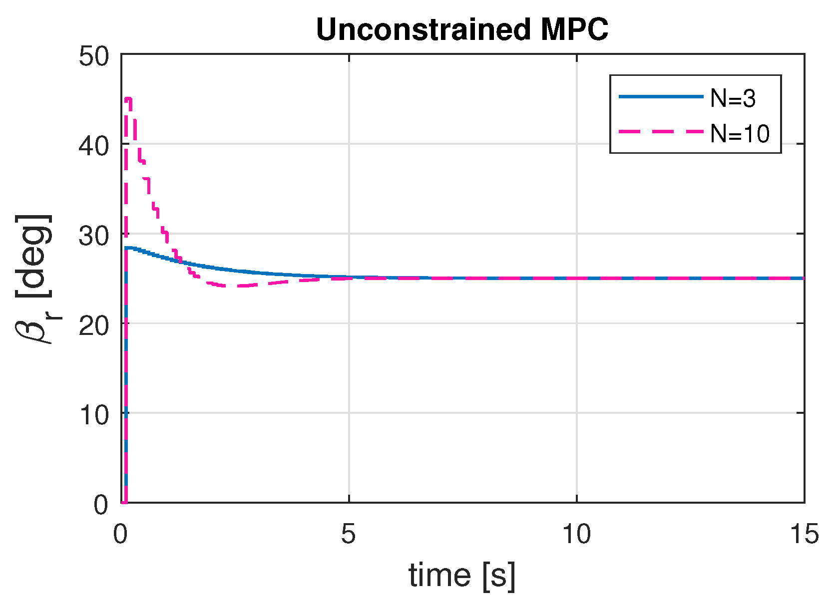
Initially, the unconstrained MPC was simulated using two distinct prediction horizons, denoted as $N=3$ and $N=10$, to analyze the impact of the prediction horizon. The eigenvalues of the resultant closed-loop system are presented in

Table 3. Eigenvalues for a closed-loop wind turbine system.

Eigenvalues	N = 3	N = 10
${\lambda }_1$	0.9251 + 0.0125i	0.8883 + 0.0769i
${\lambda }_2$	0.9251 − 0.0125i	0.8883 − 0.0769i
${\lambda }_3$	0.2452 + 0.0435i	0.2452 + 0.0435i
${\lambda }_4$	0.2452 − 0.0435i	0.2452 − 0.0435i

. The eigenvalues represent the stability characteristics of the closed-loop wind turbine model under the unconstrained MPC with prediction horizons, $N=3$ and $N=10$. Each eigenvalue corresponds to the poles of the wind turbine model’s closed-loop transfer function, which are directly linked to the stability of the wind turbine system. Since the placement of the eigenvalues in the complex plane determines whether the system is stable or unstable, we can see from the values of Table 3 that all the eigenvalues lie inside the unit circle in the complex plane (for the discrete-time model). Therefore, the wind turbine CART model considered in our work operates under stable conditions. The stability condition is further verified by all the simulation results discussed in the following section. The eigenvalues have been computed using MATLAB’s eig() function by simulating the closed-loop wind turbine dynamics using prediction horizons N = 3 and N = 10.

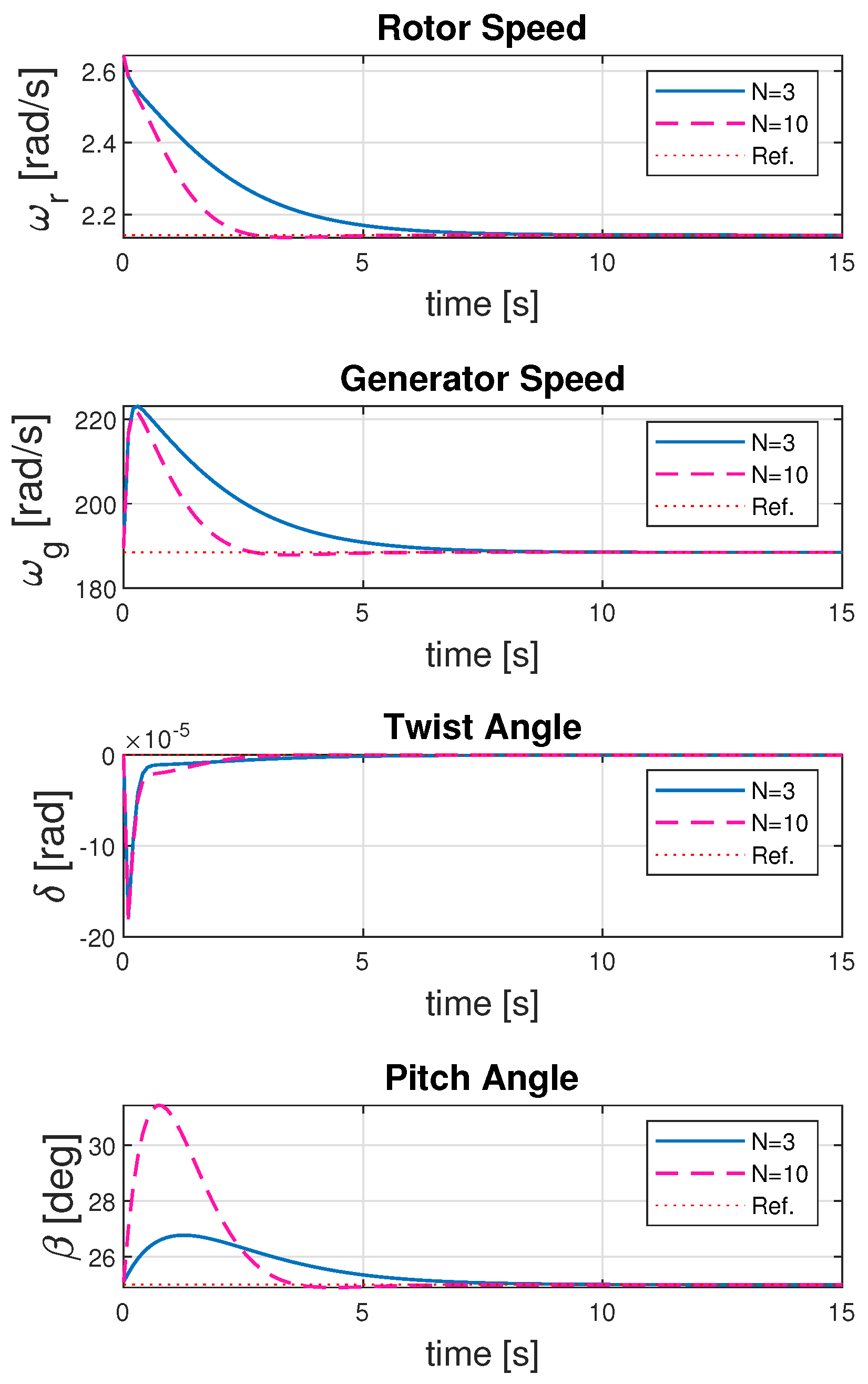
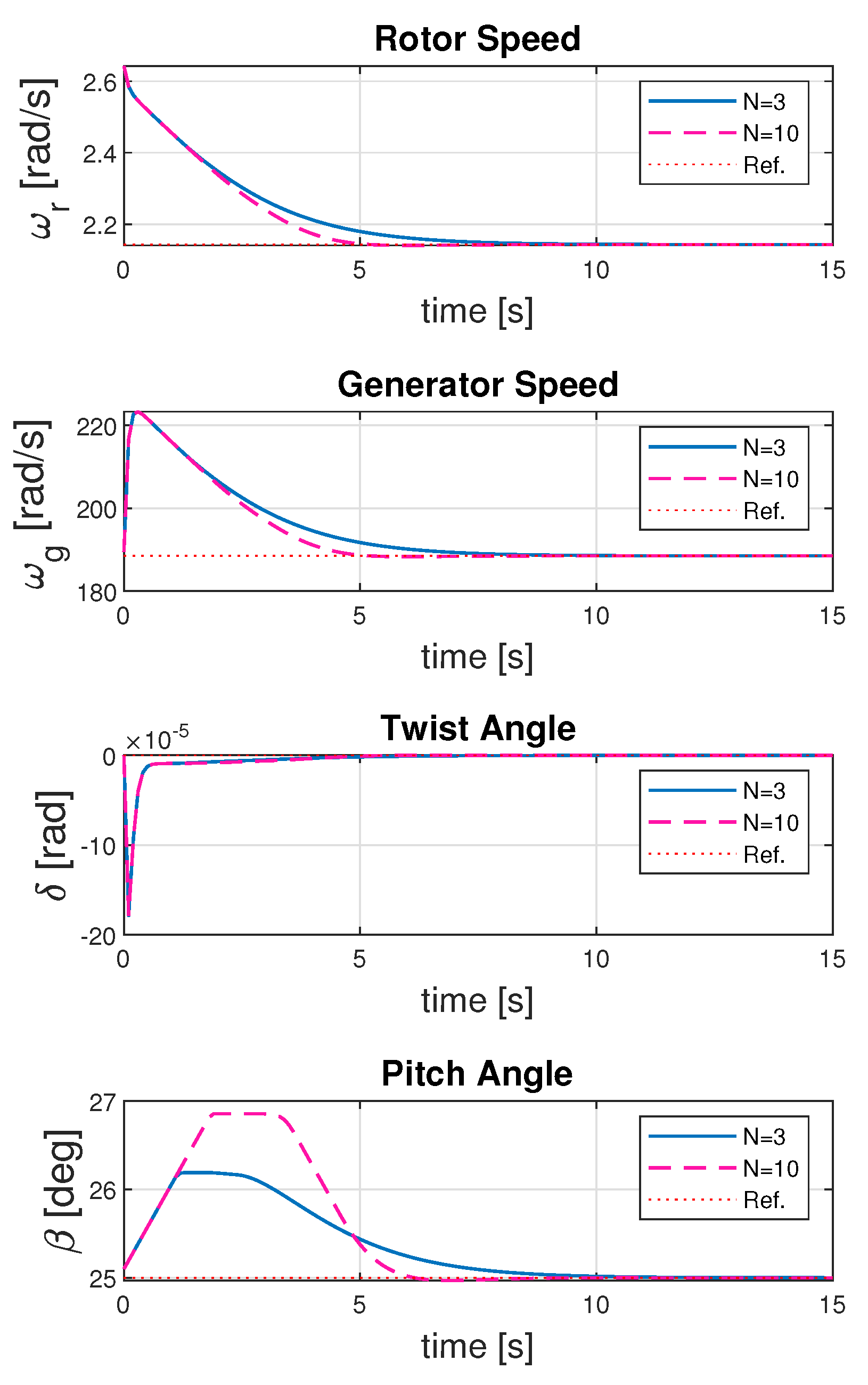
Figure 4 shows the convergence of the states of the wind turbine dynamics to the operating point. It is evident that, when choosing a higher prediction horizon $(N=10)$, the value converges quickly as the control algorithm decides by looking further into the future than before. The longer-term view allows time to make the adjustments as necessary. However, the increase in the convergence rate by choosing a larger prediction horizon results in higher control input for the system, as evident from Figure 5. It is supported numerically from the value of receding horizon control gain in

Table 4. Receding horizon control gain.

N = 3	−6.8072	−0.0166	16.0869	0.2603
N = 10	−40.1319	−0.0689	15.2870	0.9769

. This is justified as the controller tries to compensate for the potential disturbances to the turbine operation over a longer time span and takes more aggressive control action.

In real-world operation, the pitch angle actuator places strict limitations on the wind turbine system in terms of both the magnitude of its movement and how quickly it can change position. The MPC problem takes the constraints of the system as outlined in

Table 5. Constraints.

Parameter	Description	Value
${\beta }_{lim}$	Pitch angle limit	$-1^{\circ }$ to ${90}^{\circ }$
${\dot{\beta }}_{lim}$	Pitch rate limit	$\pm {10}^{\circ }/s$

. The propagation of the states of the system is illustrated in Figure 6. As the prediction horizon extends, the convergence rate also improves, although at a slower pace compared to the unconstrained scenario because of the constraints imposed on the pitch angle rate of change, i.e., how quickly the pitch angle rate of the wind turbine can change. This is considered for the physical limitation and safe operation of the turbine. Similarly, the control input is larger on increasing the prediction horizon, as shown in Figure 7. However, it is less aggressive than the unconstrained case discussed before.

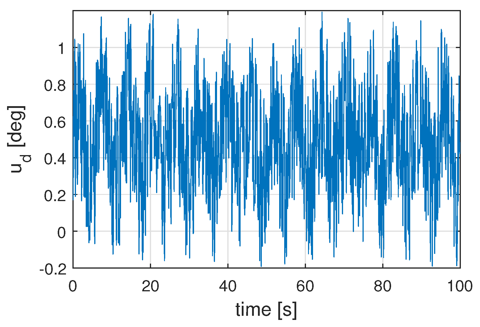
As highlighted in the introduction section, in practice, environmental disturbances impact wind turbines’ operation. The variation could be in wind speed, wind direction, turbulence, etc. We have considered the disturbance signal shown in Figure 8 into the system Equation (13) to study and mitigate the effect of the disturbances on the performance of the wind turbine. The simulation is done with a prediction horizon $N=3$. 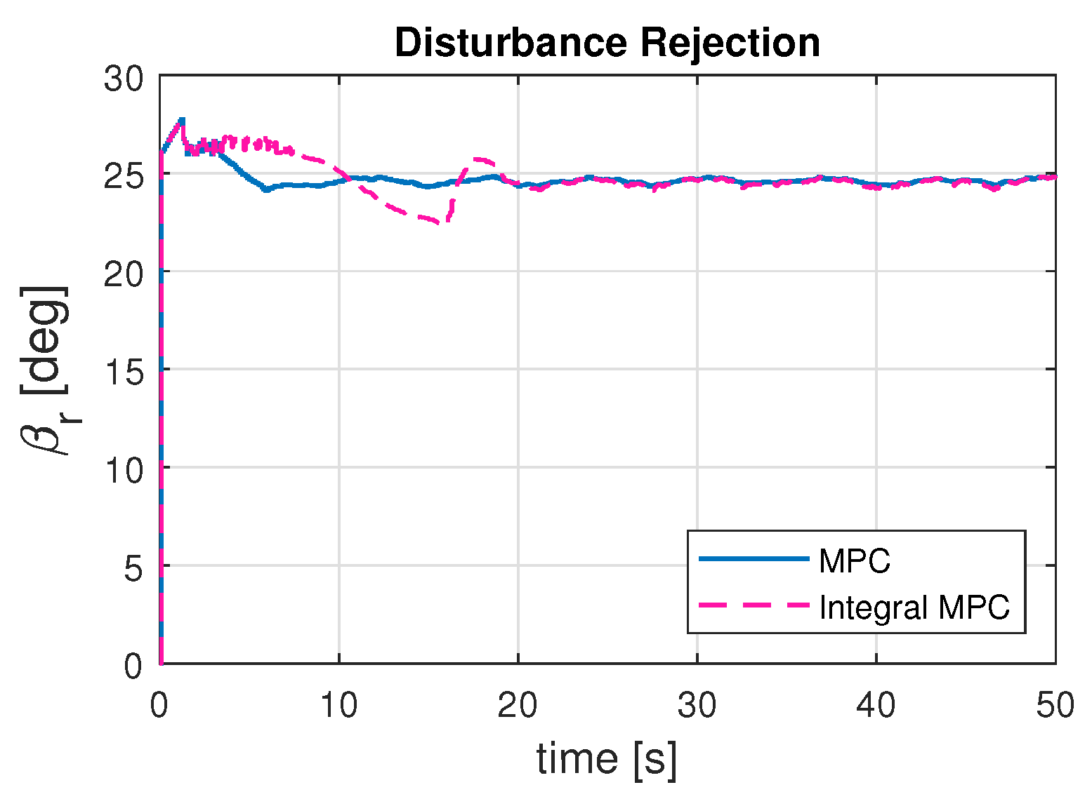In Figure 9, the results are shown in solid lines for the convergence of the system states for the constrained MPC with disturbance rejection. It measures the controller’s adaptability to changing wind conditions and analyzes how quickly the controller acts to the disturbance. The control input is shown in solid blue lines in Figure 10. The controller is working effectively in response to the disturbance to the wind turbine.

Moreover, to further enhance the control performance of the wind turbine for disturbance rejection, we have implemented integral control to reduce the steady-state error of the system. Firstly, it is helpful in rotor speed regulation to maximize the energy capture while maintaining safe operation. Further, it is useful for optimizing the blade pitch angle to control power production and mitigate loads on turbine control. It also regulates the generator torque to maintain the grid stability and maximize the output power. In Figure 9, it can be seen that the steady-state error has decreased by using the integral MPC. This comes at the expense of a reduced convergence rate of the system because the accumulated error influences the control input gradually in the integral MPC, leading to a slower adjustment process. The integral term, as given in Section 3.2, reacts to past errors, which slows down the immediate response to changes. To further quantify the performance comparison of the controllers for the wind turbine system, the value of Integral Absolute Error (IAE) is computed as $IAE=\int \left|e\right|dt$. It is calculated for a $300\mathrm{s}$ simulation time and presented in

Table 6. Integral Absolute Error of States.

Variable	Constrained MPC	Integral MPC
${\omega }_r$	8.0671	2.2428
${\omega }_g$	708.2074	195.8734
$\delta$	0.0001	0.0001
$\beta$	76.4240	37.3294

. It verifies the objective of reducing the steady-state error in the wind turbine operation by using the integral control MPC.

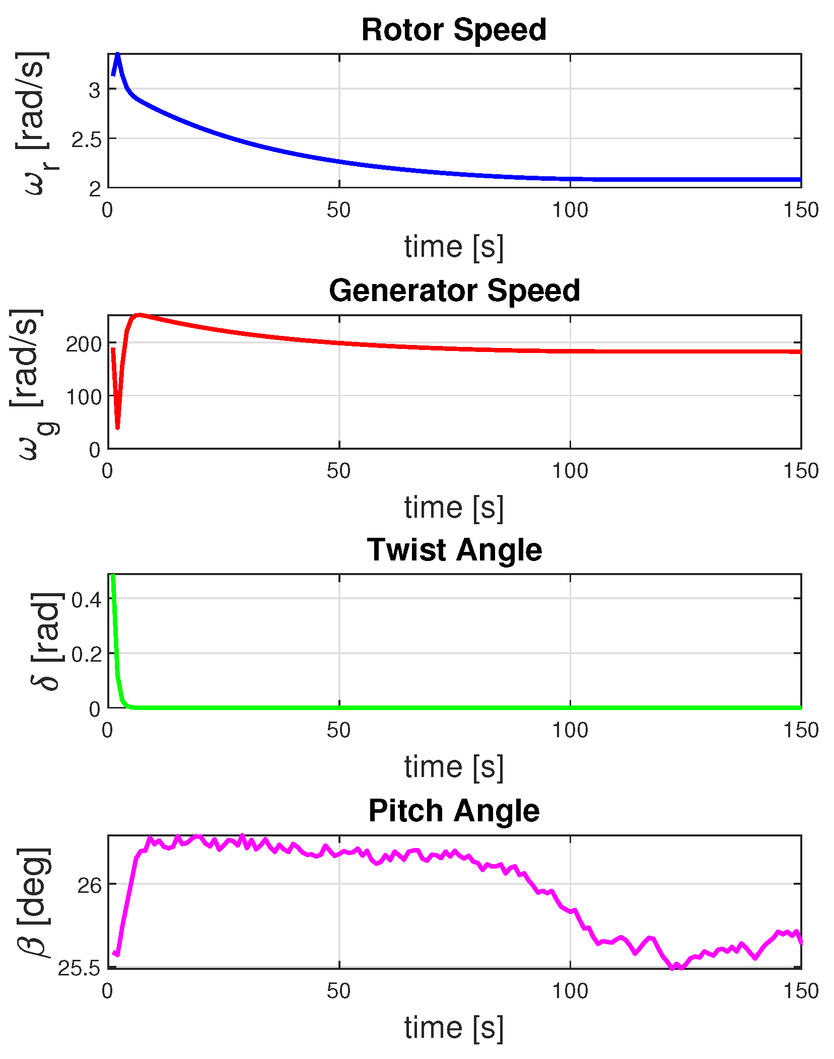
To further verify the effectiveness of the controller action for disturbance rejection, we have obtained the statistical analysis for varying initial conditions of the wind turbine operation. Figure 11 shows the first moment, i.e., mean propagation, and it is evident that the mean propagation of all the states of the wind turbine converges to the designated operating point of the wind turbine, i.e., $\tilde{\mathbf{z}}={\left[\begin{array}{cccc}2.14& 188.4& 0& 25\end{array}\right]}^T$. It shows that the controller can guide the turbine to its desired operational state regardless of initial conditions, even in the presence of disturbance, ensuring reliable performance. It also provides an important aspect of integrating wind power into the larger power grid. The controller action effectively maintains the operating speed of the rotor for energy conversion and stable power generation. The convergence of generator speed ensures grid synchronization and is essential for consistent electrical power output. Effective pitch angle control indicates the adaptability of the wind turbine to disturbance and uncertain environmental conditions, i.e., capturing maximum energy while ensuring longevity. Lastly, the convergence of the twist angle ensures effective aerodynamic performance of the wind turbine system. 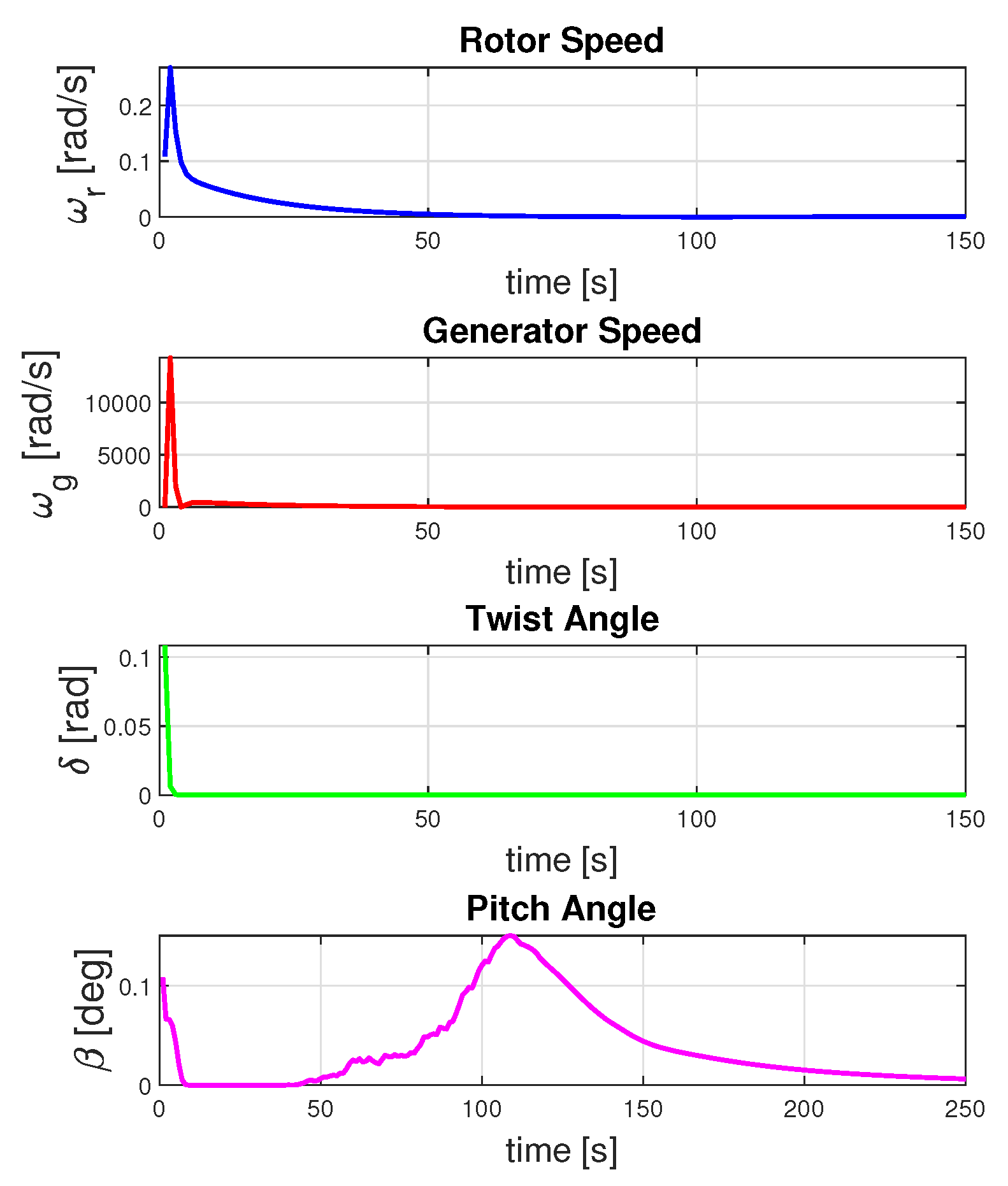Further, in Figure 12, we have shown the variance propagation of all the states of the wind turbine system dynamics. Following the mean propagation analysis, once the states converge to the operating point of a wind turbine, the variance value converges to zero. The convergence of variance to zero for all the states signifies a stable, efficient, and reliable wind turbine operation, enhancing both the performance and longevity of the system.

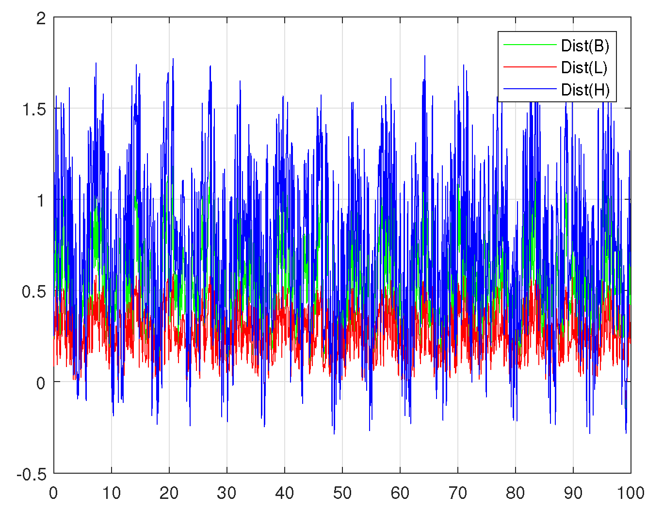
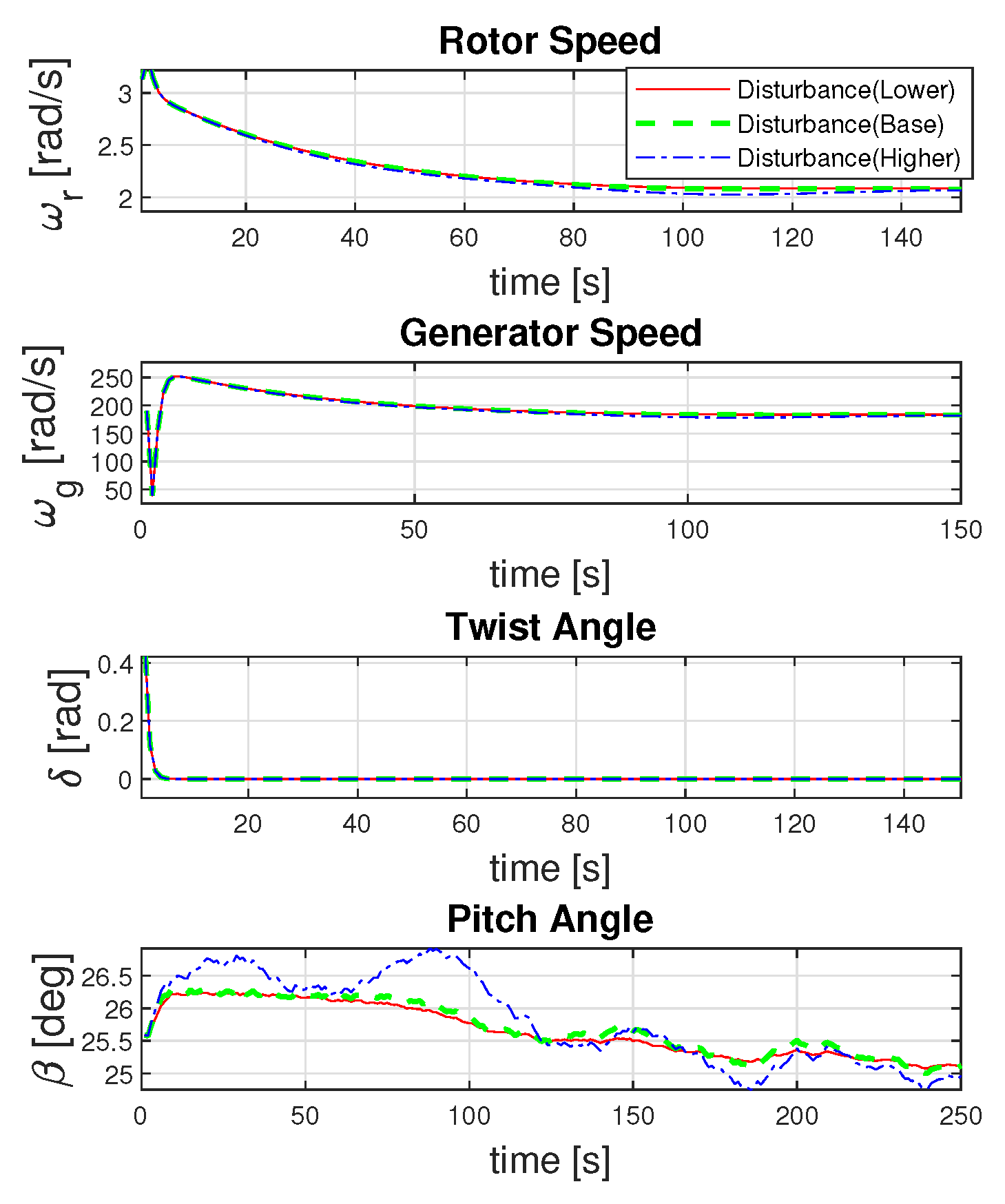
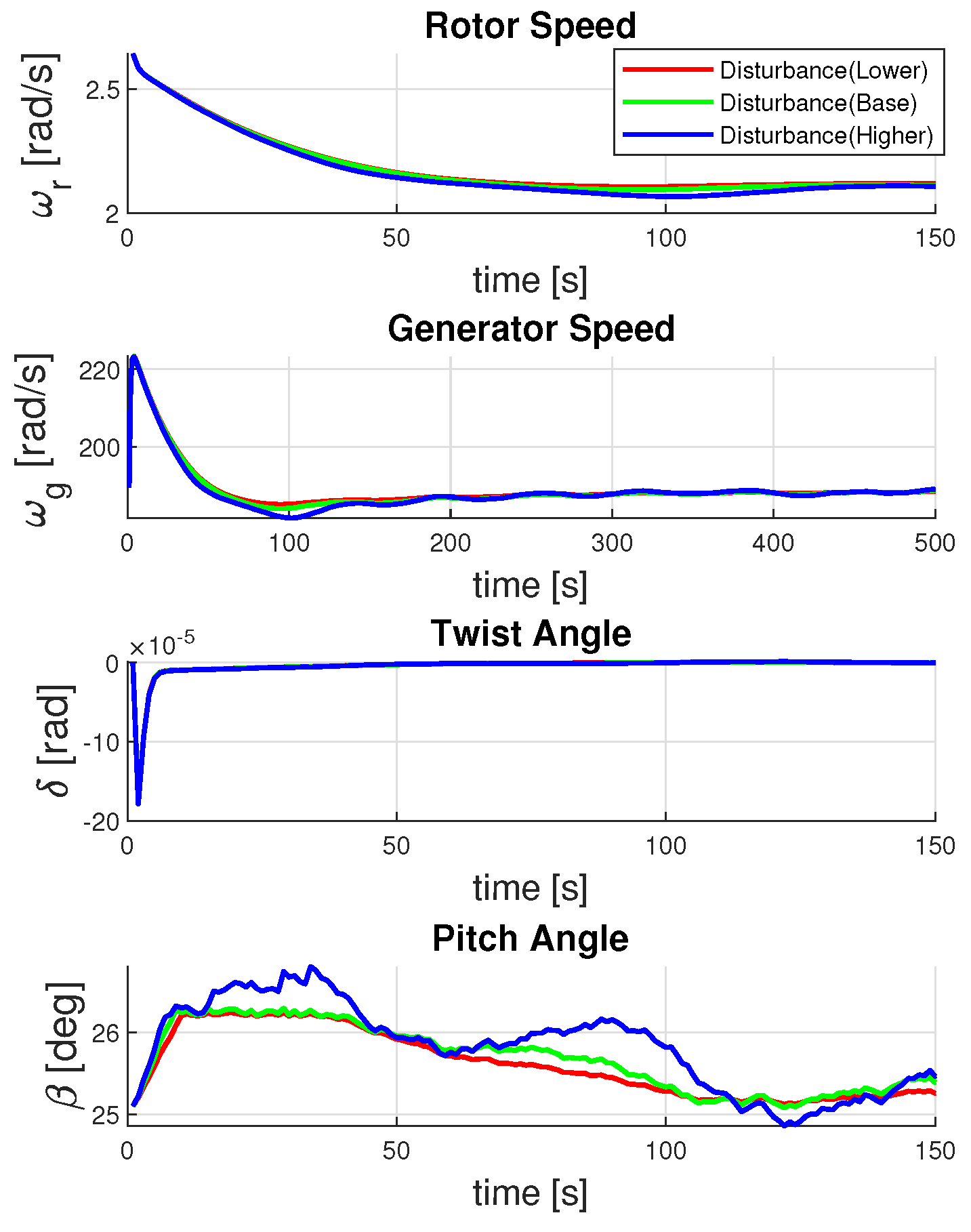
In our work so far, we have shown the effectiveness of the integral MPC for disturbance rejection and uncertain initial conditions. To further consolidate the effectiveness of the controller action, we have considered the variation in the intensity of the disturbance. As shown in Figure 13, the disturbance intensity is varied by $\pm 50\%$ to the intensity shown in Figure 8. The wind turbine system is subjected to both extremes of the disturbance to study the effect of the controller action. In Figure 14, the results for the states of the wind turbine system show that the controller action can guide the system to the designed operating point for both extremes of the disturbance. The results are almost similar in terms of the system’s rotor speed, generator speed, and twist angle. However, the difference in controller action is visible for the pitch angle of the wind turbine. When the disturbance increases, the controller adjusts the pitch angle to reduce the aerodynamic load on the blades, preventing potential damage and maintaining the power output of the system. Conversely, when the disturbance decreases, the pitch angle is adjusted to maximize the energy captured by the wind turbine.

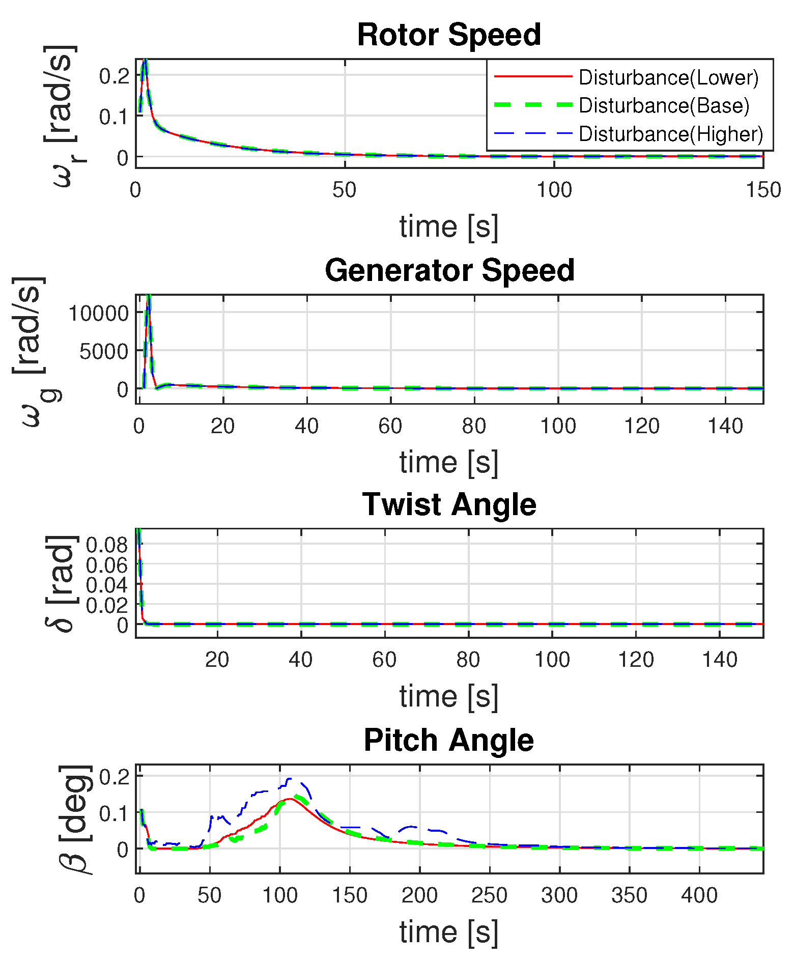
As before, we have considered the case of uncertainty in the initial conditions of the wind turbine operation and obtained the mean and variance propagation for the states of the system. The mean propagation in Figure 15 shows that all the states converge to the designated operating point of the wind turbine, i.e., $\tilde{\mathbf{z}}={\left[\begin{array}{cccc}2.14& 188.4& 0& 25\end{array}\right]}^T$. Figure 16 shows the convergence of variance propagation of all the states to zero once the operating point for the wind turbine has been reached. Overall, we can conclude that the convergence of the mean propagation and the reduction of variance propagation to zero in the state variables under initial condition uncertainties with variable disturbance intensity highlight the effectiveness and robustness of the wind turbine’s integral MPC. It ensures the turbine can achieve and maintain its designated operating point reliably, enhancing performance and operational stability.

6. Conclusions

MPC framework is invaluable in achieving optimal control objectives for wind turbine systems due to its ability to incorporate numerous practical constraints on system states and inputs, its predictive algorithmic nature, and the ability to reject disturbances. In this paper, we developed a linearized model of a wind turbine, which was then employed in formulating an MPC problem to mitigate the effects of disturbances. Our simulation outcomes demonstrate the effectiveness of MPC in meeting specified constraints even when disturbances are present. Additionally, integral control was implemented to minimize the wind turbine system’s steady-state error. We also show the control action for the uncertain initial conditions of the states of the wind turbine. The mean and variance propagation shows the effectiveness of the designed controller for the operation of the wind turbine system. Further, the results obtained for the variable disturbance intensity and uncertain initial conditions showed the effect of MPC on enhancing performance and operation stability. The results are discussed using the deterministic uncertainty for the computationally efficient and systematic exploration of the wind turbine’s dynamic response. Our goal in this work was to establish foundational insights into the effect of specific disturbances, emphasizing rejection using the MPC algorithm framework, serving as a basis for potential future probabilistic studies.

In future work, we plan to explore the random sampling approach to complement the deterministic analysis and provide a more robust uncertainty quantification for the wind turbine model. Moreover, the obtained results are promising for further implementation of the proposed approach in real wind farms, which can be achieved by integrating it into existing turbine control architectures with real-time optimization capabilities. However, some practical challenges may require detailed analysis for successful implementation, such as wind turbine model accuracy, computational demands for the extensive system, and reliable wind disturbance estimation. We will be looking to address these challenges in future work. One possible solution to explore is to develop an operator-theoretic data-driven model of wind turbines, including developing MPC algorithms robust to stochastic wind speed disturbance.