Short-Term Power Load Forecasting Using Adaptive Mode Decomposition and Improved Least Squares Support Vector Machine

Abstract

Accurate power load forecasting is crucial for ensuring grid stability, optimizing economic dispatch, and facilitating renewable energy integration in modern smart grids. However, real load forecasting is often disturbed by the inherent non-stationarity and multi-factor coupling effects. To address this problem, a novel hybrid forecasting framework based on adaptive mode decomposition (AMD) and improved least squares support vector machine (ILSSVM) is proposed for effective short-term power load forecasting. First, AMD is utilized to obtain multiple components of the power load signal. In AMD, the minimum energy loss is used to adjust the decomposition parameter adaptively, which can effectively decrease the risk of generating spurious modes and losing critical load components. Then, the ILSSVM is presented to predict different power load components, separately. Different frequency features are effectively extracted by using the proposed combination kernel structure, which can achieve the balance of learning capacity and generalization capacity for each unique load component. Further, an optimized genetic algorithm is deployed to optimize model parameters in ILSSVM by integrating the adaptive genetic algorithm and simulated annealing to improve load forecasting accuracy. The real short-term power load dataset is collected from Guangxi region in China to test the proposed forecasting framework. Extensive experiments are carried out and the results demonstrate that our framework achieves an MAPE of 1.78%, which outperforms some other advanced forecasting models.

1. Introduction

Power load forecasting has long been a critical research topic in electrical engineering, serving as the cornerstone for strategic power system planning and real-time operational optimization [1,2]. Among its subfields, short-term load forecasting (STLF) assumes particular significance, providing indispensable guidance for generation scheduling, demand-side management, and market-based electricity trading mechanisms [3,4]. In recent years, the increasing integration of renewable energy has led to more complex and diversified load characteristics in power grids, significantly heightening the challenges of accurate load forecasting [5,6]. To maintain power grid operational reliability and economic efficiency, effective and reliable STLF strategies need to be explored.

1.1. STLF Method

According to the related literature review, in recent decades, research on STLF has yielded a multitude of robust methodologies [7]. Based on the technical principles and empirical validation, these methodologies can be classified into three primary categories: mathematical statistics-based, artificial intelligence-based, and hybrid methodologies [8]. Common mathematical statistics-based methodologies contain the exponential smoothing model [9], autoregressive integrated moving averages (ARIMA) [10], and linear regression analysis [11]. These mathematical statistics-based methodologies have the advantages of simple structure, fast calculation speed, and easy explanation. However, the forecasting accuracy is limited for nonlinear series, which cannot meet the requirement for non-stationary STLF [8]. Therefore, more effective methods are in demand.

With the rapid advancement of computational capabilities, the artificial intelligence-based methodologies have been widely used in STLF [12]. The artificial intelligence-based methodologies include machine learning [13] and deep learning methods [14]. Unlike conventional mathematical statistics-based methodologies, these artificial intelligence-based methodologies demonstrate superior capability in dealing with nonlinear and non-stationarity problems [15,16]. Some popular methods are support vector machine (SVM), artificial neural networks (ANNs), convolutional neural networks (CNNs) and their improved structures, and so on [17]. In [18], the ANN model was utilized to predict the power load, where similar day methods were presented to improve the accuracy of STLF. In [19], one-dimensional (1-D) CNN and deep residual network (ResNet) were combined to build a parallel STLF model, in which the 1-D CNN was used for feature extraction and the ResNet was utilized to improve generalization performance. Recently, a CNN-LSTM model with multi-modal attention mechanism was proposed and applied for power grid load forecasting [20].

These artificial intelligence-based methodologies have provided convenience for STLF. However, their accuracies strongly depend on effective feature information. To address this, some hybrid models were developed by introducing some signal decomposition techniques such as variational mode decomposition (VMD) [21], empirical mode decomposition (EMD) [22], and ensemble empirical mode decomposition (EEMD) [23]. For example, the VMD and bidirectional long short-term memory (BiLSTM) were combined to predict short-term power load, where the VMD was used to extract load features so as to improve the forecasting performance of BiLSTM in [24]. Additionally, the EMD and LSTM were selected to conduct a hybrid model for sub-hourly load forecasting in [25].

1.2. Research Gap and Contributions

Some problems also need to be considered for hybrid STLF methods. For example, signal decomposition techniques are often affected by decomposition numbers. Unsuitable decomposition numbers may lose some critical load components or introduce other extra information, reducing load feature effectiveness. The deep learning methods such as neural networks also have some drawbacks for STLF. For instance, they often require large datasets for stable training and are prone to overfitting in small-sample regimes. Moreover, the black-box structure makes it difficult to provide clear interpretation.

Unlike neural networks, the SVM can effectively obtain feature information with a lower data consumption [26]. As an improvement of SVM, least squares support vector machine (LSSVM) is often considered for power load forecasting [27]. LSSVM adopts the structural risk minimization principle, which balances model complexity and empirical error, effectively mitigating overfitting. Additionally, it provides mathematically tractable solutions through kernel-based regression, enabling effective interpretation of load dynamics. For instance, an LSSVM with dynamic particle swarm optimization algorithm was used for STLF in [28]. Nevertheless, the LSSVM has a high dependency on kernel functions and parameters. Because the load sequence contains multiple frequency components, a fixed kernel function has difficulty meeting the forecasting requirement. Furthermore, the forecasting accuracy of LSSVM is sensitive for model parameters. Therefore, some improvement methods need to be further developed.

As a solution to the abovementioned problem, this work proposes an effective hybrid framework for STLF and our contributions are listed as follows:

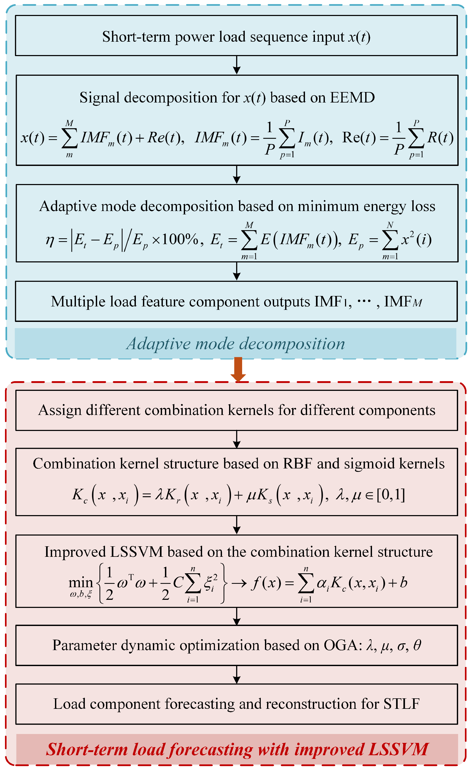
• To extract effective load information, an adaptive mode decomposition (AMD) based on EEMD is proposed to obtain different feature components. In AMD, the decomposition parameter can be adjusted dynamically based on minimum energy loss, contributing to an optimal decomposition.
• To fully consider the diversities of different load components, an improved least squares support vector machine (ILSSVM) is proposed to learn critical information for STLF. Particularly, a combination kernel structure and optimized genetic algorithm (OGA) were presented to further enhance model performance.
• A hybrid framework for STLF is further presented based on AMD and ILSSVM. In this framework, different load components can be assigned different combination kernel functions, which can significantly improve forecasting accuracy so as to support energy planning and operation.

The remainder of this article is organized as follows: the AMD is presented in Section 2. Section 3 proposes the ILSSVM model. Then, the framework for STLF is described in Section 4. In Section 5, experiments are carried out for verification analysis. Finally, Section 6 concludes this article.

2. Adaptive Mode Decomposition

2.1. Principle of AMD

The intricate dynamics of power load sequences, marked by inherent nonlinear and non-stationary attributes, pose significant challenges for precise STLF, demanding advanced multiscale feature extraction methods. EMD has emerged as a prominent analytical technique in this domain, decomposing raw power load sequences into multiple intrinsic mode functions (IMFs). These IMFs contain multiple different frequency data points, which are critical for non-stationary load sequence analysis. However, conventional EMD implementations remain prone to mode mixing, which is a critical drawback that may introduce some extra frequency components during decomposition, particularly when processing multicomponent load sequences. To address this limitation, the EEMD methodology is introduced, leveraging a noise-assisted ensemble strategy where multiple EMD trials are executed with adaptively injected white noise variants. By averaging resultant IMF sets across iterations, EEMD effectively suppresses spurious mode generation while enhancing decomposition consistency.

For the load sequence $x\left(t\right)$, in each trial, the EMD is executed and an independent white noise ${\mu }_p\left(t\right)$ is injected. Denote the number of trials as P, and the load sequence can be modified as

$$x_p\left(t\right)=x\left(t\right)+{\mu }_p\left(t\right),p=1,2,...,P$$

(1)

By executing the EMD process, the load sequence is decomposed, where multiple IMFs $I_m\left(t\right)$ and a residual $R_p\left(t\right)$ are obtained [25]. Then, the load sequence in (1) is decomposed and can be expressed as

$$x_p\left(t\right)=\sum _{m=1}^M{I}_m\left(t\right)+R_p\left(t\right)$$

(2)

where M represents the decomposition number of IMFs.

The idea of EEMD is to compute the mean of different IMFs and residuals after multiple EMD trials, which can effectively overcome the disturbance of the white noise ${\mu }_p\left(t\right)$. Based on the EMD process, the IMFs and residuals after EEMD operation for load sequence can be further described as

$$IM{F}_m\left(t\right)={\displaystyle \frac{1}{P}}\sum _{p=1}^P{I}_m\left(t\right)$$

(3)

$$Re\left(t\right)={\displaystyle \frac{1}{P}}\sum _{p=1}^P{R}_p\left(t\right)$$

(4)

where $IM{F}_m\left(t\right)$ represents the mth load component.

Based on the above description, the load sequence EEMD result can be given as

$$x\left(t\right)=\sum _{m=1}^{M}IM{F}_m\left(t\right)+Re\left(t\right)$$

(5)

Compared with EMD, EEMD significantly reduces noise interference and mitigates mode aliasing through iterative noise-assisted averaging, facilitating accurate isolation of power load components. However, traditional EEMD implementations relying on fixed IMF selection criteria risk generating spurious modes or losing critical load components. To resolve this, an adaptive mode decomposition is proposed, which autonomously adjusts IMF quantities and optimizes decomposition fidelity under varying grid conditions.

2.2. Proposed AMD

Non-stationary load signals often exhibit energy redistribution across scales due to factors like renewable generation intermittency. Minimizing energy loss ensures that the residual contains only non-oscillatory trends, aligning with the physical definition of IMFs in EEMD-based methods. The energy loss criterion inherently captures the nonlinear coupling effects in load curves: High-frequency IMFs correspond to stochastic components with low energy persistence. Low-frequency IMFs exhibit energy concentration in specific bands, which is consistent with Fourier–Bessel spectral analysis in adaptive wavelet methods. This matches the “adaptive filter bank” behavior observed in VMD when processing non-stationary signals.

When the M is too small, it is easy to result in mode mixing and incomplete trend extraction. Insufficient M fails to separate overlapping frequency components. This results in IMFs containing mixed oscillations from different physical processes, violating the IMF definition of representing distinct oscillatory modes. Additionally, critical power load signal components with small energy contributions may be discarded prematurely, leading to information loss. When the M is too large, it tends to decompose stochastic noise into high-frequency IMFs, generating spurious modes that lack physical correspondence to underlying signal drivers. Consequently, improper specification of decomposition parameters may induce non-physical energy dissipation, manifesting as diminished aggregate energy preservation across the derived IMFs when compared to the original signal’s total energy content. In this way, the energy loss will increase when the decomposition number M is too large or too small.

The fundamental objective of AMD lies in minimizing post-decomposition energy loss while maintaining fidelity to the energy conservation principle, which dictates that the cumulative energy of IMFs should equate to the original energy of load sequence [29]. The optimal decomposition number M is achieved when the energy loss achieves minimum, which is defined as when the normalized difference between load input and reconstructed signal energies is minimized through iterative parameter optimization. Thus, AMD can effectively avoid critical load component loss and further mitigate the potential for creating such spurious components by obtaining minimum energy loss.

For the power load sequence $x\left(t\right)$, its energy is defined as

$$E_p=\sum _{i=1}^N{x}^2\left(i\right)$$

(6)

where $x\left(i\right)$ and N represent the amplitude in the i-th point and the number of all points, respectively.

The total energy of all IMFs after the EEMD process can be computed as

$$E_t=\sum _{m=1}^{M}E\left(IM{F}_m\left(t\right)\right)$$

(7)

there is

$$E\left(IM{F}_m\left(t\right)\right)=\sum _{i=1}^{N}IM{F}_m^2\left(i\right)$$

(8)

where $E_t$ and $E\left(IM{F}_m\left(t\right)\right)$ represent the total energy and the energy of the m-th IMF, respectively.

Based on the load sequence energy change before and after decomposition, the energy loss is defined as

$$\eta ={\displaystyle \frac{|E_t-E_p|}{E_p}}\times 100\%$$

(9)

In AMD, the original total energy of load sequence is fixed, and when the energy loss obtains the minimum, the corresponding decomposition number is optimal. In this way, the decomposition process is more flexible and can provide more effective power load information.

After the AMD process, a proper prediction model is needed for STLF. Next, an improved least squares support vector machine (ILSSVM) is presented to fully consider the diversities of different load components.

3. Improved Least Squares Support Vector Machine

3.1. Principle of LSSVM

LSSVM, a computationally efficient variant of the conventional SVM, is developed to streamline computational procedures and enhance algorithmic efficiency. Its fundamental innovation lies in replacing inequality constraints with equality constraints while incorporating a quadratic error term into the optimization objective. The regression function can be described as

$$f\left(x\right)={\omega }^{\mathrm{T}}\phi \left(x\right)+b$$

(10)

where $\omega$ denotes the weight, b denotes the bias, x is the input, and $\phi \left(\right)$ denotes the map function.

The LSSVM fundamentally restructures the convex optimization framework of conventional SVM by substituting inequality constraints with equality counterparts. The optimization objective of LSSVM can be described as

$$\underset{\omega ,b,\xi }{min}J(\omega ,\xi )={\displaystyle \frac{1}{2}}{\omega }^{\mathrm{T}}\omega +{\displaystyle \frac{1}{2}}C\sum _{i=1}^n{\xi }_i^2$$

(11)

subjected to

$$y_i={\omega }^{\mathrm{T}}\phi \left(x_i\right)+b+{\xi }_{i}i=1,2,\dots ,n$$

(12)

where $\xi$ is the slack variable, C is the penalty coefficient, and n is the sample size.

The Lagrange function is introduced, described as

$$L\left(\omega ,b,{\xi }_{,}\alpha \right)={\displaystyle \frac{1}{2}}{\omega }^{\mathrm{T}}\omega +{\displaystyle \frac{1}{2}}C\sum _{i=1}^n{\xi }_i^2-\sum _{i=1}^n{\alpha }_i\left[{\omega }^{\mathrm{T}}\phi \left(x_i\right)+b+{\xi }_i-y_i\right]$$

(13)

where ${\alpha }_i$ denotes Lagrange multiplier.

After solving the partial differential, the regression prediction function of LSSVM can be described as

$$f\left(x\right)=\sum _{i=1}^n{\alpha }_{i}K\left(x,x_i\right)+b$$

(14)

where K(,) is the kernel function.

3.2. Proposed ILSSVM

Generally, the kernel function directly affects the forecasting performance of LSSVM. Nevertheless, traditional the LSSVM model adopts a single-kernel structure for feature mapping. The power load sequence contains different frequency components, which indicates that it is difficult to consider feature diversity by using the same kernel structure. Moreover, the utilization of a single-kernel function inherently imposes a fundamental trade-off between model learning capacity and generalization capability, often failing to concurrently optimize both aspects in complex pattern recognition tasks. To address this, the first improvement of ILSSVM is using a combination kernel structure for STLF.

In this research, two types of kernel functions are selected to produce the combination kernel structure. One is the Radial Basis Function (RBF) kernel with a high learning capacity, which can achieve near-universal approximation capability, which can be defined as

$$K_r\left(x,x_i\right)=exp\left(-{\displaystyle \frac{{∥x-x_i∥}^2}{2{\sigma }^2}}\right)$$

(15)

where $\sigma$ is the RBF kernel width.

The other is the sigmoid kernel with a satisfactory generalization capability, which can be defined as

$$K_s\left(x,x_i\right)=tanh\left[x^{\mathrm{T}}{x}_i+\theta \right]$$

(16)

where $\theta$ is the sigmoid kernel parameter.

Based on (15) and (16), the combination kernel structure is designed for STLF, which can be described as

$$K_c\left(x,x_i\right)=\lambda K_r\left(x,x_i\right)+\mu K_s\left(x,x_i\right)$$

(17)

where $\lambda ,\mu$ are kernel weights and range from 0 to 1.

From (17), the combination kernel structure can effectively extract different load component information by adjusting kernel weights. A higher $\lambda$ indicates an emphasis on learning capability, while a higher $\mu$ focuses on the generalization capability. In this way, the combination kernel structure can provide a more flexible feature extraction performance for STLF.

Utilizing the combination kernel, the final regression prediction function of ILSSVM can be given as

$$f\left(x\right)=\sum _{i=1}^n{\alpha }_i{K}_c\left(x,x_i\right)+b$$

(18)

In ILSSVM, the combination kernel structure can improve its flexibility for load forecasting, but more model parameters are introduced including kernel weights $\lambda$, $\mu$, and kernel parameters $\sigma$, and $\theta$. To avoid the impact of these parameters, the other improvement of ILSSVM is adjusting these model parameters adaptively based on the proposed optimized genetic algorithm (OGA). Motivated by [30], an adaptive genetic algorithm is first used as the basis of the OGA, where the crossover probability $P_c$ and mutation probability $P_m$ can be dynamically adjusted with evolution. In this way, it can significantly mitigate the risk of becoming trapped in local optima. For the parameter setting of ILSSVM, the crossover probability $P_c$ and mutation probability $P_m$ can be described as

While $f_{\mathrm{avg}}\le f^{\prime },f<f_{max}$,

$$P_c={\rho }_3-\left({\rho }_3-{\rho }_2\right)exp\left(1-{\displaystyle \frac{f_{max}-f_{\mathrm{avg}}}{f_{max}-f^{\prime }}}\right)$$

(19)

$$P_m={\gamma }_3-\left({\gamma }_3-{\gamma }_2\right)exp\left(1-{\displaystyle \frac{f_{max}-f_{\mathrm{avg}}}{f_{max}-f}}\right)$$

(20)

While $f_{min}\le f^{\prime },f<f_{\mathrm{avg}}$,

$$P_c={\rho }_1+{\displaystyle \frac{{\rho }_2-{\rho }_1}{1+exp\left(A\frac{2\left(f_{\mathrm{avg}}-f^{\prime }\right)}{f_{\mathrm{avg}}-f_{min}-1}\right)}}$$

(21)

$$P_m={\gamma }_1+{\displaystyle \frac{{\gamma }_2-{\gamma }_1}{1+exp\left(A\frac{2\left(f_{\mathrm{avg}}-f\right)}{f_{\mathrm{avg}}-f_{min}-1}\right)}}$$

(22)

where ${\rho }_1,{\rho }_2,{\rho }_3,{\gamma }_1,{\gamma }_2,{\gamma }_3,A$ are preset parameters, ${\rho }_1<{\rho }_2<{\rho }_3$, ${\gamma }_1<{\gamma }_2<{\gamma }_3$, and $f_{min},f_{\mathrm{avg}},f_{max}$ are minimum, average, and maximum population fitness, respectively.

Based on (19) to (22), the AGA introduces a fitness-dependent probability modulation mechanism to optimize stochastic search dynamics, which can provide a satisfactory global search performance. To further enhance its local learning capability, the OGA introduces simulated annealing (SA) to update the subpopulation population of AGA.

In our work, some trials are carried out and the result shows that when the population size is set to 100 and the iteration is set to 200, the change in the overall framework’s accuracy is not obvious with the increases in the population size and iterations. To achieve an optimal balance between search precision and computational efficiency, the population size and iteration number are ultimately configured at 100 and 200, respectively. The optimization process of the OGA in ILSSVM is listed as follows:

• The parameters of ILSSVM are selected as the individual ${\nu }_i$, ${\nu }_i=\{{\lambda }_i,{\mu }_i,{\sigma }_i,{\theta }_i\}$. The size of population Z and number of iterations are set to 100 and 200, respectively, $Z=\{{\nu }_1,{\nu }_2,...,{\nu }_i,...,{\nu }_{100}\}$, ${\rho }_1,{\rho }_2,{\rho }_3,{\gamma }_1,{\gamma }_2,{\gamma }_3$ are set to 0.3, 0.6, 0.9, 0.01, 0.05, and 0.1, respectively. The initial temperature $T_0$ and final temperature $T_f$ are set to 100, and 5, respectively, and the temperature decrease factor $\beta$ is set to 0.8.
• Select the mean absolute percentage error (MAPE) of ILSSVM for STLF as fitness function. Next, solve the $f_{min},f_{\mathrm{avg}},$ and $f_{max}$; the selection strategy in OGA is elite retention and tournament rules. Adjust the crossover probability $P_c$ and mutation probability $P_m$ based on (19) to (22) and then execute crossover and mutation for generating subpopulation $Z_1$.
• Update the subpopulation $Z_1$ based on the Metropolis criterion in SA. Then, repeat step 2 and step 3 until the iteration ending. At this time, the minimum fitness value in the current population is the optimal solution of ILSSVM.

By using the OGA, parameters in ILSSVM can be optimized adaptively. Next, a novel combination framework based on AMD and ILSSVM is further presented for effective short-term load forecasting.

4. Framework for Short-Term Load Forecasting

Using the proposed AMD and ILSSVM, this section proposes a hybrid framework for short-term power load forecasting. The framework is displayed in Figure 1 and the execution pseudocode is given in Algorithm 1, which can be described as follows:

• Load sequence decomposition: Decompose power load sequence by using the AMD method, which can adaptively determine load decomposition number based on minimum energy loss. Then, multiple load components are selected as input information of the forecasting model.
• Short-term load forecasting: Establish an ILSSVM model and assign different combination kernels for different load components. The parameters of ILSSVM can be dynamically adjusted using OGA. Then, forecast different load components and reconstruct these components to achieve short-term load forecasting.

Figure 1. Short-term load forecasting framework based on AMD-ILSSVM.

Figure 1. Short-term load forecasting framework based on AMD-ILSSVM.

It is worth mentioning that the framework decomposes the non-stationary load signal into multiple components and then predicts them independently before reconstruction. On the one hand, the AMD decomposes raw load sequences into IMFs and residuals, effectively isolating high-frequency noise from low-frequency trends. On the other hand, the decomposed IMFs represent distinct temporal scales, enabling tailored modeling for each frequency band. Moreover, multi-factor coupling often induces overlapping frequency components in raw load data. AMD disentangles these coupled modes into independent IMFs, allowing for explicit separation of interacting factors. This decoupling reduces prediction bias caused by intertwined factors.

Algorithm 1: AMD-ILSSVM

1:  Input 2:    The short-term power load sequence, $x\left(t\right)$ 3:  Load signal decomposition 4:    Compute signal energy before decomposition          $E_p={\sum }_{i=1}^N{x}^2\left(i\right)$ 5:    For the maximum decomposition number 6:      M←Calculate energy loss $\eta$(M) to get the optimal decomposition number          $\eta ={\displaystyle \frac{|E_t-E_p|}{E_p}}\times 100\%$ 7:      Load signal decomposition using AMD 8:    End for 9:    Obtain multiple load components 10: Establish the ILSSVM model        $K_c\left(x,x_i\right)=\lambda K_r\left(x,x_i\right)+\mu K_s\left(x,x_i\right)$        $f\left(x\right)={\sum }_{i=1}^n{\alpha }_i{K}_c\left(x,x_i\right)+b$ 11: Set MAPE as forecasting evaluation criterion 12: Model parameter optimization using OGA 13: Output 14:     Load component forecasting and result reconstruction

Thereby, extensive experiments are carried out to verify the proposed short-term load forecasting framework.

5. Experimental Analysis

To validate the proposed short-term load forecasting framework based on AMD and ILSSVM, various experiments are conducted for comparison analysis. The mean absolute percentage error (MAPE) is selected as the load forecasting evaluation criterion, which can provide an intuitive, scale-independent measure that facilitates direct performance comparisons across heterogeneous datasets and power systems with varying load magnitudes.

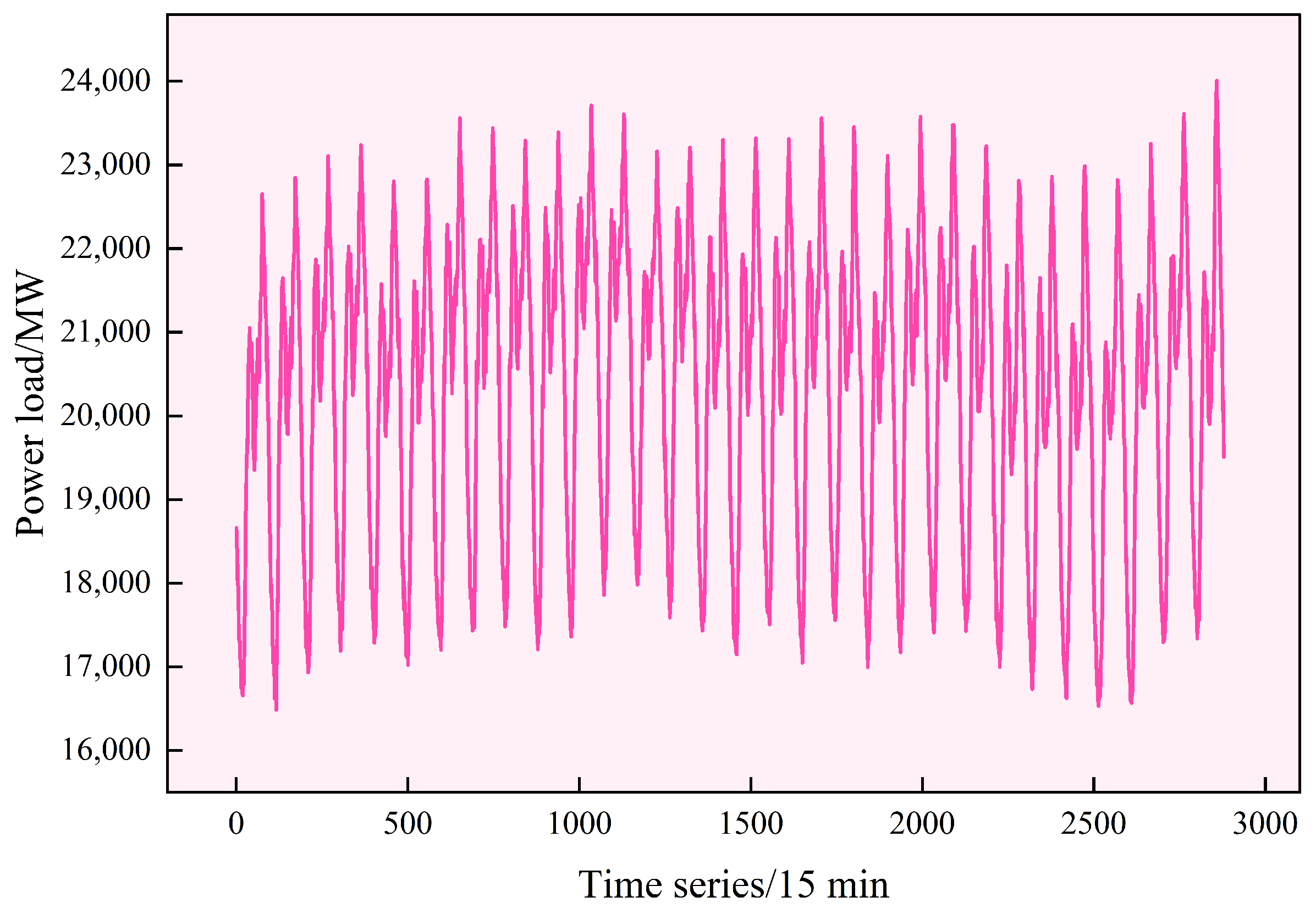
5.1. Experiment Data and Settings

The actual power load used in this research comes from Guangxi region in China and the time ranges from 1st November to 30th November in 2022 with the interval of 15 min, which is displayed in Figure 2. It is worth mentioning that the time sequence ‘1’ in Figure 2 represents the time of 0:00 on 1 November. The ‘2’ represents the time of 0:15 on 1 November, and the last number represents 23:45 on 30 November. From Figure 2, it visually shows the non-stationary and nonlinear characteristics of the power load sequence.

In our experiments, the power load dataset is divided into three parts, where 60% is used for training, 20% is used for validation, and the last 20% is used for testing. Additionally, 5-fold cross-validation is used to avoid overfitting and improve the efficiency of load information utilization. The LS-SVMlab is selected to conduct the ILSSVM model in MATLAB R2022a.

In our work, the assumptions primarily encompass two aspects. The first is that load sequences inherently contain nonlinear and non-stationary components separable via AMD. The other is that the decomposed subseries can be effectively modeled by ILSSVM within a reproducing kernel Hilbert space, where structural risk minimization ensures robustness against overfitting in small-sample regimes. The computational complexity for ILSSVM arises from solving a linear system equation with $O\left(n^3\right)$ operations for n training samples, driven by matrix inversion in the kernel space. Moreover, the potential errors stem from kernel-induced bias in LSSVM, where signal kernel assumptions may mismatch transient load dynamics, and residual mode mixing in EEMD decomposition affecting input quality. We address these through combination kernel structure in ILSSVM and adaptive decomposition number in AMD.

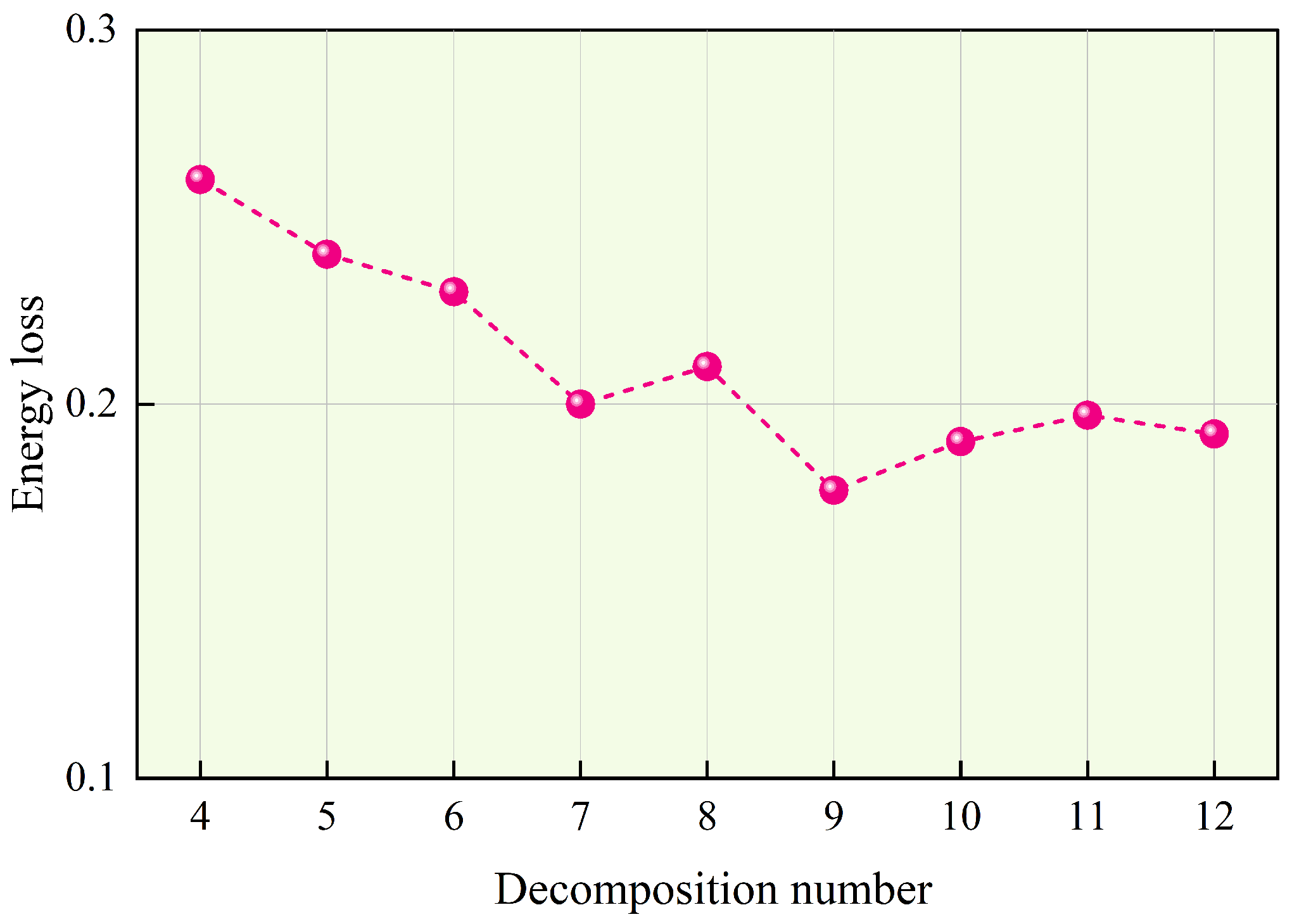
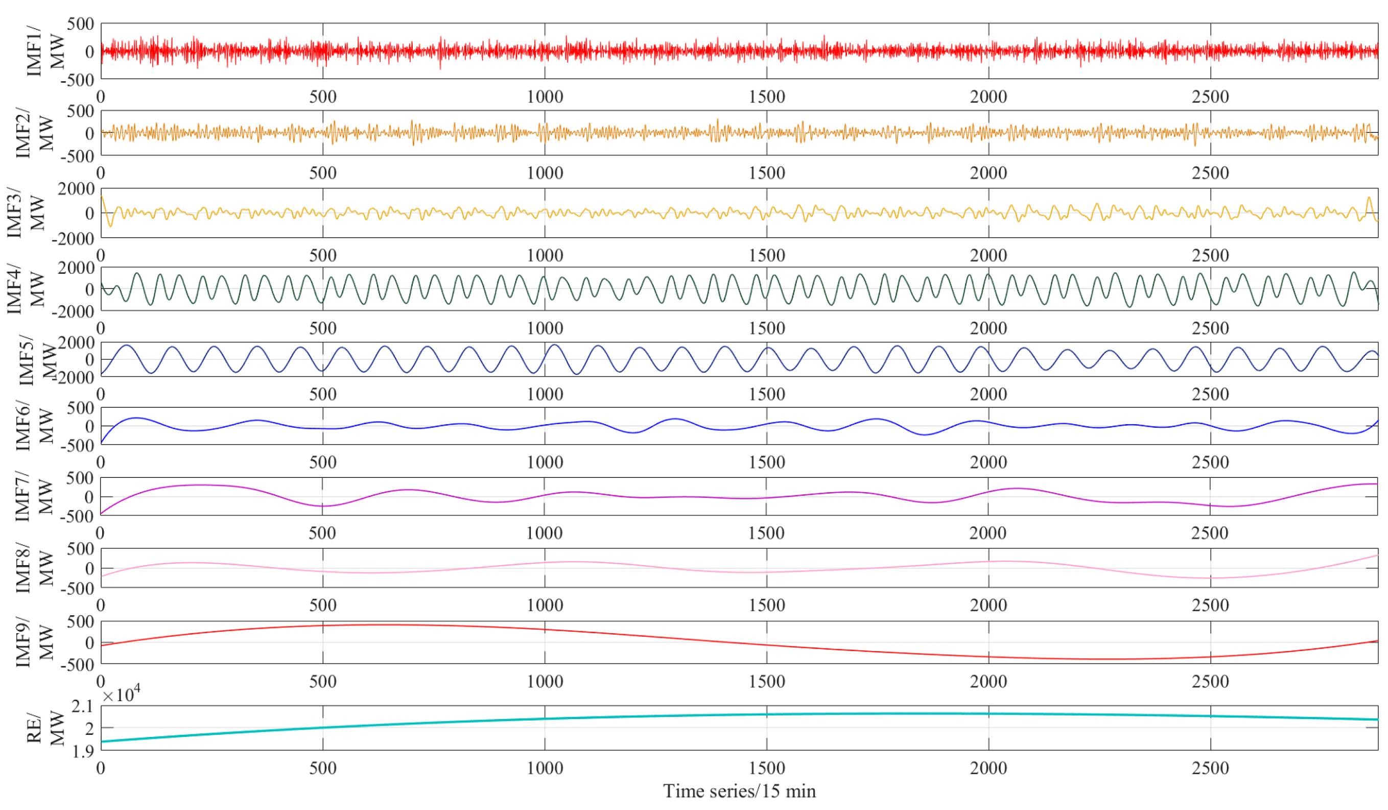
5.2. Load Sequence Decomposition Using AMD

The effectiveness of power load components extracted by AMD plays an important role in load forecasting. Based on some relevant research, the decomposition number of AMD is set from 4 to 12. Then, the optimal decomposition number can be determined by obtaining the minimum energy loss. The change in energy loss of AMD under different decomposition numbers is displayed in Figure 3.

It can be seen from Figure 3 that different decomposition numbers have different energy loss, proving the importance of the decomposition number for AMD. For example, when the decomposition number is set to 4, the energy loss has the highest value, demonstrating that the load sequence cannot be effectively decomposed. On the other hand, when the decomposition number is over 9, the energy loss decreases, which demonstrates that the AMD may generate some spurious components. Thus, the optimal decomposition number is set to 9 for achieving minimum energy loss. Then, the power load sequence is decomposed by AMD and the decomposition result is displayed in Figure 4.

As shown in Figure 4, the raw power load sequence is decomposed into nine different IMF components and a residual component. These load components contain multiple-frequency information and can provide more load detail, which can effectively improve the feature representation power.

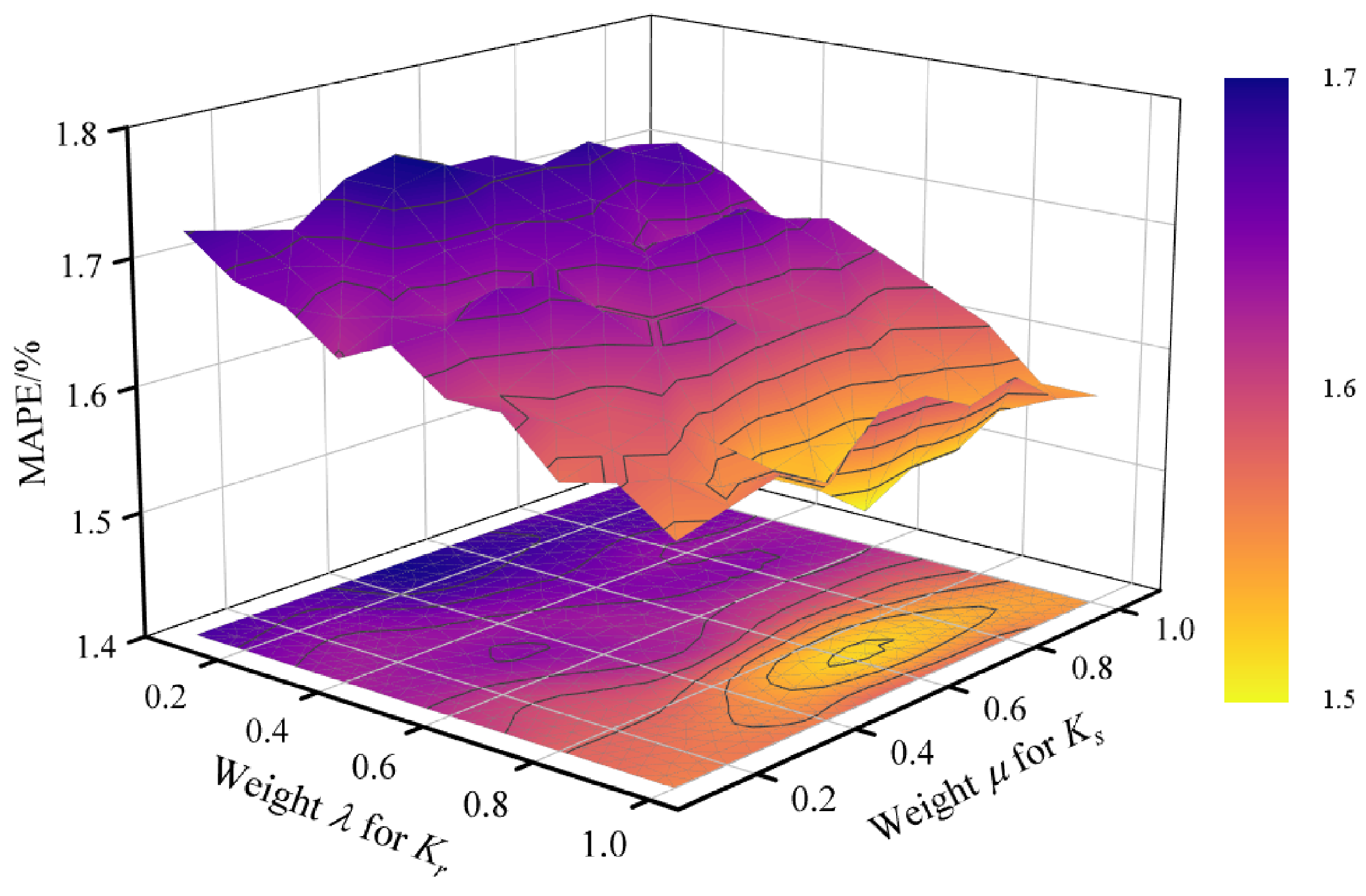
5.3. Parameter Selection for ILSSVM

Based on the load components provided by AMD, the ILSSVM is utilized to forecast different load components. In ILSSVM, kernel weights ($\lambda$, $\mu$) and kernel parameters ($\sigma$, $\theta$) directly affect the forecasting performance. In this research, the MAPE is selected as the evaluation metric of forecasting performance. To intuitively display the effects of model parameters, take the IMF4 as an example; the forecasting performance change in ILSSVM under different kernel weights is shown in Figure 5.

The step sizes for both $\lambda$ and $\mu$ are set to 0.1. It can be seen from Figure 5 that these two kernel weights affect the forecasting performance of ILSSVM for IMF4. The kernel weight $\lambda$ for the RBF kernel has a higher value when the MAPE reaches the lowest, indicating the combination kernel emphasizes the learning capability to obtain more detail information of IMF4. Additionally, the weight $\mu$ for the sigmoid kernel still retains some proportion, which can contribute to improve the generalization capability of the RBF kernel.

Then, the OGA is utilized to provide more accurate kernel weights; additionally, the other two kernel parameters $\sigma$ and $\theta$ are searched at the same time. The specific parameter settings of ILSSVM for different load components are listed in

Table 1. Parameters of ILSSVM for different load components.

Load Components	Model Parameter
	$\mathbf{\lambda }$	$\mathbf{\mu }$	$\mathbf{\sigma }$	$\mathbf{\theta }$
IMF1	0.91	0.59	0.77	−0.24
IMF2	0.87	0.44	0.68	−0.33
IMF3	0.89	0.57	0.84	−0.41
IMF4	0.92	0.61	0.58	−0.15
IMF5	0.81	0.35	0.82	−0.29
IMF6	0.72	0.56	0.59	−0.84
IMF7	0.68	0.64	1.09	−0.95
IMF8	0.60	0.42	0.98	−0.74
IMF9	0.80	0.68	0.59	−0.62
RE	0.64	0.39	0.72	−0.54

. From Table 1, it shows that the weights assigned to RBF and sigmoid are different for different load components, which indicates an adjustment and balance of learning capacity and generalization capacity for each unique load component.

5.4. Verification for the AMD

To validate the proposed AMD method, some popular decomposition including EMD [25], VMD [24], and EEMD are selected as a comparison. These signal decomposition methods are combined with the ILSSVM model for fair comparison. To distinguish the EEMD and AMD, the decomposition in EEMD is set to 8, which is an empirical value for load forecasting. The experimental results are listed in

Table 2. Performance comparison under different signal decomposition methods.

Combination Model	MAPE (%)
EMD with ILSSVM	2.02
VMD with ILSSVM	1.90
EEMD with ILSSVM	1.86
AMD with ILSSVM	1.78

.

It can be seen from Table 2 that the ILSSVM has different MAPEs, proving that the suitable signal decomposition process is highly important for accurate STLF. For example, the EEMD with ILSSVM has a lower MAPE than the EMD with ILSSVM, which shows that the mode mixing and end effect will decrease the effectiveness of load components provided by EMD. The EEMD can help to address the drawback of EMD, thus, the EEMD with ILSSVM has a better forecasting performance. Moreover, the proposed AMD with ILSSVM obtains the lowest MAPE of 1.78%, proving that the adaptive decomposition strategy based on minimum energy loss can provide more effective detail information and is more suitable for STLF.

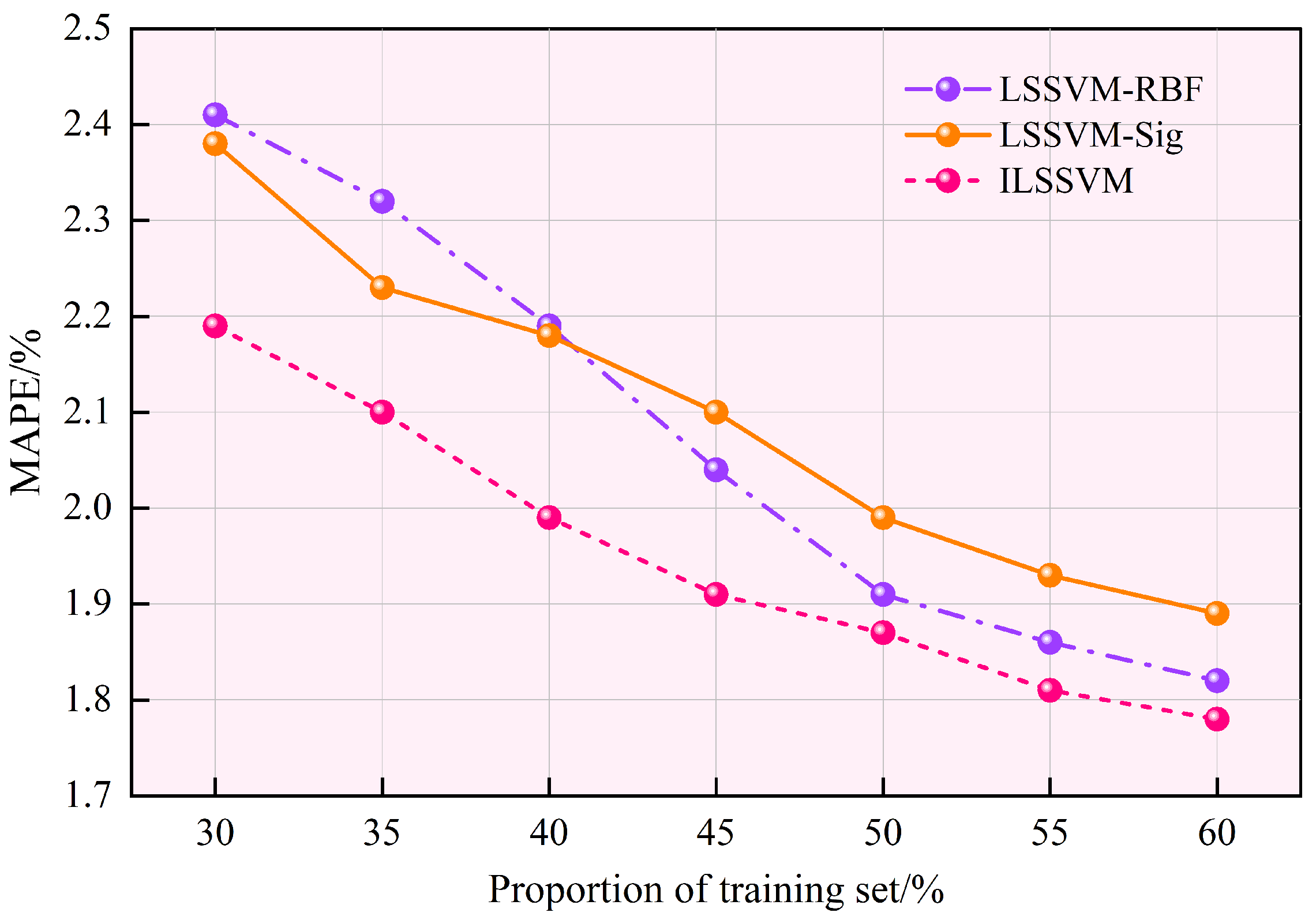
5.5. Verification for ILSSVM

To verify the effectiveness of the proposed ILSSVM, we first compare the ILSSVM with some popular single-kernel structures including RBF kernel (LSSVM-RBF) and sigmoid kernel (LSSVM-Sig). To provide a fair comparison, these LSSVM models are combined with AMD and their parameters are all optimized by the OGA. Additionally, the proportion of the training set is also considered to verify model robustness. The comparison result is presented in Figure 6.

From Figure 6, it shows that the training data has an important impact for these LSSVM models. When the proportion of training set ranges from 30% to 60% with the step size of 5%, the forecasting performances of these LSSVM models improve with the increase in the proportion of training set, indicating more effective load information is utilized. The proposed ILSSVM achieves the lowest MAPE across varying proportions of training data, which demonstrates superior robustness and forecasting accuracy. It proves that the combination kernel can effectively balance the learning capacity of the RBF kernel and generalization capacity of the sigmoid kernel for each unique load component, validating its effectiveness.

Moreover, some advanced optimization methods are used to validate the OGA including simulated annealing (SA), multiple adaptive genetic algorithm (MAGA) [31], and improved particle swarm optimization (IPSO) [32]. These optimization methods are used to adjust the parameters of ILSSVM and the MAPE of the corresponding forecasting model and can be utilized to reflect the optimization performance. The experimental results are given in

Table 3. Performance comparison under different parameter optimization methods.

Combination Model	MAPE (%)
ILSSVM with SA	1.93
ILSSVM with MAGA	1.85
ILSSVM with IPSO	1.82
ILSSVM with OGA	1.78

.

From Table 3, it shows that the IPSO and MAGA outperform the SA in this research. The MAPE of ILSSVM with SA is 1.93% while those of ILSSVM with MAGA and ILSSVM with IPSO are 1.85% and 1.82%, respectively. This result shows that the traditional SA finds it difficult to balance the global performance and local performance. By integrating the AGA and SA, the proposed OGA achieves the lowest MAPE, proving its superiority for parameter optimization of ILSSVM.

5.6. STLF Method Comparison and Discussion

To further verify the proposed STLF framework based on AMD and ILSSVM, some other STLF methods are selected for comparative analysis including ARIMA [33], ANN [18], LSTM [25], and CNN-LSTM [34]. The comparison results are listed in

Table 4. Performance comparison with other STLF methods.

STLF Model	MAPE (%)
ARIMA	3.82
ANN	2.93
LSTM	2.26
CNN-LSTM	1.89
the proposed framework	1.78

.

From Table 4, the LSTM and CNN-LSTM outperform the ARIMA and ANN in this research. The ARIMA has the highest MAPE, which shows that the ARIMA has difficulty accurately tracking the non-stationary and nonlinear characteristics of power loads. The CNN-LSTM is a bit better than LSTM. The MAPE of CNN-LSTM is 1.89%, while that of LSTM is 2.26%, indicating the combination structure can improve the effectiveness of load information to enhance the forecasting performance. It can be seen that the proposed STLF framework achieves the lowest MAPE, proving the load sequences inherently contain non-stationary components separable via AMD and the decomposed subseries can be effectively modeled by our ILSSVM, validating the forecasting performance of the proposed combination of AMD and ILSSVM.

6. Conclusions

In this article, a hybrid framework based on AMD and ILSSVM was proposed for short-term power load forecasting. Multiple power load components could be effectively extracted and analyzed using the proposed AMD method, where the decomposition number could be reasonably given based on minimum energy loss. In the load forecasting stage, the ILSSVM was proposed to significantly improve the forecasting performance by using a combination kernel structure and OGA. Extensive experiments were carried out and the results demonstrated that the proposed framework had strong robustness and accuracy for short-term power load forecasting. Built upon the forecasting result, this research could help to improve operational efficiency of the power system and reduce power generation costs.

The weaknesses and limitations include that the proposed framework has a high dependency on historical load data quality, as AMD decomposition may underperform in emerging grids with sparse operational records. Additionally, the combined effect of external factors such as extreme weather events is limited. Future research will focus on constructing a multi-modal forecasting framework that fuses spatiotemporal correlations and renewable generation dynamics.

References

1. Chen, Z.; Du, C.; Zhang, B.; Yang, C.; Gui, W. A Cybersecure Distribution-Free Learning Model for Interval Forecasting of Power Load Under Cyberattacks. IEEE Trans. Ind. Inform. 2025, 21, 2540–2549. [Google Scholar] [CrossRef]
2. Xiao, J.W.; Cui, X.Y.; Liu, X.K.; Fang, H.; Li, P.C. Improved 3-D LSTM: A Video Prediction Approach to Long Sequence Load Forecasting. IEEE Trans. Smart Grid 2025, 16, 1885–1896. [Google Scholar] [CrossRef]
3. Timur, O.; Üstünel, H.Y. Short-Term Electric Load Forecasting for an Industrial Plant Using Machine Learning-Based Algorithms. Energies 2025, 18, 1144. [Google Scholar] [CrossRef]
4. Jiang, B.; Wang, Y.; Wang, Q.; Geng, H. A Novel Interpretable Short-Term Load Forecasting Method Based on Kolmogorov-Arnold Networks. IEEE Trans. Power Syst. 2025, 40, 1180–1183. [Google Scholar] [CrossRef]
5. Pramanik, A.S.; Sepasi, S.; Nguyen, T.L.; Roose, L. An ensemble-based approach for short-term load forecasting for buildings with high proportion of renewable energy sources. Energy Build. 2024, 308, 113996. [Google Scholar] [CrossRef]
6. Mokarram, M.J.; Rashiditabar, R.; Gitizadeh, M.; Aghaei, J. Net-load forecasting of renewable energy systems using multi-input LSTM fuzzy and discrete wavelet transform. Energy 2023, 275, 127425. [Google Scholar] [CrossRef]
7. Akhtar, S.; Shahzad, S.; Zaheer, A.; Ullah, H.S.; Kilic, H.; Gono, R.; Jasiński, M.; Leonowicz, Z. Short-Term Load Forecasting Models: A Review of Challenges, Progress, and the Road Ahead. Energies 2023, 16, 4060. [Google Scholar] [CrossRef]
8. Tang, Y.; Cai, H. Short-Term Power Load Forecasting Based on VMD-Pyraformer-Adan. IEEE Access 2023, 11, 61958–61967. [Google Scholar] [CrossRef]
9. Shi, J.; Zhong, J.; Zhang, Y.; Xiao, B.; Xiao, L.; Zheng, Y. A dual attention LSTM lightweight model based on exponential smoothing for remaining useful life prediction. Reliab. Eng. Syst. Saf. 2024, 243, 109821. [Google Scholar] [CrossRef]
10. Zhong, W.; Zhai, D.; Xu, W.; Gong, W.; Yan, C.; Zhang, Y.; Qi, L. Accurate and efficient daily carbon emission forecasting based on improved ARIMA. Appl. Energy 2024, 376, 124232. [Google Scholar] [CrossRef]
11. Song, H.; Xia, J.; Hu, Q.; Cheng, W.; Yang, Y.; Chen, H.; Yang, H. Comprehensive experimental assessment of biomass steam gasification with different types: Correlation and multiple linear regression analysis with feedstock characteristics. Renew. Energy 2024, 237, 121649. [Google Scholar] [CrossRef]
12. Wan, A.; Chang, Q.; AL-Bukhaiti, K.; He, J. Short-term power load forecasting for combined heat and power using CNN-LSTM enhanced by attention mechanism. Energy 2023, 282, 128274. [Google Scholar] [CrossRef]
13. Fotis, G.; Vita, V.; Ekonomou, L. Machine Learning Techniques for the Prediction of the Magnetic and Electric Field of Electrostatic Discharges. Electronics 2022, 11, 1858. [Google Scholar] [CrossRef]
14. Sirsat, M.S.; Isla-Cernadas, D.; Cernadas, E.; Fernández-Delgado, M. Machine and deep learning for the prediction of nutrient deficiency in wheat leaf images. Knowl.-Based Syst. 2025, 317, 113400. [Google Scholar] [CrossRef]
15. Ma, K.; Nie, X.; Yang, J.; Zha, L.; Li, G.; Li, H. A power load forecasting method in port based on VMD-ICSS-hybrid neural network. Appl. Energy 2025, 377, 124246. [Google Scholar] [CrossRef]
16. Qu, K.; Si, G.; Shan, Z.; Wang, Q.; Liu, X.; Yang, C. Forwardformer: Efficient Transformer With Multi-Scale Forward Self-Attention for Day-Ahead Load Forecasting. IEEE Trans. Power Syst. 2024, 39, 1421–1433. [Google Scholar] [CrossRef]
17. Li, K.; Mu, Y.; Yang, F.; Wang, H.; Yan, Y.; Zhang, C. A novel short-term multi-energy load forecasting method for integrated energy system based on feature separation-fusion technology and improved CNN. Appl. Energy 2023, 351, 121823. [Google Scholar] [CrossRef]
18. Pajić, Z.; Janković, Z.; Selakov, A. Autoencoder-Driven Training Data Selection Based on Hidden Features for Improved Accuracy of ANN Short-Term Load Forecasting in ADMS. Energies 2024, 17, 5183. [Google Scholar] [CrossRef]
19. Dong, J.; Luo, L.; Lu, Y.; Zhang, Q. A Parallel Short-Term Power Load Forecasting Method Considering High-Level Elastic Loads. IEEE Trans. Instrum. Meas. 2023, 72, 1–10. [Google Scholar] [CrossRef]
20. Guo, W.; Liu, S.; Weng, L.; Liang, X. Power Grid Load Forecasting Using a CNN-LSTM Network Based on a Multi-Modal Attention Mechanism. Appl. Sci. 2025, 15, 2435. [Google Scholar] [CrossRef]
21. Wang, A.; Qin, P.; Sun, X.M.; Li, Y. An Automatic Parameter Setting Variational Mode Decomposition Method for Vibration Signals. IEEE Trans. Ind. Inform. 2024, 20, 2053–2062. [Google Scholar] [CrossRef]
22. Li, Y.; Zhou, J.; Li, H.; Meng, G.; Bian, J. A Fast and Adaptive Empirical Mode Decomposition Method and Its Application in Rolling Bearing Fault Diagnosis. IEEE Sens. J. 2023, 23, 567–576. [Google Scholar] [CrossRef]
23. Li, M.; Li, Y.; Choi, S.S. Dispatch Planning of a Wide-Area Wind Power-Energy Storage Scheme Based on Ensemble Empirical Mode Decomposition Technique. IEEE Trans. Sustain. Energy 2021, 12, 1275–1288. [Google Scholar] [CrossRef]
24. Wen, M.; Liu, B.; Zhong, H.; Yu, Z.; Chen, C.; Yang, X.; Dai, X.; Chen, L. Short-Term Power Load Forecasting Method Based on Improved Sparrow Search Algorithm, Variational Mode Decomposition, and Bidirectional Long Short-Term Memory Neural Network. Energies 2024, 17, 5280. [Google Scholar] [CrossRef]
25. Yin, C.; Wei, N.; Wu, J.; Ruan, C.; Luo, X.; Zeng, F. An Empirical Mode Decomposition-Based Hybrid Model for Sub-Hourly Load Forecasting. Energies 2024, 17, 307. [Google Scholar] [CrossRef]
26. Gao, Y.; Jiang, J.; Pan, J.; Yuan, B.; Zhang, H.; Zhu, Q. Contrastive learning-based fuzzy support vector machine. Neurocomputing 2025, 637, 130101. [Google Scholar] [CrossRef]
27. Ge, Q.; Guo, C.; Jiang, H.; Lu, Z.; Yao, G.; Zhang, J.; Hua, Q. Industrial Power Load Forecasting Method Based on Reinforcement Learning and PSO-LSSVM. IEEE Trans. Cybern. 2022, 52, 1112–1124. [Google Scholar] [CrossRef]
28. Ji, S.; Zhang, L.; Wang, J.; Wei, T.; Li, J.; Ling, B.; Xu, J.; Wu, Z. Short-Term Power Load Forecasting Based on DPSO-LSSVM Model. IEEE Access 2025, 13, 32211–32224. [Google Scholar] [CrossRef]
29. Qu, L.; Liu, C.; Yang, T.; Sun, Y. Vital Sign Detection of FMCW Radar Based on Improved Adaptive Parameter Variational Mode Decomposition. IEEE Sens. J. 2023, 23, 25048–25060. [Google Scholar] [CrossRef]
30. Ma, J.; Teng, Z.; Tang, Q.; Guo, Z.; Kang, L.; Wang, Q.; Li, N.; Peretto, L. A Novel Multisource Feature Fusion Framework for Measurement Error Prediction of Smart Electricity Meters. IEEE Sens. J. 2023, 23, 19571–19581. [Google Scholar] [CrossRef]
31. Ma, L.; Meng, Z.; Teng, Z.; Tang, Q. A measurement error prediction framework for smart meters under extreme natural environment stresses. Electr. Power Syst. Res. 2023, 218, 109192. [Google Scholar] [CrossRef]
32. Ge, L.; Li, Y.; Yan, J.; Wang, Y.; Zhang, N. Short-term Load Prediction of Integrated Energy System with Wavelet Neural Network Model Based on Improved Particle Swarm Optimization and Chaos Optimization Algorithm. J. Mod. Power Syst. Clean Energy 2021, 9, 1490–1499. [Google Scholar] [CrossRef]
33. Yan, S.; Hu, M. A Multi-Stage Planning Method for Distribution Networks Based on ARIMA with Error Gradient Sampling for Source–Load Prediction. Sensors 2022, 22, 8403. [Google Scholar] [CrossRef]
34. Al-Ja’afreh, M.A.A.; Mokryani, G.; Amjad, B. An enhanced CNN-LSTM based multi-stage framework for PV and load short-term forecasting: DSO scenarios. Energy Rep. 2023, 10, 1387–1408. [Google Scholar] [CrossRef]
Figure 2. Power load sequence of November 2022 of Guangxi region in China.
Energies 18 02491 g002
Figure 3. Energy loss of AMD under different decomposition numbers.
Energies 18 02491 g003
Figure 4. Load decomposition result of AMD.
Energies 18 02491 g004
Figure 5. Performance of ILSSVM under different kernel weights.
Energies 18 02491 g005
Figure 6. Performance comparison of LSSVM with different kernel structures under different proportions of training data.
Energies 18 02491 g006