A Spatial Long-Term Load Forecast Using a Multiple Delineated Machine Learning Approach

Abstract

Maintaining a balance between electricity generation and consumption is vital for ensuring grid stability and preventing disruptions. Spatial load forecasting (SLF) predicts geographical electricity demand, thereby aiding in power system planning. However, conventional methods like multiple linear regression and autoregressive integrated moving average struggle to capture the complex spatiotemporal patterns in historical data. Advanced methods like spatiotemporal graph transformers, graph convolutional networks, and improved scale-limited dynamic time warping better capture these dependencies, thereby enhancing prediction accuracy. Despite the advancements, challenges persist, particularly in developing economies with limited reliable data. This paper presents a novel SLF approach that divides the grid into predefined clusters based on regional characteristics and economic activity. For each cluster, a customized long short-term memory (LSTM) model captures unique spatiotemporal dependencies for more accurate predictions. The proposed method was tested across five load clusters using real-world data from Cameroon’s National Electricity Transmission Company and Energy Utilities. The results, compared against a linear regression model, demonstrated the superior performance of the LSTM approach across metrics like the mean absolute percentage error, root-mean-square error, mean absolute error, and R² score. This approach highlights the potential for enhanced, localized load forecasting in regions with data constraints.

1. Introduction

The power system serves as a foundation in modern society, underpinning economic growth, industrial development, and the overall quality of life. Electricity is indispensable for powering industries, infrastructure, and households, making it a critical resource for societal progress. However, managing the delicate balance between generation and consumption remains a major challenge. Unlike other commodities, electricity cannot be economically stored in large quantities; therefore, a real-time equilibrium is required to ensure grid stability, prevent blackouts, and optimize resources. Spatial load forecasting (SLF) helps to address this challenge by predicting electricity demand distribution across different regions. Accurate SLF helps utilities to anticipate future needs, guiding network expansion, substation reinforcement, and infrastructure planning. With the rapid urbanization and economic development in Cameroon, power loads are becoming increasingly dynamic, highlighting the importance of precise forecasting to maintain grid reliability [1]. These power load fluctuations must be captured, anticipated, and considered in network expansion planning [2]. A long-term forecast was proposed for the Southern Grid of Cameroon with an hourly timestep as a lump or global value. While insightful, this approach did not account for spatial (region-specific) variations, which are crucial for transmission and distribution planning. Understanding the precise amount of electricity required and its distribution is crucial for utilities to efficiently manage power flow, upgrade infrastructure, and configure systems. Therefore, this study aimed to develop a forecasting model to predict load magnitudes within various load clusters identified by distinct regions. This approach provides a more granular and region-specific view of future electricity demand, enabling more precise infrastructure development and policy decision-making.

SLF is defined as the spatial distribution of load with respect to the forecast horizon that could be differentiated into two primary categories: short-term and long-term SLF [3,4]. SLF is increasingly vital for the planning and management of modern electrical grids, particularly in developing economies that are still faced with severe disruptions and outages resulting from poor visibility of load evolution. The prediction of both the quantity and geographical distribution of electricity demand is imperative. The methods utilized vary from trending through simulation bases to even hybrid models. Recent studies primarily focused on simulation-based models. The authors of [5] presented a method to predict the geographical distribution of future electrical loads using a cellular automaton model, the utility’s long-term forecast, and a map of the study region. A hierarchical bottom-up load-accumulating approach utilized based on clustered typical load profiles was proposed, leveraging new data sources [6]. Furthermore, multiple hybrid models, such as stacked long short-term memory (LSTM) with convolutional neural networks (CNNs) and a hybrid deep learning method with and without skip connections, with enhanced accuracy were utilized [7]. This strives for the use of minimal data since data accumulation is a significant concern in load forecasting methodologies [8]. Different methods are suitable for large areas and long-term forecasting. A qualitative macroeconomic approach is used to determine load centers and power transmission directions [4]. Furthermore, GIS-based methods have provided somewhat satisfactory results [9,10].

Recent advancements in modeling techniques have significantly improved the spatial precision of demand forecasts. Recent studies have adopted the power of graph neural networks (GNNs) and deep learning as more intelligent models to better capture spatial and temporal trends in electricity demand. For example, the multi-scale spatial–temporal graph neural network (MS-STGNN) was introduced [11]. This approach utilizes continuous graph learning to dynamically quantify relationships between features and applies a multi-scale temporal convolution to extract features across various time scales, resulting in enhanced spatial clustering and improved prediction accuracy. Similarly, this novel modeling approach was further supported in a previous study [12]. Despite the predictive accuracy attained, a key limitation is its computational complexity, which may hinder real-time applications or large-scale deployments. These approaches allow utilities to effectively distribute resources, particularly in urban centers. However, its performance significantly depends on high-quality spatial data and can degrade in less densely monitored regions. Researchers also focused on the utilization of transformer models in predicting energy. Transformers, originally designed for natural language processing, are currently being leveraged in spatial energy forecasting. A novel spatiotemporal dynamic graph transformer (SDGT), which integrates a multi-scale transformer module with a patch-based multi-scale encoder to capture multiple periodic patterns and extract temporal dependencies was proposed [13]. These methods offer a nuanced understanding of energy consumption patterns, aiding in preventing overloading and enhancing grid stability. Further research in SLF has progressed toward convolution-based methods (newer), leveraging a neighborhood influence to simulate load diffusion, thereby allowing forecasts even in previously unoccupied regions. These methods paved the way for the convolutional spatial model proposed in [14], which explicitly incorporated attraction poles, constraint areas, and local growth dynamics in a computationally efficient manner. Most of these methods require a significant amount of data. However, owing to the challenges in acquiring such data, a discrete model with reduced data utilization was developed [5], making it suitable for emerging economies. However, no standardized benchmark system has been established to compare the results of this method with those obtained through other methodologies, rendering it challenging to comprehensively validate the model’s accuracy and effectiveness. Recent advancements in SLF emphasize the integration of georeferenced information and computational intelligence tools to improve investment decisions and enhance power system planning and network expansion [15]. Utilities must focus on realistic data requirements and practical visualization techniques to enhance the adoption of SLF methods [16].

Cameroon’s Southern Grid encompasses the country’s major load centers and has been structured into three primary electric regions by the National Transmission Utility, SONATREL, to optimize grid operations, as follows: Littoral-Southwest (over 50% of the total load), Center-Southeast (35% of the total load), and Western (15% of the total). To enhance the accuracy of SLF, this study refines these three broad regions into five distinct clusters—South, Southwest, Littoral, Center, and West–Northwest—which align with the administrative divisions of the Southern Grid [4]. Our method entails forecasting loads within these respective regions, thereby providing a tool for the forecasting of future loads through machine learning techniques. This study uses a reduced set of data for a long-term SLF model (multiple LSTM cluster model). The load curves in these regions enable the visualization of the spatial distribution of the load density, which will allow SONATREL to plan for its network expansion since it considers both load magnitude variation and location distribution information of each region.

The remainder of this paper is organized as follows: Section 2 outlines the methodology and materials utilized. The results are presented in Section 3. Finally, the key conclusions are summarized in Section 4.

2. Materials and Methods

This study utilizes multivariate input sequences comprising historical load data, demographic trends, socioeconomic variables (economic growth), and temporal factors (hour of the day, day of the week, and month of the year) as the ground truth for 2006–2016. To forecast for 2016–2020, the dataset integrates projected population growth and economic activity indicators, along with the same temporal variables. A supervised machine learning model specifically designed for regression tasks is developed and trained using these multivariate input data to predict future load demands.

2.1. Data Acquisition, Processing, and Segmentation

Economic load centers, also referred to as load clusters, are crucial in SLF. In Cameroon, these centers typically correspond to the capital cities of each administrative region as they are key hubs of economic activity. Prior research [4] has demonstrated that defining spatial units based on economic growth enhances the effectiveness of transmission planning. The authors propose a qualitative approach that associates electricity demand forecasting with economic growth centers rather than just land use patterns. In this study, we segment the forecast area (the Southern Grid also known as the RIS) into five clusters, which align with the economic growth centers of Cameroon where the study is conducted: South (SO), Southwest (SW), Littoral (LT), Center (CE), and West–Northwest (WN). This clustering approach facilitates a localized and region-specific forecasting framework, ensuring that the electricity demand forecast accurately reflects the economic and demographic dynamics of each area. The decision to partition the Cameroonian Southern Interconnected Network (RIS) into five clusters or regions—Littoral, Center, West–Northwest, Southwest, and South—results from a deliberate analysis combining scientific criteria for power system zoning and specific characteristics of the national grid. The analysis for clustering was based on the following.

-

Electrical and Topological Coherence

Clustering was guided by the principle of strong intra-cluster connectivity and weak inter-cluster coupling, as suggested in power system community detection methods. The Littoral cluster is characterized by a dense 90 kV meshed grid linking cities with short transmission distances and strong mutual coupling. In contrast, the South and West–Northwest zones are separated by long radial lines (e.g., 225 kV Bekoko–Tchouwong–Bafoussam–Bamenda, or Ebolowa–Mbalmayo) with relatively low power exchanges under normal operation, making them electrically distinct. This ensures that each cluster forms a quasi-autonomous subsystem, minimizing prediction noise caused by external interactions and allowing for localized load behavior to be better captured.

-

Geographical and Climatic Homogeneity

Electrical demand is closely correlated with geographical factors, such as:

• Climate zones (e.g., humid tropical coast versus temperate highlands);
• Altitude (lowland LT versus elevated WN);
• Urban density and land use (dense commercial centers versus rural peripheries).

The defined clusters properly align with these physical–geographic partitions: The Center cluster (Yaoundé and surroundings) has homogeneous climatic conditions and demand patterns distinct from the SW or WN.

-

Socioeconomic Load Typology

Different clusters demonstrate fundamentally distinct load consumption profiles. The Littoral and Southwest zones are marked by industrial and port-driven demand (e.g., aluminum smelters, oil refineries, cement factories, and seaports). The Center cluster is driven by residential and governmental loads, whereas the Northwest and West zone feature dispersed, semi-urban, and agricultural loads. These distinctions justify separate forecasting models per cluster, enabling each to learn from consumption data with similar temporal dynamics (peak times, seasonality, and tariff responsiveness).

-

Operational Zoning and Contingency Management

The RIS already operates with an implicit zonal strategy for load shedding, voltage control, and reactive compensation. For example, in the event of a contingency in the South cluster, the long transmission distances (e.g., 225 kV Ebolowa–Memve’ele–Ahala line) and transformer bottlenecks isolate the zone from the rest of the system, justifying its independent treatment. Similarly, the Northwest and West zones have historically required islanded operation planning in low-voltage conditions. This operational separation supports the development of independent demand prediction models per cluster, aligning with actual grid management logic.

-

Generation–Load Balancing Characteristics

Each cluster contains at least one dispatchable generation facility (hydro or thermal) and a distinct generation–load ratio, influencing local balancing strategies. Examples include:

• South cluster: Large base-load capacity (KRIBI power plant, MEMVE’ELE hydropower plant) and low local demand, implying a potential net power exporter.
• Littoral cluster: Dense demand with moderate hydro generation, which implies, structurally, a net importer.
• West–Northwest cluster: Limited generation, high terrain-induced losses, implying that it could import capacity.

This heterogeneity supports the design of generation-aware forecasting models (e.g., incorporating local generation schedules, n-1 reserve margins). A summary of the clustering process is presented in

Table 1. Clusters based on the analyzed characteristics.

Clusters/Region	Analyzed Characteristics
Littoral Cluster	Includes major industrial and urban load centers, such as the city of Douala, the Edea–Songloulou, and the Kribi generation corridor. It is characterized by - Dense 90 kV mesh network; - High industrial demand (such as aluminum smelters, cement factories, and oil refineries); - Strong internal generation from hydro and thermal plants.
Center Cluster	Covers the city of Yaoundé metropolitan area and surrounding zones, including Kondengui, Nkolanga, Nsimalen, Oyomabang, and Ngousso. This area is marked by - Predominantly residential and administrative consumption; - Important nodes for voltage control and power injection; - Strategic centrality in national grid routing.
West-Northwest Cluster	Comprises highland nodes, such as Bafoussam, Bamenda, Dschang, and Nkongsamba. This region is characterized by - Dispersed loads across mountainous terrain; - Limited interconnectivity and longer radial transmission paths; - Greater sensitivity to local demand peaks and supply contingencies.
Southwest Cluster	Includes the cities of Limbe, Bekoko, Logbaba, and their adjacent industrial infrastructures. It is characterized by - High reliance on heavy fuel-based generation (Limbe power plant); - Strategic export/import potential via the Kribi–Mangombe corridor; - A dynamic interface between coastal and central zones.
South Cluster	Encompasses the cities of Ebolowa, Mbalmayo, and Memve’ele. It is - A zone of emerging generation capacity (hydro and thermal); - Key for future load growth and export potential; - Connected through long-range 225 kV corridors to the Center cluster.

.

Over the past decade, significant advancements have been made in the field of SLF. These advancements have involved the integration of various data sources such as geographic load distribution maps, economic indicators, and historical consumption patterns. To facilitate time-series forecasting, the continuous dataset is transformed into discrete sequential segments, ensuring a structured representation of load variations over time. The network region is divided into five distinct clusters, each corresponding to a specific administrative division of the grid. Each cluster maintains a dedicated multivariate dataset, allowing for region-specific forecasting and a more precise understanding of spatial load distribution.

While historical RIS load data were readily available for 2006–2024, regional load data corresponding to individual clusters were incomplete. To address this limitation, regional load distributions were derived by allocating the total RIS load proportionally across the different regions based on observed consumption patterns. The observed load consumption pattern was based on insufficient regional load data for the different clusters. This approach ensures a realistic and data-driven estimation of the regional electricity demand.

Based on these percentages, the previous RIS load data are split into five clusters that align with the aforementioned administrative regions in Figure 1.

Furthermore, owing to the unavailability of regional GDP data for the area under investigation, we used the name “economic growth” as a proxy for GDP per cluster because we needed to use the level and intensity of economic activity in a region as a surrogate indicator of the intensity of the region’s electricity consumption. This can be best captured by the regional GDP. However, the level and intensity of economic growth per cluster can also be a viable alternative. Economic growth per cluster is considered a weighted average of the GDP based on a repartition realized by the World Bank Group on Cameroon City Competitiveness Diagnostic [14]. The GDP data were obtained from the World Bank data on GDP of Cameroon for 2006–2020 for the entire nation, with a yearly timestep.

Demographic data were readily obtained from Cameroon’s National Institute of Statistics website. The data obtained have a quarterly timestep. We used them as hourly values, given that the population growth could not be captured at a lower level of granularity. Equally, in long-term forecasting, changes in the population growth within a short period were not sensitive to the model.

Table 2. Sample of the dataset for ground truths for LT

Datetime	Load (MW)	Population	Economic Growth
01/01/2006 00:00	157.05	2,682,633.82139541	0.829840510211798
01/01/2006 01:00	151.2	2,682,633.82139541	0.829840510211798
01/01/2006 02:00	143.55	2,682,633.82139541	0.829840510211798
01/01/2006 03:00	138.15	2,682,633.82139541	0.829840510211798
01/01/2006 04:00	131.4	2,682,633.82139541	0.829840510211798
01/01/2006 05:00	138.6	2,682,633.82139541	0.829840510211798
01/01/2006 06:00	127.8	2,682,633.82139541	0.829840510211798
01/01/2006 07:00	115.65	2,682,633.82139541	0.829840510211798
01/01/2006 08:00	112.5	2,682,633.82139541	0.829840510211798
01/01/2006 10:00	113.4	2,682,633.82139541	0.829840510211798
…	…	…	…

below shows a sample of the dataset for ground truths for the sub case of LT.

The sample from the segment dataset is a vector of previous timesteps that is used to predict a target vector (load) of future steps. We employed an hourly timestep for both the input and output horizons. Linear interpolation techniques were utilized to handle missing data and other anomalies, such as outliers. A robust estimation technique (M-estimation) was employed.

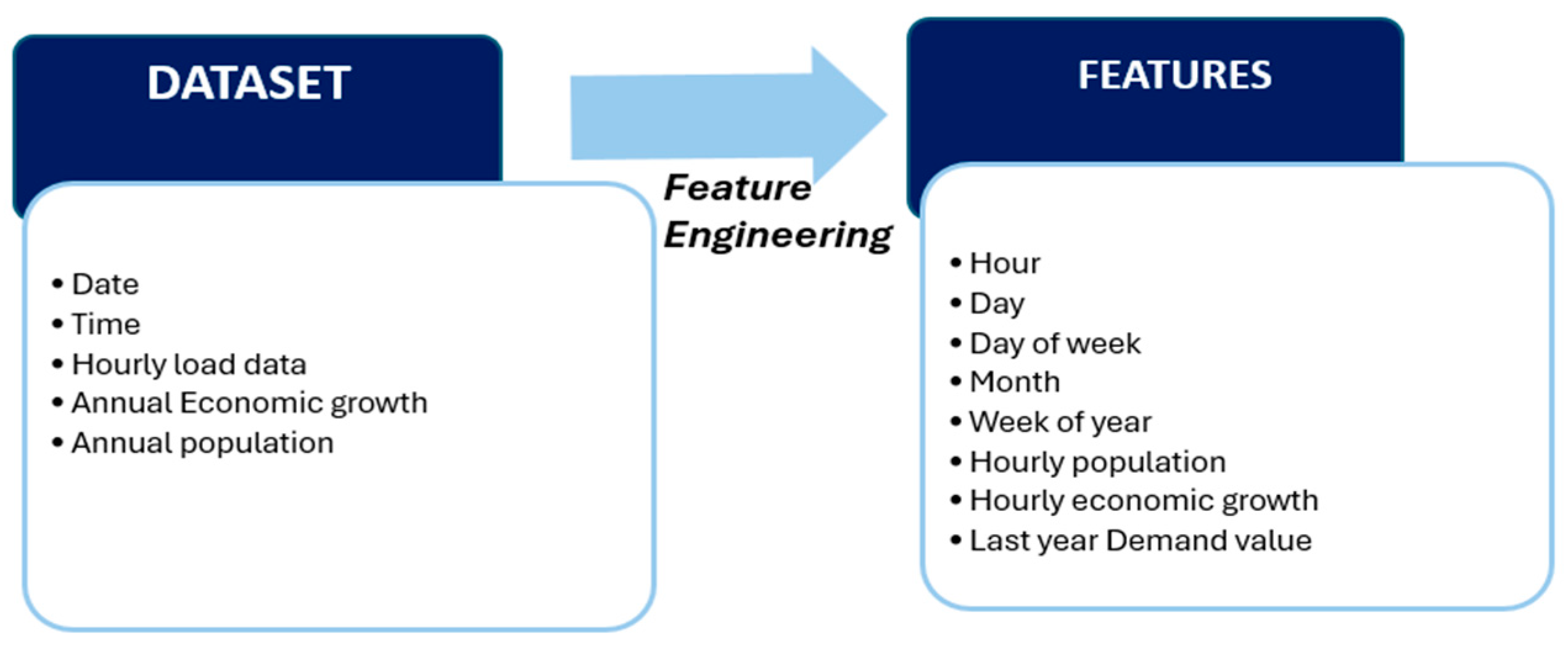
2.2. Feature Engineering

Many factors influence electricity consumption; however, for efficient model performance, the features should be determined from the dataset that influence the load demand and new features that may help improve the model performance should be developed. The step of feature engineering, which is crucial in the modeling process, is used to identify influencing factors. Data for the electricity demand were readily available hourly; however, it was not the case for the population and economic growth data. As a workaround, the economic growth and population data for each year were used for every hour of that year. The date and time were equally utilized as inputs to the neural network, but not in their original forms. First, they were converted to the corresponding hour, day of the week, month, and week of the year because these are important determinants of the electricity demand. For example, the electricity demand on Fridays (the fifth day of the business week) havhase a particular trend throughout the year and over many years. A similar remark can be made regarding other dates and time data. Furthermore, the cyclical nature of these date and time data must be reflected in the features. This indicates that the proximity of day 7 to day 1 and hour 24 to hour 1 should be evident in the feature. The load demand for the same day and hour of the previous year is the most important feature attributed to routine activities, and the weather conditions tend to be similar during the same period of each year in each region. However, the proposed model does not include weather parameters owing to the unpredictable nature of the climate over five years. This method employs cyclical feature encoding, which is based on trigonometry.

To address seasonality in our LSTM-based model, we derived additional cyclical features from the date and time features. Specifically, we extracted the hour of day, day of the week, month, and week of the year, and transformed them using sine and cosine functions to capture their periodic nature. This transformation ensures that cyclical endpoints are close in representation—for example, hour 23 and hour 0 were treated as adjacent, similar to hour 0 and hour 1. Similarly, Sunday (day 7) and Monday (day 1), December (month 12) and January (month 1), as well as week 52 and week 1, were treated as adjacent to Tuesday (day 2), February (Month 2), and week 2, respectively.

The sine and cosine transformations were performed using the following equations:

$$X_{\mathrm{c}\mathrm{y}\mathrm{c}\mathrm{l}\mathrm{i}\mathrm{c}\mathrm{a}\mathrm{l}}^{\mathrm{s}\mathrm{i}\mathrm{n}}=\sin \left(2\pi \cdot {\displaystyle \frac{X-X_{\mathrm{start} }}{X_{\mathrm{p}\mathrm{e}\mathrm{r}\mathrm{i}\mathrm{o}\mathrm{d}} }}\right),\mathrm{and} X_{\mathrm{c}\mathrm{y}\mathrm{c}\mathrm{l}\mathrm{i}\mathrm{c}\mathrm{a}\mathrm{l}}^{\mathrm{c}\mathrm{o}\mathrm{s}}=\cos \left(2\pi \cdot {\displaystyle \frac{X-X_{\mathrm{start} }}{X_{\mathrm{p}\mathrm{e}\mathrm{r}\mathrm{i}\mathrm{o}\mathrm{d}}}}\right)$$

(1)

where

• For hours of the day: $X_{\mathrm{start}}=0,\mathrm{a}\mathrm{n}\mathrm{d} X_{\mathrm{period}}=24$
• For days of the week: $X_{\mathrm{start}}=0,\mathrm{a}\mathrm{n}\mathrm{d} X_{\mathrm{period}}=7$
• For months: $X_{\mathrm{start}}=1,\mathrm{a}\mathrm{n}\mathrm{d} X_{\mathrm{period}}=12$
• For weeks of the year: $X_{\mathrm{start}}=0,\mathrm{a}\mathrm{n}\mathrm{d} X_{\mathrm{period}}=52$

As observed, the encoding outperforms conventional one-hot encoding in capturing cyclical patterns in temporal data, resulting in enhanced model generalization and forecasting performance [17].

Data pairs that include an hourly value as the output and data from the previous week (168 h) were used as the input for model training, validation, and testing. The handling of the features is shown in Figure 2. Notably, the training and test data must originate from the same distribution, thereby facilitating and expediting the training process. This was achieved by scaling the data using a min-max scaler [18] to ensure that the values are maintained within a certain range. With the demand of the previous year included as an input feature, our training data covered 2007–2014 (61,320 observations), whereas the validation data started from 2015 (8760 observations). Upon training and fine-tuning of the model based on the validation data, it was utilized to predict the load demand for 2016. This predicted load demand enables us to predict that for 2017. This process was performed until forecasts for 2016–2020 (5 years) were obtained. Therefore, our model can predict both short-term and long-term spatial loads.

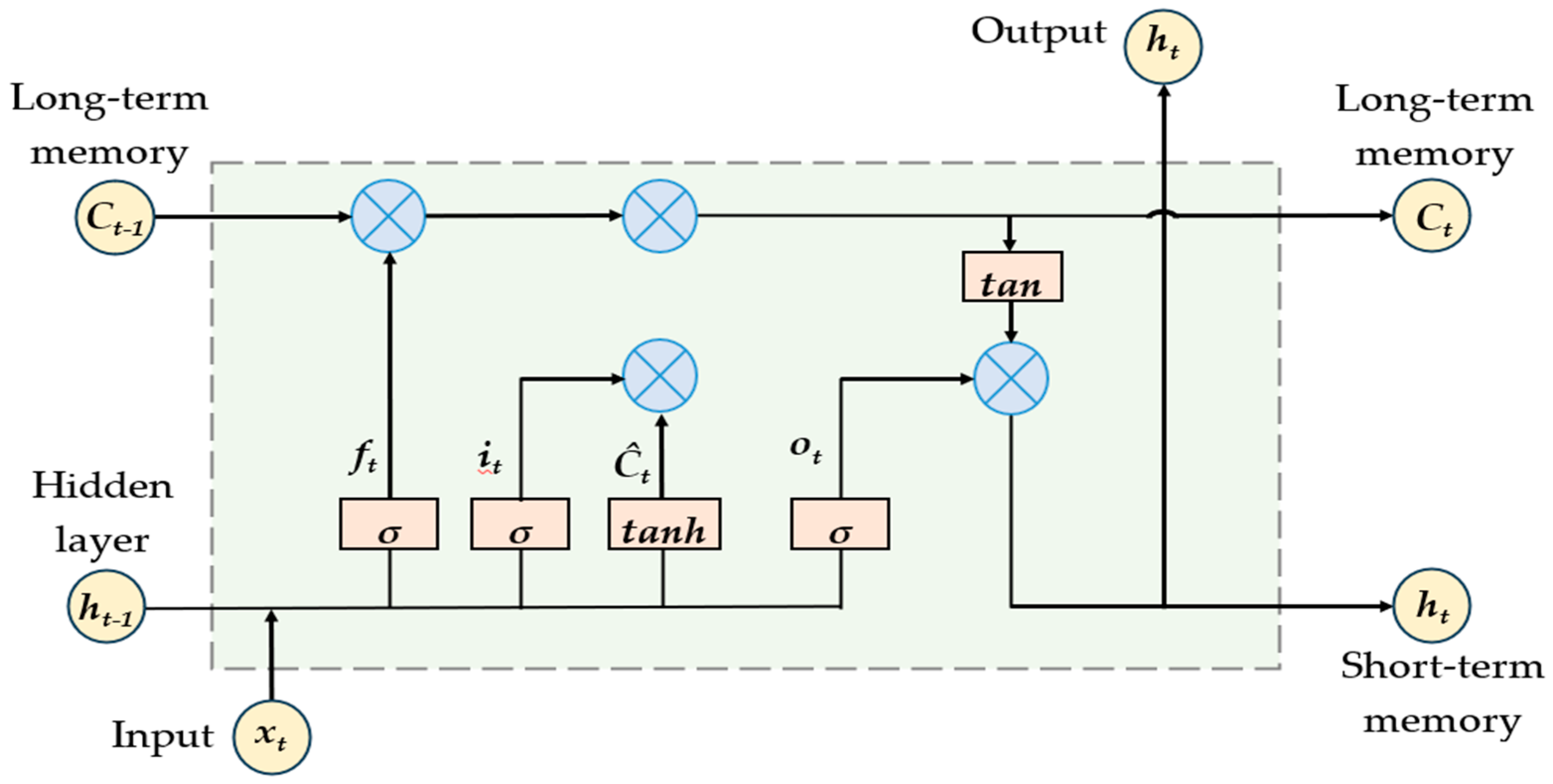
2.3. LSTM Neural Network

Long short-term memory (LSTM) neural networks, which are advanced forms of recurrent neural networks (RNNs), have emerged as a robust solution for time-series forecasting. Unlike conventional RNNs, LSTMs address the vanishing gradient problem, enabling them to retain long-term dependencies in sequential data. This makes them well-suited for modeling complex patterns and trends in electricity demand forecasting. LSTM models can learn both short-term fluctuations and long-term consumption patterns, making them highly suitable for forecasting electricity loads across different time scales, including real-time, short-term, medium-term, and long-term horizons. Owing to the nonlinear characteristics of the model parameters resulting from the interaction between the load and other variables, a model that can effectively capture this nonlinearity is required. This study addressed the issue by utilizing LSTM, which demonstrates superior performance in learning long-term time-series data. The use of LSTM facilitates a more effective learning of the long-term relationships in the data, allowing for a logical spatial prediction of a load that captures its nonlinearity. LSTM networks are based on the basic RNN by incorporating three special gates: the input, forget, and output gates. These gates help manage information flow through the network. Each unit in an LSTM can add or remove information, allowing it to determine what to maintain or discard at each step. This decision-making process involves a “gate” structure that utilizes a Sigmoid layer and vector multiplication to control data flow. The gates are crucial in overcoming some issues inherent in RNNs, such as vanishing and exploding gradients, which help the network learn more effectively and converge faster. The first step in the LSTM process is to determine the information to be discarded from the cell state. This is handled by the forget gate. The forget gate determines the parts of the cell state to be forgotten based on the current input and previous output. The forget gate utilizes a Sigmoid layer to transform the previous memory cell state Ct-1 and current input (t) into a value between 0 and 1. This value indicates the amount of information to be retained or discarded. The input gate has two components—a Sigmoid layer that decides whether to update the memory cell’s state and a tanh layer that generates a new candidate state for the memory cell. The output gate determines the value of the unit output. First, the Sigmoid layer is used to determine the parts of the state to output, followed by the application of the tanh function to scale the output (Figure 3).

2.4. Construction of LSTM Prediction Models

A supervised machine learning model specifically designed for regression tasks was utilized in this analysis. It was trained using historical load data to predict future load demands. The training process involved feeding the model with labeled data. The models are fed with hourly load data for the previous year, along with hourly population and economic growth data. These inputs help train the model to predict future loads for the respective clusters. Once trained, the model utilizes forecasted economic growth and population hourly data to predict system loads for the next five years. The model was trained and validated on the data on a rolling basis, and the predictions were made similarly. Predictions were made yearly and then appended to the training set, which was further employed to make predictions for the next year, and the process continues. Owing to the sequential nature of the dataset, we employed a sequence model, which can be considered an LSTM model owing to its excellent performance with time-series data. The linear unit (ReLU) was employed as the activation function for each layer. The best-performing model had three LSTM layers with an input size of 12 features, 168 (24 h for seven days) timesteps. The output sequence of each layer served as the input sequence of the next layer, comprising 64 features (neurons) in the hidden state. A dropout of 0.2 was applied to the outputs of each LSTM layer. The exit of the three LSTM layers featured a fully connected linear layer, which resulted in a single-dimensional output. The model was trained for 100 epochs, with each iteration in the epoch using a batch size of 64. The Adam optimizer was employed to train the model. The set of hyperparameters (resulting from an extensive hyperparameter tuning based on a grid search), when combined, provided the optimal convergence for our model during training. The Adam optimizer was utilized during training as it provides faster convergence, regardless of the sparsity of the gradient during training. Notably, more complex LSTM network combinations exist; however, for the scope of this work, the network architecture was constrained to maintain the space of hyperparameters at a minimum. This will be explored in future studies. The variation in loss during training is shown in Figure 4.

2.5. Evaluation Metrics

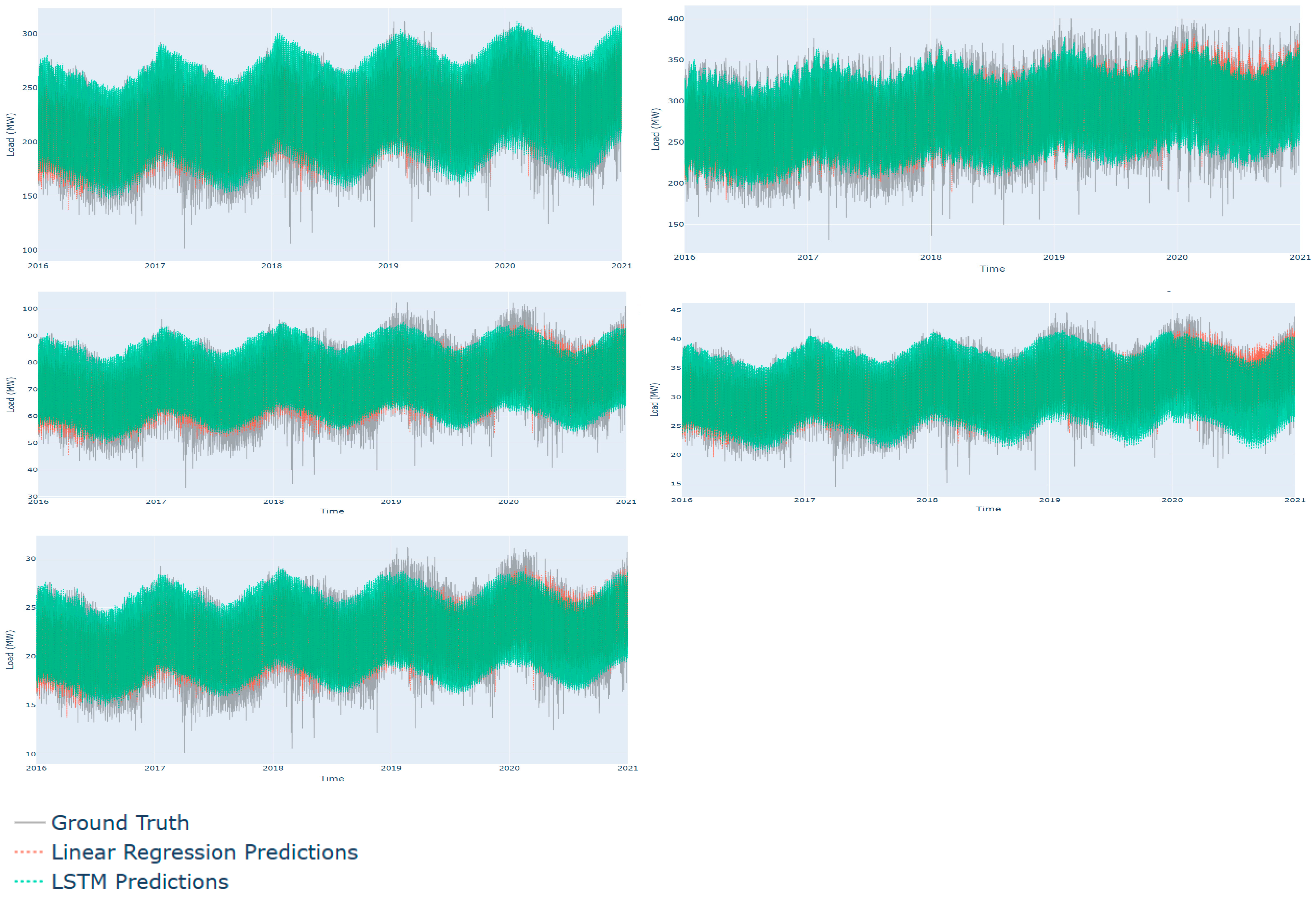
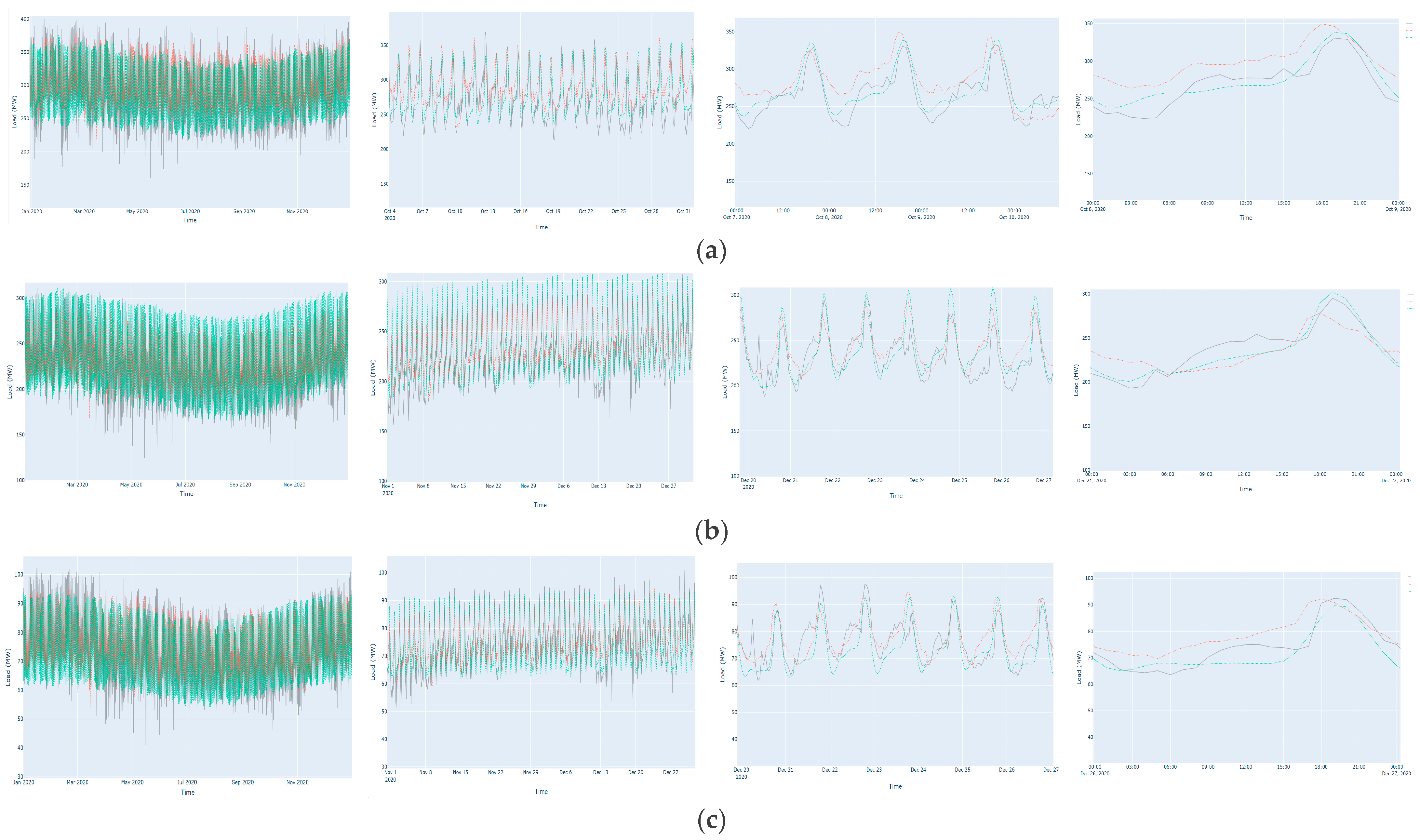
For model evaluation, we used the mean absolute percentage error (MAPE), mean absolute error (MAE), the root-mean-square residual (RMSR) and the R² score, evaluated as below.

$$MAPE={\displaystyle \frac{1}{n}}{\sum }_{t=1}^n\left|{\displaystyle \frac{A_t-F_t}{A_t}}\right|\ast 100\%$$

(2)

$$MAE={\displaystyle \frac{1}{n}}{\sum }_{t=1}^n\left|A_t-F_t\right|$$

(3)

$$RMSR=\sqrt{{\displaystyle \frac{1}{n}}\sum _{t=1}^n{\left(A_t-F_t\right)}^2}$$

(4)

$$R^2=1- {\displaystyle \frac{\sum _{t=1}^n{\left(A_t-F_t\right)}^2}{\sum _{t=1}^n{\left(A_t-\overline{A} \right)}^2}}$$

(5)

where n represents the number of observations, $A_t$ represents the actual value at time $t$, $F_t$ represents the forecasted value at time $t$, and $\overline{A}$ represents the mean of the actual values.

The evaluation metrics could be further extended to obtain confidence intervals. However, this process is more extensive in the case of deep neural networks (and typically involves changes to the model) and is beyond the scope of this work. The readership should refer to popular choices, such as the Monte Carlo dropout (MC dropout) [19,20], deep ensembles [21], quantile regression [22], Bayesian neural networks [23], and bootstrapping [24].

3. Results

This study utilizes the actual grid load from various regions as sample data for predictions. The dataset for each region or cluster was segmented into three portions: 86.5% for training, 3.5% for validation, and 10% for testing. Using this structured data, predictions were made employing both an LSTM prediction model and a linear regression (LR) model. Figure 5 presents the forecast results compared to the ground truth data for the five clusters over the period from 2016 to 2020. Additionally, Figure 6 provides a more detailed comparison of predicted versus actual load for selected time intervals: one year, one month, one week, and one day.

In our previous work [2], RIS hourly load data from 2006 to 2015 were employed to forecast system-wide load on a rolling basis for 2016–2020, covering the entire RIS area (denoted as RES00). In the current study, we utilized the same RIS hourly load data to approximate regional hourly load data (aReg) for 2006–2015, as the actual regional load data (rReg) were incomplete or unreliable for parts of that period. The rReg represents metered load measurements obtained at HV/MV substations across the different regions. Conceptually, the RIS load represents the aggregate of the loads from the five constituent regions. To estimate regional contributions, we compared rReg and RIS hourly load data for 2018–2020—when complete rReg time-series data were available—and obtained average regional percentage contributions relative to the total RIS load (Figure 1). Subsequently, these percentage values were applied to the RIS load data to estimate the aReg hourly load data for 2006–2017. The resulting aReg data for 2006–2015 were subsequently utilized to forecast hourly regional loads for 2016–2020, as shown in Figure 3.

To validate the accuracy of our approach, we summed the regional forecasts (denoted as RES01) and compared them with the original RIS forecast (RES00) by computing the MAPE for each region. The results yielded MAPE_RES00 = 5.33 and MAPE_RES01 = 6.716. These values validate our approximated aReg load data, and the effectiveness of the methodology employed.

The different evaluation metrics of the results obtained are listed in

Table 3. Performance metrics for the LT (a), CE (b), WN (c), SW (d), and SO (e) regions.

(a)
Year	LSTM-RNN				LR
	MAPE	MAE	RMSR	R2 Score	MAPE	MAE	RMSR	R2 Score
2016	5.727	13.38	16.92	0.78	7.749	18.47	23.18	0.59
2017	6.7	15.88	20.14	0.719	8.364	19.7	24.67	0.579
2018	6.033	15.56	19.75	0.714	7.65	19.06	24.04	0.577
2019	6.53	18.11	22.5	0.64	7.35	20.31	24.88	0.561
2020	6.78	18.878	23.43	0.614	8.09	21.67	26.72	0.498
Total	6.35	16.36	20.67	0.69	8.327	23.35	29.44	0.688
(b)
Year	LSTM-RNN				LR
	MAPE	MAE	RMSR	R2 Score	MAPE	MAE	RMSR	R2 Score
2016	4.598	8.29	10.91	0.85	7.31	13.65	17.2	0.632
2017	5.3	9.82	12.87	0.81	9.141	16.53	20.65	0.512
2018	5.139	10.234	13.64	0.77	7.94	15.3	19.61	0.53
2019	4.9	10.47	13.66	0.781	6.93	14.4	18.27	0.609
2020	5.39	11.63	15.03	0.73	7.797	16.09	20.41	0.51
Total	5.065	10.089	13.22	0.788	7.824	15.19	19.23	0.5586
(c)
Year	LSTM-RNN				LR
	MAPE	MAE	RMSR	R2 Score	MAPE	MAE	RMSR	R2 Score
2016	5.45	3.19	4.1	0.81	7.32	4.48	5.65	0.63
2017	7.13	4.25	5.316	0.7	9.43	5.575	6.93	0.49
2018	5.86	3.72	4.937	0.73	8.86	5.54	7.02	0.44
2019	5.39	3.81	4.769	0.75	7.02	4.79	5.95	0.62
2020	5.96	4.27	5.29	0.699	7.01	4.88	6.09	0.6
Total	5.958	3.848	4.882	0.7378	7.928	5.053	6.328	0.556
(d)
Year	LSTM-RNN				LR
	MAPE	MAE	RMSR	R2 Score	MAPE	MAE	RMSR	R2 Score
2016	3.92	1.02	1.37	0.88	7.32	1.95	2.45	0.63
2017	4.38	1.16	1.58	0.86	8.22	2.14	2.69	0.59
2018	4.82	1.37	1.787	0.81	7.043	1.974	2.53	0.622
2019	6.29	1.93	2.34	0.69	6.5	2.02	2.51	0.63
2020	6.58	2.05	2.59	0.62	6.57	2.1	2.58	0.661
Total	5.34	1.55	2	0.79	7.1	2	2.55	0.62
(e)
Year	LSTM-RNN				LR
	MAPE	MAE	RMSR	R2 Score	MAPE	MAE	RMSR	R2 Score
2016	5.13	0.922	1.19	0.823	7.33	1.36	1.77	0.63
2017	6.35	1.15	1.47	0.752	9.1	1.63	2.04	0.52
2018	5.59	1.09	1.44	0.748	8.08	1.54	1.98	0.526
2019	5.88	1.27	1.56	0.71	6.74	1.41	1.76	0.64
2020	5.84	1.27	1.577	0.711	6.7	1.43	1.788	0.62
Total	5.758	1.1404	1.447	0.7488	7.59	1.474	1.868	0.5872

. The LSTM-RNN models yielded MAPE values consistently below 0.6 and notably lower than those of the linear regression (LR) models. Similarly, the MAE values followed this trend, aligning with the LSTM models. The R² scores for all LSTM models exceeded 0.7, indicating that these models explained a greater proportion of the variance in the response variable compared with the LR models, whose R² values were generally ≤0.6. Additionally, the RMSE values for the LSTM models were lower than those of the LR models, suggesting a better overall fit to the data. A statistical analysis was conducted to further evaluate the significance of these results. The test performed and the interpretation of the results are presented in

Table 4. t-Test: paired two-sample for means.

	LSTM	LR
Mean	590.9836874	597.3554465
Variance	6330.735656	5042.239544
Observations	43.848	43.848
Pearson correlation	0.851442119
Hypothesized mean difference	0
df	43.847
t Stat	−31.87722655
p(T ≤ t) one-tail	9.2085 × 10−221
t Critical one-tail	1.64488838
p(T ≤ t) two-tail	1.8417 × 10−220
t Critical two-tail	1.960018089

and

Table 5. Interpretation of t-tests.

Metric	Value	Interpretation
MEAN (LSTM vs. LR)	590.98 vs. 597.36	LSTM demonstrates a lower mean error compared with LR (better performance).
T STAT	−31.88	A significantly large negative value, indicating that LSTM consistently outperforms LR across all samples.
DEGREES OF FREEDOM (DF)	43.847	Extensive sample size ensures robust statistical inference.
p-VALUE (TWO-TAIL)	~1.84 × 10−220	This is essentially zero, indicating a highly significant difference.
TCRITICAL (TWO-TAIL)	1.96	For significance at α = 0.05, the t-stat far exceeds this value.

.

In conclusion, because the p-value was far below 0.05, the null hypothesis can be rejected. Therefore, a statistically significant difference exists between LSTM and linear regression. LSTM performs better, with significantly lower error values. The predictions between the two models are strongly related, as indicated by the high Pearson correlation (0.85); however, LSTM still delivers better absolute performance.

4. Conclusions

We developed a region-specific power load forecasting model based on LSTM neural networks and applied it to the Southern Grid of Cameroon, which was subdivided into five distinct clusters. The proposed model accurately forecasts future electricity loads within these regions through systematic data training, validation, and testing. The approach of refining the Southern Grid into smaller, more homogeneous clusters aligned with administrative and operational realities, enabling the LSTM models to accurately capture the unique spatiotemporal characteristics of each area.

The results demonstrate that the LSTM-based models significantly outperform conventional linear regression (LR) models across multiple evaluation metrics, such as MAPE, root-mean-square residual, MAE, and the R² score. In particular, all LSTM models achieved R² values exceeding 0.7, indicating strong explanatory power, whereas the corresponding LR models generally performed below this threshold. Additionally, the MAPE and MAE values for the LSTM models were consistently lower than those for the LR models, validating the superior performance of LSTM in modeling the complex nonlinear relationships inherent in long-term power load forecasting.

The study’s feature engineering process, which included the cyclical encoding of temporal variables and the inclusion of macroeconomic indicators, such as population growth and economic development, proved essential in enhancing model performance, despite the limitations posed by incomplete and irregular data availability. Importantly, the use of a minimal yet effective feature set highlights the model’s robustness and practicality for application in data-constrained environments typical of numerous developing economies.

Moreover, the model’s ability to forecast both short-term and long-term load evolution across spatially distinct regions marks a significant improvement over previous lump-sum forecasting approaches. The achieved accuracy, particularly with a relatively simple three-layer LSTM architecture, underscores the method’s potential for supporting infrastructure planning activities, such as network expansion and substation placement. However, detailed planning was not within the scope of this study.

Overall, the proposed LSTM-based approach demonstrates the feasibility and advantages of utilizing advanced deep learning techniques for SLF in emerging economies like Cameroon, where data challenges are prevalent. This methodology successfully bridges the gap between limited data resources and the increasing demand for high-fidelity, region-specific electricity demand forecasts to facilitate informed operational and investment decisions in the power sector.

While the paper presents promising results, it also paves the way for further research opportunities, such as the integration of additional features like weather data, exploring more complex model architectures, and developing uncertainty quantification techniques to enhance forecast reliability. Despite the limitations of this study, the results are remarkable and represent a significant advancement toward data-driven, localized network planning strategies.

References

1. Heymann, F.; Melo, J.D.; Martínez, P.D.; Soares, F.; Miranda, V. On the emerging role of spatial load forecasting in transmission/distribution grid planning. In Proceedings of the Mediterranean Conference on Power Generation, Transmission, Distribution and Energy Conversion (MEDPOWER 2018), Dubrovnik, Croatia, 2–15 November 2018; pp. 1–6. [Google Scholar] [CrossRef]
2. Terence, L.K.; Tanyu, D.N.; Tatietse, T.T.; Schulz, D. Long Term Electricity Load Forecast Based on Machine Learning for Cameroon’s Power System. Energy Environ. Res. 2022, 12, 45. [Google Scholar] [CrossRef]
3. Zhou, J.; Batour, T.C.; Qayyim, A.; Al Harthi, M.; Bashir, F.; Mohsen, M.; Hanif, I.; Abbas, Q. Load forecasting via Grey Model-Least Squares Support Vector Machine model and spatial-temporal distribution of electric consumption intensity. Energy 2022, 255, 124468. [Google Scholar] [CrossRef]
4. Sasmono, S.; Sinisuka, N.I.; Atmopawiro, M.W. Alternative spatial approach on spatial demand forecasting for transmission expansion planning. In Proceedings of the IEEE International Conference on Condition Monitoring and Diagnosis, Bali, Indonesia, 23–27 September 2012; pp. 577–580. [Google Scholar]
5. Carreno, E.M.; Rocha, R.M.; Padilha, A.-F. A cellular automaton approach to spatial electric load forecasting. IEEE Trans. Power Syst. 2011, 26, 532–540. [Google Scholar] [CrossRef]
6. Zhu, C.; Hu, Z.-S.; Wang, X.-R.; Wang, L. A Hierarchical Data Driven Method for Spatial Electric Load Forecasting. In Proceedings of the International Conference on Power System Technology (POWERCON), Haikou, China, 8–9 December 2021; pp. 360–364. [Google Scholar] [CrossRef]
7. Prasath, J.S.; Natarajan, B.; Venkatraman, K.; Nallusamy, M.; Revathi, M.; Muruganantham, T. A Novel Approach for Electricity Load Forecasting using Hybrid Deep Learning Models. In Proceedings of the ICWITE 2024: IEEE International Conference for Women in Innovation, Technology and Entrepreneurship, Bangalore, India, 16–17 February 2024; pp. 570–575. [Google Scholar] [CrossRef]
8. Willis, H.L.; Northcote-Green, J.E.D. Spatial electric load forecasting: A tutorial review. Proc. IEEE 1983, 71, 232–253. [Google Scholar] [CrossRef]
9. Zhuang, J.; Guo, Z.; Gong, X.; Hu, Y.; Lian, H.; Xu, W. Spatial Load Forecasting Method Based on GIS and Generative Adversarial Network. In Proceedings of the 2023 8th Asia Conference on Power and Electrical Engineering, ACPEE 2023, Tianjin, China, 14–16 April 2023; pp. 1965–1969. [Google Scholar] [CrossRef]
10. Tephiruk, N.; Hongesombut, K.; Damrongkulkamjorn, P.; Jamroen, C. Spatial Electric Load Forecasting Using a Geographic Information System: A Case Study of Khon Kaen, Thailand. In Proceedings of the IEEE 3rd International Conference on Sustainable Energy and Future Electric Transportation, SeFet 2023, Bhubaneswar, India, 9–12 August 2023. [Google Scholar] [CrossRef]
11. Zhuang, W.; Fan, J.; Xia, M.; Zhu, K. A Multi-Scale Spatial-Temporal Graph Neural Network-Based Method of Multienergy Load Forecasting in Integrated Energy System. IEEE Trans. Smart Grid 2024, 15, 2652–2666. [Google Scholar] [CrossRef]
12. Wei, M.; Wen, M.; Zhang, Y. A novel spatial electric load forecasting method based on LDTW and GCN. IET Gener. Transm. Distrib. 2024, 18, 491–505. [Google Scholar] [CrossRef]
13. Zhu, L.; Gao, J.; Zhu, C.; Deng, F. Short-term power load forecasting based on spatial-temporal dynamic graph and multi-scale Transformer. J. Comput. Des. Eng. 2025, 12, 92–111. [Google Scholar] [CrossRef]
14. Vieira, D.A.G.; Silva, B.E.; Menezes, T.V.; Lisboa, A.C. Large scale spatial electric load forecasting framework based on spatial convolution. Int. J. Electr. Power Energy Syst. 2020, 117, 105582. [Google Scholar] [CrossRef]
15. Alausa, O.A.; Adaradoun, O.S.; Adekunle, G.T.; Priyono, K.D. Leveraging Geospatial Technology for Enhanced Utility Management: A Case Study in Electrical Distribution Power Systems. Forum Geografi 2023, 37, 164–177. [Google Scholar] [CrossRef]
16. Melo, J.D.; Padilha-Feltrin, A.; Carreno, E.M. Data issues in spatial electric load forecasting. In Proceedings of the IEEE PES General Meeting|Conference & Exposition, National Harbor, MD, USA, 27–31 July 2014; pp. 1–5. [Google Scholar] [CrossRef]
17. Cameroon City Competitiveness Diagnostic, World Bank. 2018. Available online: http://www.copyright.com/ (accessed on 20 February 2025).
18. Sherafat, E.; Farooq, B.; Karbasi, A.H.; Seyedabrishami, S. Attention-LSTM for Multivariate Traffic State Prediction on Rural Roads. arXiv 2023, arXiv:2301.02731. Available online: https://api.semanticscholar.org/CorpusID:255545947 (accessed on 30 January 2025).
19. Pedregosa, F.; Varoquaux, G.; Gramfort, A.; Michel, V.; Thirion, B.; Grisel, O.; Blondel, M.; Prettenhofer, P.; Weiss, R.; Dubourg, V.; et al. Scikit Learn: Machine Learning in Python. 2011. Available online: http://scikit-learn.sourceforge.net (accessed on 30 December 2024).
20. Gal, Y.; Ghahramani, Z. Dropout as a Bayesian Approximation: Representing Model Uncertainty in Deep Learning. arXiv 2016, arXiv:1506.02142. [Google Scholar]
21. Lakshminarayanan, B.; Pritzel, A.; Blundell, C. Simple and Scalable Predictive Uncertainty Estimation using Deep Ensembles. arXiv 2017, arXiv:1612.01474. [Google Scholar]
22. Tagasovska, N.; Lopez-Paz, D. Single-Model Uncertainties for Deep Learning. Advances in Neural. arXiv 2019, arXiv:1906.02530. [Google Scholar]
23. Blundell, C.; Cornebise, J.; Kavukcuoglu, K.; Wierstra, D. Weight Uncertainty in Neural Networks. arXiv 2015, arXiv:1505.05424. [Google Scholar]
24. Efron, B.; Tibshirani, R.J. An Introduction to the Bootstrap; Chapman & Hall/CRC: New York, NY, USA, 1993. [Google Scholar]
Figure 1. Regional percentages of the RIS load.
Energies 18 02484 g001
Figure 2. Feature engineering
Energies 18 02484 g002
Figure 3. Network structure of LSTM.
Energies 18 02484 g003
Figure 4. Training versus validation loss function for the different regions.
Energies 18 02484 g004
Figure 5. LSTM and linear regression load predictions versus ground truths for the regions CE, LT, WN, SW, and SO.
Energies 18 02484 g005
Figure 6. Predictions versus actual load for one year, one month, one week, and one day (left to right) for the LT (a), CE (b), WN (c), SW (d), and SO (e) regions.
Energies 18 02484 g006aEnergies 18 02484 g006b