Energy Saving in Building Air-Conditioning Systems Based on Hippopotamus Optimization Algorithm for Optimizing Cooling Water Temperature

Abstract

When traditional HVAC (heating, ventilation, and air-conditioning) systems are in operation, they often run according to the designed operating conditions. In fact, they operate under part-load conditions for more than 90% of the time, resulting in energy waste. Therefore, studying the optimization and regulation of their operating conditions during operation is necessary. Given that the control set point for cooling tower outlet water temperature differentially impacts chiller and cooling tower energy consumption during system operation, optimization of this parameter becomes essential. Therefore, this study focuses on optimizing the cooling tower outlet water temperature control point in central air-conditioning systems. We propose the Hippopotamus Optimization Algorithm (HOA), a novel population-based approach, to optimize cooling tower outlet water temperature control points for energy consumption minimization. This optimization is achieved through a coupled computational methodology integrating building envelope dynamics with central air-conditioning system performance. The energy consumption of the cooling tower was analyzed for varying outlet water temperature set points, and the differences between three control strategies were compared. The results showed that the HOA strategy successfully identifies an optimized control set point, achieving the lowest combined energy consumption for both the chiller and cooling tower. The performance of HOA is better compared to other algorithms in the optimization process. The optimized fitness value is minimal, and the function converges after five iterations and completes the optimization in a single time step when run in MATLAB in only 1.96 s. Compared to conventional non-optimized operating conditions, the HOA strategy yields significant energy savings: peak daily savings reach 4.5%, with an average total daily energy reduction of 3.2%. In conclusion, this paper takes full account of the mutual coupling between the building and the air-conditioning system, providing a feasible method for the simulation and optimization of the building air-conditioning system.

1. Introduction

At present, the energy consumed by buildings makes up around 20–50% of the overall social energy usage [1,2,3,4]. The primary concern regarding energy in buildings lies in the substantial operating energy consumption caused by heating, ventilation and air-conditioning (HVAC) systems. In some public buildings, the operating energy consumption of an HVAC system can account for two-thirds of the building’s operating energy consumption, indicating a great potential for energy conservation [5]. Currently, most of the energy-consuming equipment in HVAC systems, such as chillers (CHs) and cooling towers (CTs), usually operate under the designed conditions. However, the cooling and heating loads of the HVAC system fluctuate continuously as a result of indeterminate factors such as the occupancy rate and meteorological conditions. For CHs and CTs, a decrease in the CT outlet water temperature can reduce the energy consumption of the CH. However, simultaneously, it will raise that of the CT fans. Under the cooling loads at different times, an optimal operational point ought to exist that minimizes the overall power consumption of the CH and CT.

Due to the fact that the HVAC system is a complex system and has mutual coupling with the building, the simulation and operation optimization of the building and the HVAC system have become complex issues. Many studies employ a conventional approach wherein the building’s dynamic load is first calculated, followed by a simplification of the HVAC system performance using a comprehensive energy efficiency coefficient to estimate the system’s dynamic operational energy consumption [6,7,8]. However, this type of method cannot clearly reflect the performance of each device in the system. Previous studies often neglect the thermal coupling between air-conditioned rooms AC rooms and the air-conditioning (AC) system. In simulations, the cooling load is typically pre-calculated as a fixed input, ignoring real-time interactions. Under a series of given assumptions, such as a fixed supply–return temperature difference for the CH and CT, they carry out the simulation of the AC system or they use a simplified model of the AC room that ignores heat transfer between adjacent rooms and the building envelope heat storage. As a result, the factors considered are not sufficiently comprehensive, affecting the simulation accuracy. Zheng et al. [9] tackled the optimal chiller load (OCL) problem of the central air-conditioning (CAC) multi-chiller system by means of the improved artificial fish swarm algorithm (VAFSA). In their research, they integrated a distinctive search–range adjustment strategy and incorporated the energy consumption of both the CH and CT into the objective function, with the goal of minimizing energy consumption while ensuring compliance with operational constraints. However, this study was confined to the cold-station equipment. It did not take into account the thermal coupling process between the terminals and the rooms. Zaki et al. [10] used four machine learning models, including K-Nearest Neighbors Regression (K-NN) and Extra Trees Regressor (ETR), to predict the energy consumption of HVAC and lighting in office buildings. They evaluated these models using two years of historical data and eight statistical indicators. The results showed that the ETR model had the highest prediction accuracy. This research provided a basis for the optimization of building energy systems. However, the research did not enter the stage of optimizing the operational energy consumption of buildings and only solved the problem of the building load prediction.

Additionally, the building cooling load in their study merely set values under different load rates rather than real-time cooling loads. Ma and Wang [11] established a simulated virtual system using TRNSYS as a test platform and developed a detailed simulation platform for the CAC system. The monitoring and optimal control strategy for the CH, which was based on a simplified adaptive model and the genetic algorithm, demonstrated effectiveness under various operating conditions. Compared with traditional strategies, it could achieve an energy saving of 0.73–2.55%. Nonetheless, they performed the simulation and optimization with preset cooling loads and outdoor relative humidity. As a result, the genuine operating features of the CAC system could not be reflected. To calculate the energy consumption of the AC system in the design scheme, it becomes essential to utilize simulation software for the building energy consumption analysis. However, widely used building energy simulation tools such as DOE-2, DeST, and EnergyPlus fail to accurately represent the actual operational characteristics of CAC systems [12]. Specifically, DOE-2 [13] adopts a sequential simulation method without a feedback loop. It conducts calculations under certain ideal conditions and does not include the calculation of parameters such as the CH water flow rate and return water temperature in the simulation. DeST employs an idealized assumption-based calculation method, which presumes that any cooling/heating capacity and flow rate demand can be met instantaneously. As a result, it fails to achieve the mutual coupling effect between the cold station and the user side at present. EnergyPlus [14] uses a cyclic iterative calculation method, yet it overlooks the different coupling characteristics among various devices. This often leads to non-convergence of the calculation results and an overly long simulation calculation time.

Meanwhile, due to the dynamic operation characteristics of the AC system, the optimal operating point is not fixed. How to quickly and accurately find the optimal solution within the control time step has become a current research focus. Certain researchers have implemented optimization algorithms in the optimal regulation of AC system. Lee et al. [15] employed the swarm-based optimization algorithm to optimize the ice-storage AC system, demonstrating the effectiveness of this method in optimizing the system with the appropriate parameters. Wang et al. [16] investigated the application of a genetic optimization algorithm to achieve decoupled PID control in variable air volume (VAV) systems, with the objective of eliminating coupling effects between control loops. Yao et al. [17] developed a global optimization model for CAC systems with the aim of minimizing energy consumption. Zhou et al. [18] proposed a multi-objective optimal operation strategy for ice-storage AC systems based on the improved firefly algorithm (IFA), aiming to reduce energy losses and operating costs. Ruiz et al. [19] assessed a multi-objective genetic algorithm for energy conservation in air-conditioning systems, incorporating user preferences during optimization to enhance system efficiency and reduce energy consumption. In addition, some scholars have utilized various intelligent algorithms. These include the improved parallel artificial immune system algorithm (IPAIS) [20], improved fruit fly optimization algorithm (IFOA) [21], improved invasive weed optimization algorithm (EIWO) [22], multi-strategy improved sparrow search algorithm (MISSA) [23], and improved parallel particle swarm optimization algorithm (IPPSO) [24]. They use these algorithms to optimize the operation of the CH and reduce energy consumption. Although numerous studies have employed optimization algorithms to identify optimal operating points for air-conditioning systems, challenges remain in dynamically adjusting these points—particularly in fine time-step intervals. Due to inherent algorithmic limitations, issues such as slow convergence rates and delayed adjustments persist.

In terms of the operation of the AC system and the control temperature setting of the cooling tower water outlet, this paper develops a MATLAB R2022a (version 9.12)-based co-simulation model integrating the user side and the cold station. By making use of the user-side model and carrying out simulations on the energy consumption within the cold station, this goal is attained. The model takes into full account the mutual coupling between building rooms and AC terminals. It computes dynamic load variations caused by internal and external thermal disturbances affecting the room’s thermal characteristics. Subsequently, a population-based Hippopotamus Optimization Algorithm (HOA) is applied to determine the optimal operating points. This algorithm is employed to ascertain the optimal operating set-points of the equipment for the CAC system when the load and environmental conditions are determined at a certain moment. Finally, an optimized operation control mode and strategy for the CAC system are put forward. The power consumption of the CH, the CT, and their combined total are compared under the optimal operating conditions. This comparison validates the energy-saving performance of the optimal operating conditions and reveals the overall operational patterns of the system under the optimal operating conditions.

Compared with traditional studies that separately focus on building AC loads and optimize operating condition points under specific loads, the methodology used in this paper is more comprehensive. It can simulate and calculate the operating parameters and energy consumption of buildings and AC systems during their coupled operation throughout the day, optimize the operating conditions, and by combining with the HOA algorithm, it makes the search results faster and more accurate.

2. Modeling and Methods

In this paper, a method integrating models with algorithms is employed. By establishing relevant models for the CAC systems and combining them with the HOA, MATLAB programs are written. Subsequently, a joint simulation platform for the user side and the cold station is established that is capable of optimizing the operating condition parameters. This platform aims at investigating how the operating condition parameters affect the energy consumption and operational performance of the AC system.

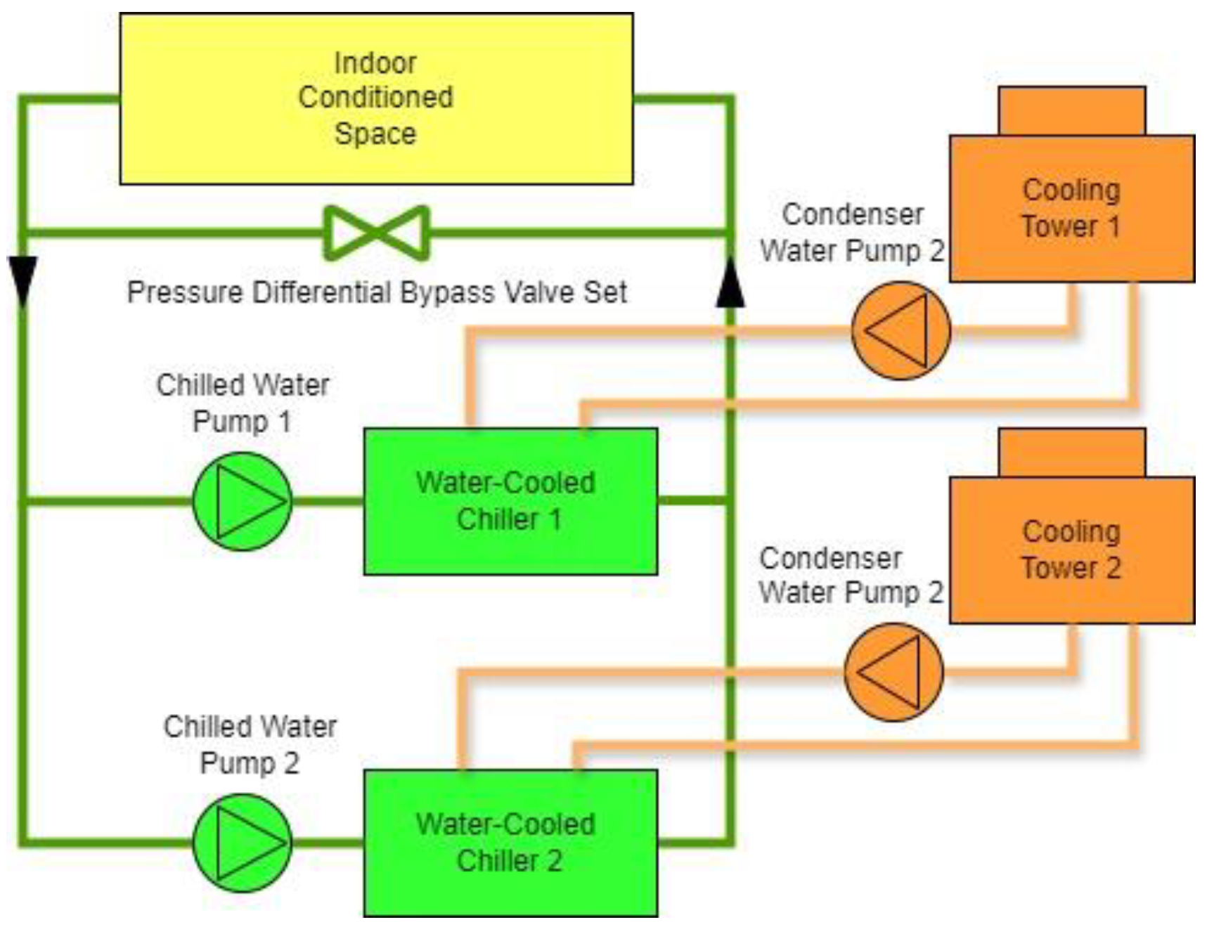
2.1. Relevant Models for CAC Systems

(1)

Mathematical Model of the CH

First, a model of the screw-type water chiller is established. This model can be built based on the model provided by J.M. Gorden [25], and such a model is widely used in the performance analysis and optimization of centrifugal and screw-type water chillers. This model performs well in the medium to high load range (30–100% of the rated load). This model is mainly based on the following two parameters: the outlet water temperature of the CT, t_c,out, and the outlet water temperature of the CH, t_e,out. Among them, when t_c,out increases, the condensing pressure will also increase, and the compressor needs to perform more work to achieve the same cooling effect, thus resulting in a decrease in the COP. Conversely, when the t_c,out decreases, the condensing pressure and the power consumption of the compressor are reduced, leading to an increase in the COP, and, under a certain load, this results in lower energy consumption of the CH.

The mathematical model of the CH is as follows:

$${\displaystyle \frac{1}{\mathrm{COP}}}={\displaystyle \frac{t_{\mathrm{c},\mathrm{out}}}{t_{\mathrm{e},\mathrm{out}}}}-1+{\displaystyle \frac{t_{\mathrm{c},\mathrm{out}}}{t_{\mathrm{e},\mathrm{out}}}}\left[{\displaystyle \frac{1}{Q_e}}+{\displaystyle \frac{1}{C_c{T}_{\mathrm{e},\mathrm{w},\mathrm{out}}}}+{\displaystyle \frac{1}{t_{\mathrm{e},\mathrm{out}}}}({\displaystyle \frac{1}{C_c}}+{\displaystyle \frac{1}{C_e}})\right]q_e+\left[{\displaystyle \frac{1}{C_e{t}_{\mathrm{e},\mathrm{out}}}}+{\displaystyle \frac{1}{t_{\mathrm{e},\mathrm{out}}}}({\displaystyle \frac{1}{C_c}}+{\displaystyle \frac{1}{C_e}})-{\displaystyle \frac{1}{Q_e}}\right]q_c$$

(1)

where COP is the coefficient of performance of the CH; Q_e is the cooling capacity of the CH, kW; Q_c is the heat rejection capacity on the condenser side, kW; t_e,out is the outlet temperature of the chilled water from the chiller in K; q_c is the irreversible loss on the condenser side, q_c = a₄ + a₅R_q + a₆R_q² + a₇R_q³, where a₄, a₅, a₆, and a₇ are coefficients, and R_q is the load ratio; q_e is the irreversible loss on the evaporator side, q_e = a₀ + a₁R_q + a₂R_q² + a₃R_q³, where a₀, a₁, a₂, and a₃ are coefficients; C_c is the heat transfer coefficient of the condenser, kJ/K; and Ce is the heat transfer coefficient of the evaporator, kJ/K.

The power of the CH is calculated as follows:

$$P_{chiller}={\displaystyle \frac{Q_e}{COP}}$$

(2)

where P_chiller is the power of the CH, kW.

(2)

Mathematical Model of Cooling Towers

In the research on cooling tower models, Merkel [26] proposed the mechanism of heat and mass transfer inside the cooling tower, laying a theoretical foundation for subsequent research. Parker and Treybal [27] put forward the first set of design methods for counterflow cooling towers. Currently, when it comes to the energy savings and optimized operation of AC systems, the CT model proposed by Braun is widely recognized [28]. However, the expression of this model is very complex, which is not conducive to solving optimization problems. Therefore, based on this model, this paper fits a large number of data samples. Under the condition of a constant cooling water flow rate, the relationship between the fan frequency and the t_c,out is obtained through fitting. The fitted expression is as follows:

$$\Delta t_{c,out}={\mathrm{c}}_1{\left({\displaystyle \frac{f}{f_0}}\right)}^3+{\mathrm{c}}_2{\left({\displaystyle \frac{f}{f_0}}\right)}^2+c_3\left({\displaystyle \frac{f}{f_0}}\right)+c_4$$

(3)

$$t_{c,out}=\Delta t_{c,out}+t_{a,wb}$$

(4)

$$P_{ct}={\left({\displaystyle \frac{f}{f_0}}\right)}^3{P}_{0,ct}$$

(5)

where Δt_c,out is the difference between the outlet water temperature of the CT and the outdoor wet-bulb temperature; t_a,wb is the outdoor wet-bulb temperature; f is the operating frequency of the CT fan, the range of f is 20~50 Hz; f₀ is the rated frequency of the CT fan, under normal circumstances, the value of this frequency is 50 Hz; c₁, c₂, c₃, c₄ are fitting coefficients, c₁ = −8.3863, c₂ = 27.3613, c₃ = −30.0049, and c₄ = 12.8056; P_ct is the actual operating power of the CT; and P₀,_ct is the rated power of the CT.

(3)

AC Room Model

In the simulation of the AC system, compared with the electromechanical system, the building rooms are characterized by large thermal inertia and a slow thermal response. Moreover, the thermal characteristics of the building can be affected by factors such as thermal disturbances. These characteristics need to be reflected in the room model so that the room temperature calculated can be closer to the actual operating conditions.

In the room model of this paper, the building thermal characteristic coefficients based on the DeST simulation [29] reflect the response characteristics of the building under the actions of thermal disturbances. These thermal disturbances include factors such as outdoor ventilation, solar radiation, long-wave mutual radiation among the inner surfaces of each building envelope, convective heat transfer happening between the exterior surface of the building envelope and outdoor air, radiative heat transfer happening between the exterior surface of the building envelope and the surrounding environment, heat dissipation from indoor occupants and equipment, and the mutual influences among various rooms of the building through heat conduction and ventilation. The basic room temperature represents the indoor air temperature when the building has no cooling or heating system and is affected by various heat generation indoors and outdoors.

In the room thermal model, which is based on the building’s thermal characteristic coefficients and baseline room temperature, the thermal mass effect of the building envelopes is considered. When variations in the AC cooling capacity affect the current room temperature, the model simultaneously accounts for the influence of the current temperature on the subsequent time step’s thermal conditions. Then, the room thermal process under the control of the AC terminal is solved.

Based on the state–space method [30], the DeST software (Version: 20230713) can calculate the thermal characteristic coefficients and the basic room temperature. Using the thermal characteristic coefficients of the room and the amount of thermal disturbances, the hourly temperature of the AC room can be obtained. The calculation time step used is a short time step of 15 min, which is in line with the actual terminal adjustment process.

Calculate the room temperature t_a at the current moment through the thermal characteristic coefficients, the basic room temperature of the room, and the cooling and heating capacity input by the AC terminal. Solve for the cooling and heating capacity q_s that the AC terminal inputs into the room based on the air supply volume of the coil and the supply air temperature.

$$t_{\mathrm{a}}=t_{\mathrm{bz}}+{\phi }_{\mathrm{hvac}}{q}_{\mathrm{s}}$$

(6)

$$q_{\mathrm{s}}=\mathrm{c}\rho G_{\mathrm{s}}(t_{\mathrm{s}}-t_{\mathrm{a}})$$

(7)

By combining Equations (6) and (7), the room temperature at each moment can be determined according to the thermal characteristics of the building and the AC parameters.

$$t_{\mathrm{a}}={\displaystyle \frac{t_{\mathrm{bz}}+{\phi }_{\mathrm{hvac}}{C}_{\mathrm{P}}\rho G_{\mathrm{s}}{t}_{\mathrm{s}}}{1+{\phi }_{\mathrm{hvac}}{C}_{\mathrm{P}}\rho G_{\mathrm{s}}}}$$

(8)

where t_a is the room temperature, °C; t_bz is the room air temperature, which, at the current moment without considering the influence of the AC system, is determined by outdoor meteorological parameters and indoor thermal disturbances and is expressed in °C; φ_hvac is the thermal characteristic coefficient of the room, reflecting the response characteristics generated by some passive thermal disturbances acting on the building; q_s is the cooling and heating energy inputs into the room by the AC system, W; C_p is the air-specific heat capacity, J/kg·°C; ρ is the density of air, kg/m³; G_s is the air supply volume of the air conditioner, m³/s; and t_s is the air supply temperature of the AC system, °C.

(4)

The Cooling Coil Heat Exchange Model

The cooling coil model is established based on the heat and moisture exchange process between the air and the heat exchanger surface [31]. In CAC systems, the temperature and water vapor partial pressure gradients between the bulk air and the boundary layer air adjacent to the heat exchanger surface drive simultaneous heat and mass transfer. Since the chiller’s outlet water temperature is typically maintained at 7 °C, the boundary layer air temperature often falls below the dew point of the bulk air, leading to condensation and dehumidification during the cooling process. The air and the heat exchanger surface simultaneously conduct sensible heat and latent heat exchanges, which complicate the heat exchange calculation under wet working conditions. The degree of heat and moisture exchange of the inlet and outlet fluids of the surface heat exchanger can be characterized by the total heat exchange efficiency E_g. The treatment proportion of the air passing through the surface heat exchanger can be characterized by the general heat exchange efficiency E′. For a specific cooling coil, when the heat exchange between the air and water reaches equilibrium, the following conditions need to be met:

①

The total heat exchange efficiency E_g required in the air treatment process should be equal to the total heat exchange efficiency E_g that the cooling coil can achieve;

②

The general heat exchange efficiency E′ required in the air treatment process should be equal to the general heat exchange efficiency E′ that the cooling coil can achieve;

③

The heat released on the air side should be equal to the heat absorbed on the chilled water side.

Based on these conditions, a mathematical model of cooling coil heat exchange is constructed in this paper.

$$E_g={\displaystyle \frac{1 - \exp [-\beta (1 - \gamma \left)\right]}{1 - \gamma \exp [-\beta (1 - \gamma \left)\right]}}={\displaystyle \frac{t_1-t_2}{t_1 - t_{e,out}}}$$

(9)

$$E^{\prime }=1 - \exp \left({\displaystyle \frac{{\alpha }_w\cdot a\cdot N}{V_y\cdot \rho \cdot C_P}}\right)=1 - {\displaystyle \frac{t_2 - {\mathrm{t}}_{\mathrm{s}2}}{t_1 - {\mathrm{t}}_{\mathrm{s}1}}}$$

(10)

$$G_s\left(h_1 - {\mathrm{h}}_2\right)=\mathrm{m}\mathrm{C}\left(t_{e,out} - t_{e,in}\right)$$

(11)

where E_g is the total heat exchange efficiency; β and γ are coefficients; t₁ is the dry-bulb temperature of the air at the inlet of the coil, °C; t₂ is the dry-bulb temperature of the air at the outlet of the coil, °C; t_e,out and t_e,in are the outlet and inlet water temperatures of the CH in °C; E’ is the general heat exchange efficiency; α_w is the heat transfer coefficient of the outer surface of the coil in kW/(m²·°C); a is the fin-pass coefficient; N is the number of rows of the coil; V_y is the face velocity of the coil, m/s; ρ is the air density, kg/m³; C_p is the specific heat capacity of the air, kJ/(kg·°C); t_s1 and t_s2 are the wet-bulb temperatures of the air at the inlet and outlet of the coil in °C; h₁ is the enthalpy value of the air at the inlet of the coil, kJ/kg; h₂ is the enthalpy value of the air at the outlet of the coil, kJ/kg; m is the flow rate of the chilled water in the coil, kg/s; and C is the specific heat capacity of the chilled water, kJ/(kg·°C).

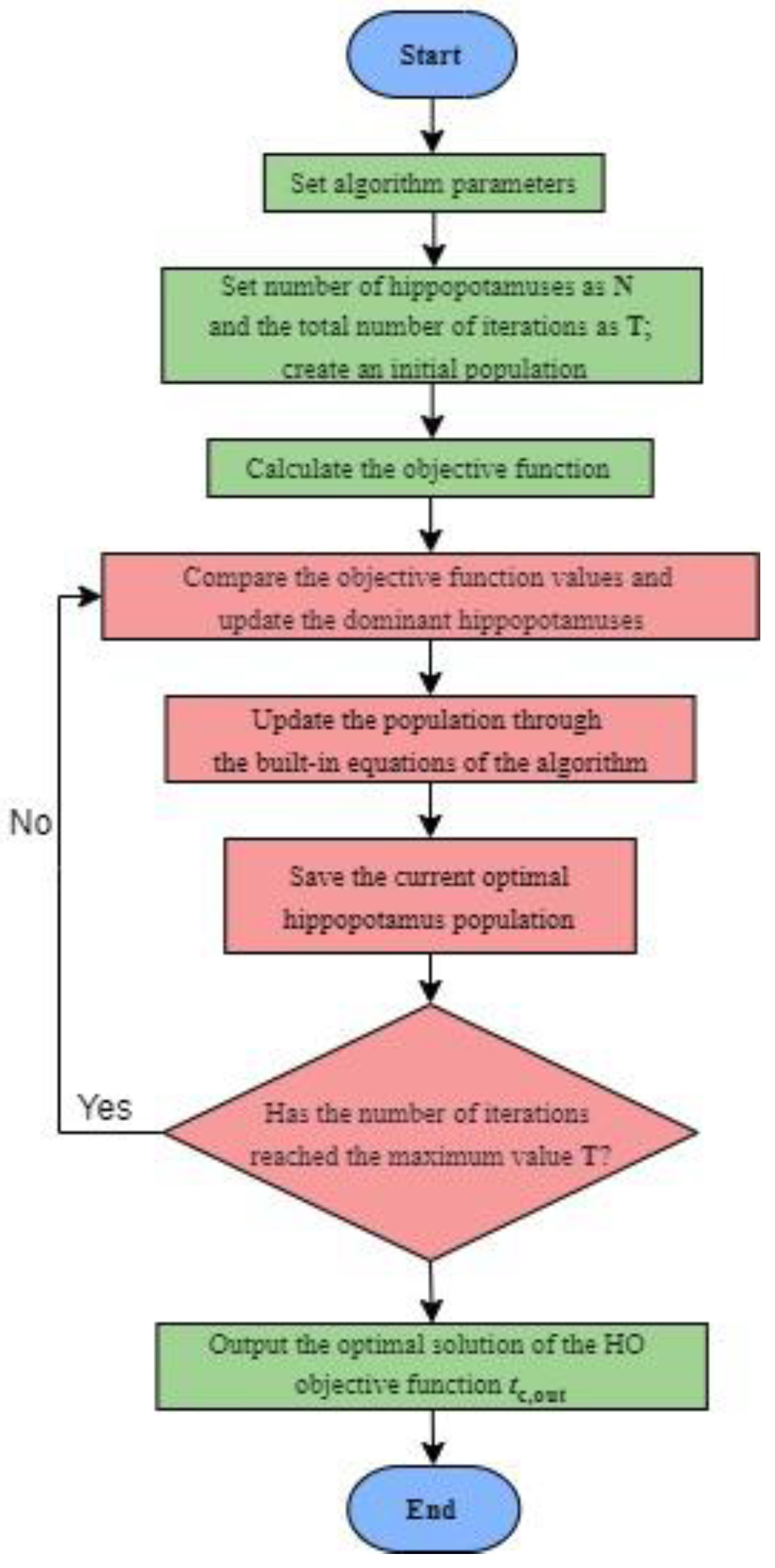
2.2. Solution Optimization with the Hippopotamus Optimization Algorithm (HOA)

The Hippopotamus Optimization Algorithm (HOA) [32] is a population-based intelligent optimization algorithm. It simulates ① the position update of hippos in rivers or ponds, ② the defense strategies against predators, and ③ the methods of escaping from predators, and adaptively adjusts the resolution of the search space and the search speed to quickly and accurately find the optimal solution. It has the characteristics of fast convergence speed and high solution accuracy.

Similar to traditional optimization algorithms, the initialization stage of the HOA involves the generation of random initial solutions. In this step, the following formula is used to generate the vector of decision variables:

$${\chi }_i:x_{i,j}=l{b}_j+r\cdot (u{b}_j-l{b}_j);i=\mathrm{1,2},3\dots ,N_{hippo};j=\mathrm{1,2},3,\dots ,m$$

(12)

where χ_i represents the position of the i-th candidate solution, r is a random number within the range from 0 to 1; lb_j and ub_j, respectively, represent the lower limit and the upper limit of the j-th decision variable; N_hippo represents the population size of hippos in the herd; and j represents the number of decision variables in the problem. The population matrix is represented by Equation (13)

$$\chi ={\left[\begin{array}{c}{x}_1\\ ⋮\\ x_i\\ \begin{array}{c}⋮\\ x_N\end{array}\end{array}\right]}_{N\times m}=\left[\begin{array}{ccccc}{x}_{\mathrm{1,1}}& \dots & x_{1,j}& \dots & x_{1,m}\\ ⋮& \ddots & ⋮& ⋰& ⋮\\ x_{i,1}& \dots & x_{i,j}& \dots & x_{i,m}\\ ⋮& ⋰& ⋮& \ddots & ⋮\\ x_{N,1}& \dots & x_{N,j}& \dots & x_{N,m}\end{array}\right]$$

(13)

In the equation, each vector χi represents the i-th “hippo”, that is, the solution to the problem. After each iteration of the HOA is completed, these “hippos” (i.e., all population members) will be updated according to the first to third stages through the formulas built into the algorithm, and then the “dominant hippos”, which are the optimal solutions under the current number of iterations, will be screened out. The process of updating the population based on the equations continues until the final iteration. During the execution of the algorithm, the best potential solution is consistently tracked and stored. After the entire algorithm is completed, the best candidate solution, that is, the dominant hippo solution, is announced as the final solution to the problem. In the process of the MATLAB co-simulation model, within each time step, the HOA is used to search for the t_c,out under the optimal operating points in order to achieve control of the air-conditioning system in the shortest possible time. Figure 1 shows the flow chart of the HOA search and optimization process.

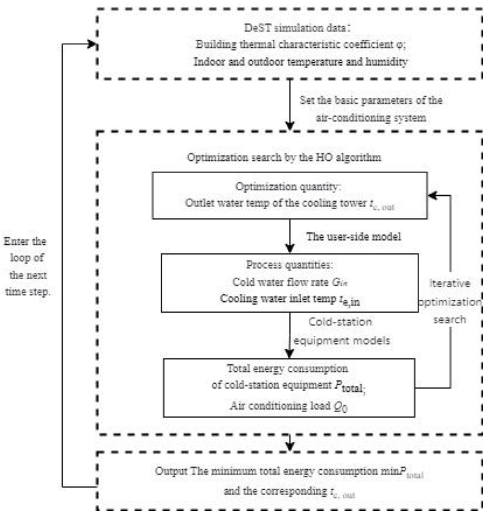
2.3. Simulation Calculation Process

In this paper, based on the overall user-side model with a continuously adjustable terminal and the cold-station model, the HOA is used to search for the operating conditions that reduce the power consumption of the CH and the CT to the minimum. Using t_c,out as the optimization variable, a dynamic co-simulation of the user side and cooling station is performed, with the objective of minimizing the energy consumption of both the CH and CT. Through this optimization, the optimal control setpoint for t_c,out is determined. The calculation process is shown in Figure 2.

First, the DeST software is used to model the building, and the basic parameters of the AC rooms are set, including elements such as room usage, occupancy rate, AC start–stop times, and thermal disturbances from equipment and lighting. After completing the settings, the building thermal characteristic coefficients associated with the AC cooling capacity can be generated. These parameters, together with basic parameters such as humidity and outdoor temperature, are extracted and used for simulation calculations.

Each building room is equipped with continuously adjustable AC terminals. All the rooms and their AC terminals together form the user side. The main equipment of the cold station includes the CH, CT, and chilled and cooling water circulation pumps (the modeling of the water network is ignored in this paper), which as a whole form the cold-station side.

The total chilled flow rate G_w and the chilled return temperature t_e,in of the system are calculated by the user-side model and input to the cold-station equipment model. The power P of each equipment and the total power P_total and the air-conditioning load Q₀ under the current working condition are calculated by the cold-station equipment model. Then, the optimization search is performed using the HOA. If the optimization result is the optimal value, the optimal working condition point, the optimal power, and the parameters of each equipment under the optimal working conditions are output, and the calculation of the next time step is entered. If not, the working condition point is updated and a new round of iterative calculation is carried out. Eventually, the minimum total energy consumption of typical daily equipment including cooling towers and chillers is obtained.

3. Case Study

3.1. Room Parameter Settings

The commercial building in Beijing is selected as the simulated building (Figure 3). The building has a floor area of 9604 m², and the AC room area is 9280 m². The building has a total of four floors with a floor height of 4.2 m. There are four open-plan commercial zones on each floor, and there is a corridor and elevator shaft in the middle of the building. The standard floor plan layout is shown in Figure 4.

Table 1. Basic information settings of the building.

Category	Parameter
City	Beijing
Building Use	Commercial building
Air-Conditioning zone	9280 m²
Number of Floors	4
Exterior Wall Thermal Parameters	Exterior wall heat transfer coefficient K = 0.265 W/(m²·K)
Exterior Window Thermal Parameters	Exterior window heat transfer coefficient K = 1.000 W/(m²·K), solar heat gain coefficient (SHGC) = 0.426
Window-to-Wall Ratio	S = 0.35, E/W = 0.3, N = 0.25

shows the basic information of the building.

3.2. Simulation Setup of the AC System

Each room is equipped with several continuously adjustable AC terminals. The water system is a primary pump variable-flow system, and its structure is shown in Figure 5. The designed total chilled water flow rate of the system is 29.76 L/s. The chiller and the chilled water pump adopt a one-to-one matching mode. Based on the building load, two CHs with a rated cooling capacity of 350 kW are selected. The upper limit of the frequency of the chilled water pump is 50 Hz, and the lower limit is 20 Hz, with a rated power of 18 kW. The cooling water pump has a rated power of 20 kW and operates at a fixed frequency. The cooling tower is a counter-flow cooling tower, with one chiller corresponding to one tower, and its rated frequency is f₀ Hz (f₀ = 50).

Table 2. Equipment configuration of the cold station in commercial buildings.

Equipment Name	Specification	Rated Power/kW	Quantity/Unit	Remarks
Chiller	30HXY080A, Chilled water: 7 °C/12 °C, Cooling water: 30 °C/35 °C	350	2	Screw-type variable-frequency unit
Chilled Water Pump	17 L/s, 25 mH₂O	18	2	Variable-frequency pump
Cooling Water Pump	20 L/s, 20 mH₂O	20	2	Fixed-frequency pump
Cooling Tower	HMK-150-10	5	2	Variable-frequency fan

shows the specific parameters of the equipment.

The AC operation period is designed to be from 7:00 to 21:00. The room temperature is set at 26 °C and maintained within the range of 25 °C to 27 °C.

3.3. Design of the Simulation Scheme

To compare the operating energy consumption of various operation modes, three operation strategies are designed:

Strategy 1—The CT operates at the rated power frequency, and the t_c,out is not controlled.

Strategy 2—The t_c,out is set at fixed values of 30 °C, 31 °C, 32 °C, and 33 °C. The frequency of the CT fan is controlled to adjust its air volume so that the t_c,out is controlled to the set point.

Strategy 3—The t_c,out is obtained through optimization. The frequency of the CT fan is controlled to adjust its air volume so that the water temperature leaving the CT is controlled to the set point.

A time step of 15 min is selected, and an optimization calculation is carried out for the control set point. The HOA is used, and the objective function is to minimize the overall operating power of the CH and the CT. The objective function is as follows:

$$\min P_{total}={\displaystyle \sum _{i=1}^{N_{chiller}}{P}_{chiller}}+{\displaystyle \sum _{i=1}^{N_{ct}}{P}_{coolingtower}}$$

(14)

where P_total is the total power, kW; P_chiller is the power of a single CH, kW; P_{cooolingtower} is the power of a single CT, kW; N_chiller is the number of CHs; and N_ct is the number of CTs.

4. Results and Discussion

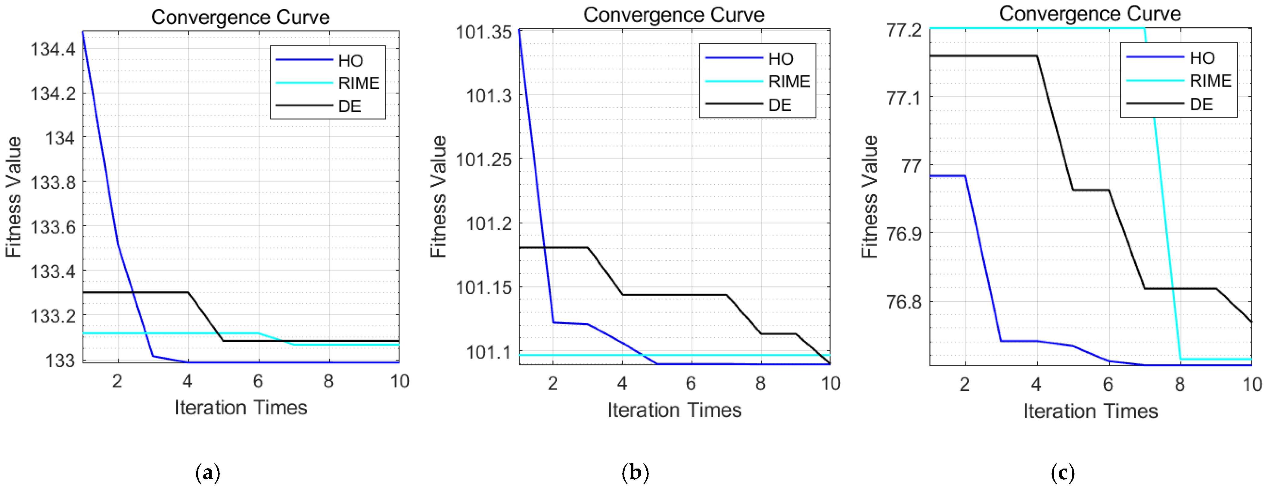
4.1. Algorithm Validation

To verify the superiority of the HOA in optimizing the outlet water temperature of the CT, another new optimization algorithm, the Rime Optimization Algorithm (RIME) [33], and a traditional algorithm, the Differential Evolution Algorithm (DE) [34], were selected for comparison with the HOA under different load rates. To guarantee the calculation velocity, the iteration count was set at 10.

Three operating conditions with chiller load rates of 50%, 70%, and 90% were selected to optimize the optimal operating conditions of the t_c,out, and the optimal fitness values were calculated. The minimum operating powers of the CH and the CT under different CH load rates for the three algorithms are shown in

Table 3. Optimization results for the operating power using different algorithms.

Chiller Load Rate	Minimum Operating Power kW
	HO	RIME	DE
90%	132.9871	133.0667	133.0833
70%	101.0893	101.0966	101.0897
50%	76.7057	76.7146	76.7686

. The change curves of the fitness values of each algorithm under the three operating conditions are shown in Figure 6.

All three algorithms can find relatively good fitness values. However, the HOA performs more outstandingly during the optimization process, and the optimized fitness value is the smallest. As can be seen in Figure 6, when calculating the optimal operating point within one time step, the function converges when the number of iterations is five. It only takes 1.96 s to complete the optimization of one time point when running in MATLAB, which shows a relatively fast optimization speed. This makes it suitable for fast and dynamic optimization solutions in air-conditioning systems. Therefore, this algorithm is adopted for optimization in Strategy 3.

4.2. Operating Results of the Strategies

Figure 7 shows the changes in AC electrical load and the temperature of the AC room within 24 h under Strategy 1. At night, when the AC is off, the accumulation of indoor residual heat causes the indoor temperature to rise continuously. The AC electrical load is relatively large at 7:00 when the AC system is turned on. Subsequently, as the indoor temperature decreases, the AC electrical load tends to stabilize. From 14:00–16:00 in the afternoon, the indoor temperature rises slightly, but still remains within the temperature control range. Then, as time goes by, the AC electrical load gradually decreases.

Figure 8, Figure 9 and Figure 10, respectively, present the calculated operating power results for the CH and the CT under the three strategies at three different times. For each case, the leftmost data point represents the system’s operating results under Strategy 1. The optimized operating condition corresponds to the results under Strategy 3, and the operating conditions with outlet water temperatures of 30 °C, 31 °C, 32 °C, and 33 °C are the operating results of the system under Strategy 2.

Figure 8 shows the results at 9:00. It indicates that at this moment, the wet-bulb temperature is 28.3 °C. Under Strategy 1 where the t_c,out is not controlled, the inlet water temperature of the CT is 34.7 °C, the outlet water temperature is 29.8 °C, the power of the CT operating at the rated frequency is 10.00 kW, the corresponding power consumption of the chillers is 118.0 kW, and the total power of the CH and the CT is 128.0 kW. Under Strategy 2, when the set value of the t_c,out varies from 30 °C to 33 °C, the power consumption of the CT fans shows a monotonically decreasing trend. This indicates that as the set temperature rises, the CT fan power consumption it controls continuously decreases. Due to the increase in the outlet water temperature of the CT, the energy consumption of the CH rises. This is consistent with the variation law of the energy consumption of the CH and the CT in Reference [35]. That is, with the change in the t_c,out, the operating powers of the CH and the CT show a “compensatory” variation law. Meanwhile, when the t_c,out increases by 1 °C under the operating conditions of 30 °C, 31 °C, 32 °C, and 33 °C, the operating power of the CH increases by 3.71%, 3.53%, and 3.51%, respectively. This is completely in line with the operating law described in Reference [36], proving the reliability of the simulation results. Under Strategy 3, the optimized outlet temperature of the CT set value is 30.6 °C. The power of the CT is 4.0 kW, the power consumption of the CH is 121.5 kW, and the total power of the CH and the CT is 125.5 kW. By comparing the results of different strategies, it is found that the power consumption of the CH and the CT corresponding to the optimized outlet temperature of the CT set value under Strategy 3 is the lowest.

Table 4. Comparison of cooling tower operating conditions under different strategies at 9:00.

	Set Temperature (°C)	Fan Frequency (HZ)	tc,out (°C)
Strategy 1	-	50	29.8
Strategy 2	30	47	30
	31	32	31
	32	25	32
	33	20	33
Strategy 3	Obtained by optimization	37	30.6

presents the results of the power, frequency of the CT fan, and the water temperature difference under different strategies. The results show that as the set value of the t_c,out increases, the frequency of the CT fan decreases, the air volume of the fan is reduced, and the power decreases. Under Strategy 1, since the t_c,out is not controlled, the fan operates at the rated frequency f₀. The power output of the CT fan is the largest, the t_c,out is the lowest, and the power of the chiller is the lowest. Under Strategy 3, the fan frequency and power are relatively low, and the t_c,out is higher than that of Strategy 1. This indicates that under the uncontrolled condition of Strategy 1, although the t_c,out is low, the fan pays a high price for it. Meanwhile, under Strategy 3, the optimized outlet water temperature takes into account the corresponding energy consumption of the CH, and the power output of the fan is precisely optimized, minimizing the energy consumption of both the CH and the CT.

Figure 8 and Figure 9, respectively, present the results of equipment power consumption varying with the t_c,out at 9:00 and 14:00. Both figures reflect the same pattern: as the t_c,out at that moment rises, the power of the CT gradually decreases while the power of the CH gradually increases, reaching the minimum value under the optimal operating condition.

The main difference between the two is that when the t_c,out operates according to the designed operating condition, it sometimes fails to reach the temperature control point. As shown in Figure 9, when the t_c,out is controlled at 30 °C, the actual t_c,out is 30.6 °C. At this time, the temperature set point is too close to the wet-bulb temperature. Even though the CT fan reaches its maximum power output, it cannot control the temperature at this point, and the actual control effect is equivalent to that of Strategy 1.

Figure 10 also reflects the problem that the t_c,out under Strategy 2 cannot reach the set point. The two control points of 30 °C and 31 °C completely fail, and the t_c,out is the same as that in the uncontrolled case. By comparing Figure 8, Figure 9 and Figure 10, it is found that the optimal operating conditions occur in different temperature setting intervals at different times. The HOA algorithm can accurately determine the position of the optimal operating point.

By comparing the three different times of 9:00, 14:00, and 15:00, this paper analyzes the impacts of the change in the t_c,out control set value from 30 °C to 33 °C on the power of the CH and the CT. At a certain moment of a typical day, with the t_a,wb remaining unchanged, as the control set value increases, the power of the CH gradually increases, while the power of the CT shows a decreasing trend. Compared with the CH, the power consumption of the CT accounts for a relatively small proportion, but the change in its t_c,out has a significant impact on the power consumption of the CH.

As can be seen in Figure 8, Figure 9 and Figure 10, due to the varying AC loads at different times, the optimal operating points occur among different temperature set values. The energy consumption of the AC operating under the optimal condition is consistently lower than that under other conditions. This proves that this method is accurate and feasible in optimizing the operating conditions of the t_c,out.

After calculating and solving the optimal operating conditions for each moment of the whole day, the optimal t_c,out and relevant curves are obtained, as shown in Figure 11. The data in the figure indicates that the optimal t_c,out is not a fixed value during a certain period. Instead, it is a curve that has a similar changing trend to the t_a,wb. The Δt_c,out is between 2 °C and 3 °C, and it has nothing to do with the outdoor dry-bulb temperature of the day. At 3:00, the wet-bulb temperature of the outdoor air reaches its highest value, and the outlet water temperature of the cooling tower also peaks. At this moment, t_c,out = 32.2 °C. It can be seen that the optimized t_c,out has a strong correlation with the wet-bulb temperature of the day. The temperature difference between the inlet and outlet of the cooling water also varies throughout the day. At 7:00, t_c,out = 35.9 °C and t_c,out = 30.7 °C. At this time, the temperature difference is largest. At 21:00, t_c,out = 32.7 °C and t_c,out = 30.8 °C, At this moment, the temperature difference is the smallest. This is caused by the fact that the loads at different moments of the day are different, and when the flow rate of the cooling water remains unchanged, the amount of condensing heat carried away is different.

Figure 12 shows the changes in the total energy consumption of the CH and the CT during the AC operating period under Strategy 1 and Strategy 3. Compared with Strategy 1, Strategy 3 has a good energy-saving effect during the AC operation period, with a maximum energy-saving rate of 4.5%. The total energy-saving rate within a typical day is 3.2%.

It can be seen in Figure 12 that the energy-saving rate at the moment when the Ac is started is the lowest at only 1.85%. At this time, the AC load is relatively large, the energy consumption of the CH is high, and the influence of the t_c,out on the chiller is relatively small.

As time goes by, the changing trend of the energy-saving rate is completely opposite to the variation law of the wet-bulb temperature of the day. It reaches a trough value at 15:00, and the energy-saving rate is 2.4%. At this time, the t_a,wb is the highest, and there is relatively little space for optimizing the t_c,out.

Moreover, the energy-saving rate is the highest at 9:00. At this time, the wet-bulb temperature is the lowest, there is a large space for optimization, the load throughout the day is the lowest, and the energy consumption of the cooling tower accounts for a relatively high proportion of the total energy consumption of the system.

In practical applications, both Strategy 1 and Strategy 2 have their respective suitable scenarios. In Strategy 1, the CT fan operates at a constant rated frequency, featuring simple control, high reliability, and no need for complex feedback control systems, resulting in lower investment costs. However, its energy consumption is high, especially in part-load conditions, leading to significant energy waste. Strategy 2 operates at fixed set points and can stabilize the t_c,out at the preset values through feedback control, which is easy to implement in engineering. Nevertheless, it also lacks flexibility and relies on manual experience for setting values. As a new-type control strategy, Strategy 3 offers advantages such as global efficiency optimization, strong dynamic adaptability, and low long-term operating costs, making it more suitable for large-scale complex systems and high-energy-consumption scenarios. Despite its high system complexity, with the development of technology, it is bound to achieve broader applications.

5. Conclusions

In this paper, a joint simulation model of the user side and the cold station based on MATLAB was established. Considering the coupling between the AC terminal and the room, the variation in the energy consumption of the AC cold-station equipment over time was analyzed. The HOA was used to search for the optimal operating point of the CAC system. The t_c,out was selected as the main variable affecting the AC energy consumption. The optimal operating set values of the equipment under the load and environmental conditions within a typical day for the CAC system were solved. Finally, an optimized operation control strategy was developed for the CAC system. By analyzing the energy consumption variations of both the CH and CT before and after optimization, the energy-saving potential of the optimized operating condition was quantified, and the overall system performance under optimal control was validated. The specific conclusions are as follows:

(1)

A joint simulation model of the user side and the cold station based on MATLAB was constructed. This model adopts a calculation method with a small time step (15 min), which can reflect the dynamic operation process of the AC at each moment. Taking into account the coupling between the air-conditioning terminal and the room, it can analyze the room temperature and the energy consumption.

(2)

A new population-based algorithm, HOA, was employed. Under three operating conditions of the chiller load rate, namely, 50%, 70%, and 90%, the optimal operating condition of the t_c,out was searched. By comparing the HOA with two other algorithms, it was found that all three algorithms could find relatively good fitness values. However, the HOA demonstrated more excellent performance during the optimization process, with the smallest fitness value after optimization. The function converges when the number of iterations is five, and it only takes 1.96 s to complete the optimization for one moment when running in MATLAB.

(3)

By controlling the t_c,out to keep it in the optimal operating condition, the system achieves a maximum daily energy-saving rate of 4.5% and a total energy-saving rate of 3.2% compared to conventional non-optimized operation.

6. Limitations and Future Scope

Overall, this study presents an optimization strategy for operating condition points in the coupled operation of building and AC systems. This strategy holds certain value for the simulation of building and AC systems and their energy-saving applications in practical engineering. During the optimization process, this paper utilizes a novel optimization algorithm, the Hippopotamus Optimization Algorithm, to search for the optimal operating condition points of the outlet water temperature of the CT, aiming to reduce AC system energy consumption. Based on the algorithm optimization, future research will focus on the integration of buildings with photovoltaic and energy storage systems. The operation of system equipment will no longer be restricted by energy availability. Instead, the algorithm will aim to optimize relevant operating conditions with the goals of indoor thermal comfort and the utilization rate of renewable energy, which is “contrary” to the current goal of minimizing energy consumption. In terms of the model, this paper is limited to the research of methods. An equal-scale model identical to the real building has not been established, and the construction of a detailed water network model has been overlooked. In subsequent research, efforts should be made to improve the accuracy of the model to make it more applicable to practical engineering.

References

1. Kim, J.H.; Seong, N.C.; Choi, W. Forecasting the energy consumption of an actual air handling unit and absorption chiller using ANN models. Energies 2020, 13, 4361. [Google Scholar] [CrossRef]
2. Ma, H.T.; Du, N.; Yu, S.J.; Lu, W.Q.; Zhang, Z.Y.; Deng, N.; Li, C. Analysis of typical public building energy consumption in northern China. Energy Build. 2017, 136, 139–150. [Google Scholar] [CrossRef]
3. Wang, N.; Phelan, P.E.; Harris, C.; Langevin, J.; Nelson, B.; Sawyer, K. Past visions, current trends, and future context: A review of building energy, carbon, and sustainability. Renew. Sustain. Energy Rev. 2018, 82, 976–993. [Google Scholar] [CrossRef]
4. Zaki, A.M.; Zayed, M.E.; Alhems, L.M. Leveraging machine learning techniques and in-situ measurements for precisely predicting the energy performance of regenerative counter-flow indirect evaporative cooler in a semi-arid climate building. J. Build. Eng. 2024, 95, 110318. [Google Scholar] [CrossRef]
5. Xu, Y.; Gao, W.J.; Qian, F.Y.; Li, Y.X. Potential analysis of the attention-based LSTM model in ultra-short-term forecasting of building HVAC energy consumption. Front. Energy Res. 2021, 9, 730640. [Google Scholar] [CrossRef]
6. Seong, N.C.; Kim, J.H.; Choi, W. Optimal control strategy for variable air volume air-conditioning systems using genetic algorithms. Sustainability 2019, 11, 5122. [Google Scholar] [CrossRef]
7. Xie, K.; Hui, H.; Ding, Y.; Song, Y.; Ye, C.; Zheng, W.; Ye, S. Modeling and control of central air conditionings for providing regulation services for power systems. Appl. Energy 2022, 315, 119035. [Google Scholar] [CrossRef]
8. Jiang, H.; Qiu, S.; Ran, B.; Song, S.; Long, J. Energy-saving regulation methods and energy consumption characteristics of office air-conditioning loads in hot summer and cold winter areas. Energy Built Environ. 2024, in press. [Google Scholar] [CrossRef]
9. Zheng, Z.X.; Li, J.Q.; Duan, P.Y. Optimal chiller loading by improved artificial fish swarm algorithm for energy saving. Math. Comput. Simul. 2019, 155, 227–243. [Google Scholar] [CrossRef]
10. Zaki, A.M.; Zayed, M.E.; Bargal, M.H.S.; Saif, A.G.H.; Chen, H.; Rehman, S.; Alhems, L.M.; El-deen, E.H.N. Environmental and energy performance analyses of HVAC systems in office buildings using boosted ensembled regression trees: Machine learning strategy for energy saving of air conditioning and lighting facilities. Process Saf. Environ. Prot. 2025, 198, 107214. [Google Scholar] [CrossRef]
11. Ma, Z.J.; Wang, S.W. Supervisory and optimal control of central chiller plants using simplified adaptive models and genetic algorithm. Appl. Energy 2011, 88, 198–211. [Google Scholar] [CrossRef]
12. Zhu, D.D.; Hong, T.Z.; Yan, D.; Wang, C. A detailed loads comparison of three building energy modeling programs: EnergyPlus, DeST and DOE-2.1E. Build. Simul. 2013, 6, 323–335. [Google Scholar] [CrossRef]
13. Coakley, D.; Raftery, P.; Keane, M. A review of methods to match building energy simulation models to measured data. Renew. Sustain. Energy Rev. 2014, 37, 123–141. [Google Scholar] [CrossRef]
14. Seo, B.; Yoon, Y.B.; Mun, J.H.; Cho, S. Application of Artificial Neural Network for the Optimum Control of HVAC Systems in Double-Skinned Office Buildings. Energies 2019, 12, 4754. [Google Scholar] [CrossRef]
15. Lee, W.S.; Chen, Y.T.; Wu, T.H. Optimization for ice—Storage air-conditioning system using particle swarm algorithm. Appl. Energy 2009, 86, 1589–1595. [Google Scholar] [CrossRef]
16. Wang, J.J.; An, D.W.; Zhang, C.F.; Jing, Y.Y. Genetic optimization algorithm of PID decoupling control for VAV air-conditioning system. Trans. Tianjin Univ. 2009, 15, 308–314. [Google Scholar] [CrossRef]
17. Yao, Y.; Chen, J. Global optimization of a central air-conditioning system using decomposition–coordination method. Energy Build. 2010, 42, 570–583. [Google Scholar] [CrossRef]
18. Zhou, X.W.; Yu, J.Q.; Zhang, W.H.; Zhao, A.J.; Zhou, M. A multi-objective optimization operation strategy for ice—Storage air-conditioning system based on improved firefly algorithm. Build. Serv. Eng. Res. Technol. 2022, 43, 161–178. [Google Scholar] [CrossRef]
19. García Ruiz, A.H.; Ibarra Martínez, S.; Castán Rocha, J.A.; Terán Villanueva, J.D.; Laria Menchaca, J.; Treviño Berrones, M.G.; Ponce Flores, M.P.; Santiago Pineda, A.A. Assessing a Multi-Objective Genetic Algorithm with a Simulated Environment for Energy-Saving of Air Conditioning Systems with User Preferences. Symmetry 2021, 13, 344. [Google Scholar] [CrossRef]
20. Yang, S.Y.; Yu, J.Q.; Gao, Z.K.; Zhao, A.J. Energy-saving optimization of air-conditioning water system based on data-driven and improved parallel artificial immune system algorithm. Energy Convers. Manag. 2023, 283, 116902. [Google Scholar] [CrossRef]
21. Feng, Z.X.; Wang, W.J.; He, X.; Li, G.T.; Zhang, L.T.; Xiang, W.P. Energy Saving Optimization of Chilled Water System Based on Improved Fruit Fly Optimization Algorithm. ASME J. Therm. Sci. Eng. Appl. 2023, 15, 081010. [Google Scholar] [CrossRef]
22. Zheng, Z.X.; Li, J.Q. Optimal chiller loading by improved invasive weed optimization algorithm for reducing energy consumption. Energy Build. 2018, 161, 80–88. [Google Scholar] [CrossRef]
23. Cen, J.; Zeng, L.Z.; Liu, X.; Wang, F.Y.; Deng, S.J.; Yu, Z.W.; Zhang, G.M.; Wang, W.Y. Research on energy-saving optimization method for central air conditioning system based on multi—Strategy improved sparrow search algorithm. Int. J. Refrig. 2024, 160, 263–274. [Google Scholar] [CrossRef]
24. Gao, Z.K.; Yu, J.Q.; Zhao, A.J.; Hu, Q.; Yang, S.Y. Optimal chiller loading by improved parallel particle swarm optimization algorithm for reducing energy consumption. Int. J. Refrig. 2022, 136, 61–70. [Google Scholar] [CrossRef]
25. Gordon, J.M.; Ng, K.C.; Chua, H.T. Centrifugal chillers: Thermodynamic modelling and a diagnostic case study. Int. J. Refrig. 1995, 18, 253–257. [Google Scholar] [CrossRef]
26. Merkel, F. Verdunstungskühlung V D I. Forschungsarbeiten. In Heat and Mass Transfer Handbook; VDI: Berlin, Germany, 1925; Volume 275, pp. 1–48. [Google Scholar]
27. Parker, R.O.; Treybal, R.E. The heat and mass transfer characteristics of evaporative coolers. In Chemical Engineering Progress Symposium; American Institute of Chemical Engineers: New York, NY, USA, 1961; Volume 57, pp. 138–149. [Google Scholar]
28. Braun, J.E.; Klein, S.A.; Mitchell, J.W. Effictiveness Models for Cooling Towers and Cooling Coils. In Proceedings of the 1989 ASHRAE Annual Meeting, Vancouver, BC, Canada, 25–28 June 1989. [Google Scholar]
29. Xie, X.N.; Song, F.T.; Yan, D.; Jiang, Y. Building Environment Design Simulation Software DeST (2): Dynamic Thermal Process of Buildings. Heat. Vent. Air Cond. 2004, 34, 35–47. [Google Scholar]
30. Jiang, Y. State-Space Method for Analysis of the Thermal Behavior of Room and Calculation of Air Conditioning Load. ASHRAE Trans. 1981, 88, 122–132. [Google Scholar]
31. Yan, D.; Zhang, Y.; Jiang, Y. Building Environment Design Simulation Software DeST (7): Simulation and Analysis of Air Handling Process. Heat. Vent. Air Cond. 2005, 35, 49–58. [Google Scholar]
32. Amiri, M.H.; Hashjin, N.M.; Montazeri, M.; Mirjalili, S.; Khodadadi, N. Hippopotamus Optimization Algorithm: A Novel Nature-Inspired Optimization Algorithm. Sci. Rep. 2024, 14, 5032. [Google Scholar] [CrossRef]
33. Su, H.; Zhao, D.; Heidari, A.A.; Liu, L.; Zhang, X.Q.; Mafarja, M.; Chen, H. RIME: A physics-based optimization. Neurocomputing 2023, 532, 183–214. [Google Scholar] [CrossRef]
34. Storn, R.; Price, K. Differential evolution—A simple and efficient heuristic for global optimization over continuous spaces. J. Glob. Optim. 1997, 11, 341–359. [Google Scholar] [CrossRef]
35. Xie, D.W. Research on Optimization Control of Air Conditioning Cooling Water System. Master’s Thesis, Huazhong University of Science and Technology, Wuhan, China, May 2019. [Google Scholar]
36. Jiang, M.Y. Effect of Operating Conditions on Performance of Chillers. Chin. J. Refrig. Technol. 2021, 41, 78–82. (In Chinese) [Google Scholar]
Figure 1. Flow chart of the HOA.
Energies 18 02476 g001
Figure 2. Operating process of system optimization.
Energies 18 02476 g002
Figure 3. Three-dimensional model of a commercial building.
Energies 18 02476 g003
Figure 4. Floor plan for the standard floor of the commercial building.
Energies 18 02476 g004
Figure 5. System diagram of the cold station and the user side.
Energies 18 02476 g005
Figure 6. Graphs of the changes in the fitness values of each algorithm under different load rates: (a) the changes in the fitness values of each algorithm under a 90% load rate; (b) the changes in the fitness values of each algorithm under a 70% load rate; and (c) the changes in the fitness values of each algorithm under a 50% load rate.
Energies 18 02476 g006
Figure 7. The room temperature and AC electrical load of Strategy 1.
Energies 18 02476 g007
Figure 8. The changes in equipment power consumption with the outlet water temperature of the CT (9:00).
Energies 18 02476 g008
Figure 9. The changes in equipment power consumption with the outlet water temperature of the CT (14:00).
Energies 18 02476 g009
Figure 10. The changes in equipment power consumption with the outlet water temperature of the CT (15:00).
Energies 18 02476 g010
Figure 11. The curves of cooling water and ambient temperature.
Energies 18 02476 g011
Figure 12. Comparison of the energy consumption of different operation strategies.
Energies 18 02476 g012