A Control Framework for the Proton Exchange Membrane Fuel Cell System Integrated the Degradation Information

Abstract

To solve the control problem of the performance degradation of proton exchange membrane fuel cells (PEMFCs), a novel control framework based on the performance degradation is proposed. This control framework introduces the results of the state of health (SoH) estimation and remaining useful lifetime (RUL) prediction, which were used for the controller design because they determine the PEMFC output power. Furthermore, the information of SoH and RUL could be reflected the PEMFC health state and provided maintenance recommendations. The desired power of the stack was obtained, which was used as the real-time desired power of the PEMFC system by synthesizing the RUL, SoH, and ECU information of the stack. The results showed that when the PEMFC system used the designed control framework, the RUL and SoH information could be provided. The stack temperature showed an increasing and then decreasing trend, which indicates that the stack temperature was still controllable by controlling the speeds of the pump and fan.

1. Introduction

Proton exchange membrane fuel cell (PEMFCs) have broad application prospects because they have the advantages of zero emission, high power density, low noise, and short hydrogen filling time. However, the performance degradation seriously restricts their commercial development and increases the difficulty of controlling other auxiliary subsystems, which put forward high requirements for the design of a PEMFC control system. The whole proton exchange membrane fuel cell (PEMFC) system consists of several subsystems such as the stack, air/hydrogen supply, thermal management, and DC/DC subsystems. Among them, the performance degradation of the stack has a significant influence on the whole system compared with other auxiliary subsystems, and the stack durability is the worst. When the PEMFC performance decays, its output performance decreases, with other subsystem conditions unchanged. If the control strategy employed during the initial stage is subsequently utilized for the PEMFC control, this may result in more serious faults during operation and exacerbate the PEMFC performance degradation. Therefore, it is necessary to design a novel PEMFC system controller to control the PEMFC system where the controller synthesizes the operating data information and fuel cell health status to extend its life.

A series of studies on the control issues of PEMFC systems have been conducted. Onanena et al. [1] pointed out that durability is one of the limiting factors for the commercialization of FC technology, and proposed two pattern recognition methods to predict the operation time of the FC by extracting features from electrochemical impedance spectroscopy (EIS) measurements. The first method empirically extracts specific points of the impedance spectrum as features, and the second builds a parametric model by extracting features from the real and imaginary parts of the impedance spectrum, respectively. An experimental dataset was used to assess the effectiveness of the above methods, and the results showed that with an operation time of 1000 h, the average error of the first method was 214 h, while that of the second method was 95 h. Zenith et al. [2] analyzed the controllability of the FC system and designed a control structure for a commercial stationary micro cogeneration system. They contend that the FC is the core component of the system, and is the most critical component in terms of durability. Therefore, the design was focused on optimizing the FC lifetime. They proposed a three-layer control approach based on the original control structure: the first is used for the basic functions of the control system, the second is interfaced with a diagnostic tool to handle reversible degradation phenomena, and the third is interfaced with a prediction tool based on the prognostic and health management (PHM) to set up nominal operating conditions to maximize the FC lifetime. Fletcher et al. [3] argued that the cost and reliability of the FC were the main obstacles preventing FC hybrid vehicles from entering the mainstream market. They pointed out that the operating conditions of the FC can seriously affect its decline, and proposed that the decline can be mitigated by optimizing the energy management strategy (EMS). They designed an optimal EMS for low-speed campus vehicles by using stochastic dynamic programming (SDP) to minimize the fuel consumption and FC degradation. The results showed that the use of SDP could extend the FC life by 14% with a 3.5% increase in fuel consumption because of the avoidance of transient load variations of the stack. Jouin et al. [4] conducted short-term and long-term predictions of PEMFC stacks based on the particle filter (PF) method because of the different time scales of PEMFCs. They determined an adaptive PF configuration to achieve an accurate state of health (SoH) estimation with a high determination coefficient by conducting different data reduction. Fu et al. [5] argued that the hydrogen crossover current is a key functional parameter of the membrane, which significantly influences both the state of health of fuel cell stacks and their safety. They found that the voltage response characteristics in the shutdown process depended on hydrogen crossover, and established an equivalent circuit model to identify the hydrogen crossover current. Du et al. [6] pointed out that oxygen transfer in the catalyst layer (CL) was an important issue affecting the oxidation–reduction reaction (ORR) and the output voltage of fuel cells, which is important for slowing down degradation. Tjonnas et al. [7] categorized FC degradation into reversible and irreversible degradation, and both resulted in a voltage drop. They proposed two mitigation algorithms including a straightforward, model-free step-based approach and an adaptive approach that continuously estimated the effect of periodically changing the air-bleed to handle the catalysts’ contamination by CO during the PEMFC operation. Both of them can reduce the effect of CO contamination by analyzing the experimental data on the dynamic response characteristics of the voltage during the outgassing process. Polverino et al. [8] pointed out that the improvement in the reliability, durability, and availability of FC systems was the key to their large-scale market deployment for several applications, and the development of algorithms could significantly reduce the impact of degradation and failure on FC performance and durability. Therefore, the design of appropriate algorithms can realize the improvement in system efficiency and lifetime. A single FC degradation model, which describes the Ostwald ripening and Pt dissolution mechanisms affecting the single FC ECSA, was embedded in the control algorithm to improve the FC durability. In addition, its performance was evaluated in a simulated environment, and the single FC degradation was compared under different control strategies. Yue et al. [9] pointed out that the degradation of the battery and FC in hybrid electric vehicles was unavoidable and that it seriously affected the system durability. They contended that the EMS mechanism for the lifetime extension could be developed by automatic corrective measures. The development of prediction methods provides a new idea for the above EMS. Yue et al. [10] proposed an EMS for FC hybrid vehicles with decision making based on the PHM. The fuzzy logic controllers of different degradation cases were optimized by the offline genetic algorithm, and the corresponding confidence factors for them were matched based on the online SoH classification results. The parameters of the offline adjusted fuzzy logic controllers were fused to calculate the fuzzy rules applied online based on the Dempster–Shafer data fusion theory. The results showed that this method could delay battery degradation and reduce the cost. Li et al. [11] proposed an online adaptive equivalent consumption minimum strategy (AECMS) for a hybrid vehicle consisting of an FC, a power battery, and supercapacitors to reduce the hydrogen consumption and minimize the battery degradation. They conducted a comparison experiment of different strategies including the AECMS, rule-based control strategy, and the hybrid equivalent consumption minimum strategy. Their results showed that the hydrogen consumption of AECMS was reduced by 2.16% and 1.47%, respectively. Furthermore, the FC current was the smoothest. Wu et al. [12] highlighted the potential for reducing voltage degradation by predicting the FC degradation trend and implementing appropriate measures to extend the FC lifetime, and also emphasized the interdependence between the effects of relevant factors on the voltage degradation and efficiency. In light of the above observations, a prediction-based dynamic optimization strategy was proposed to prolong the FC lifetime. In the absence of learning samples, a method based on phase space trajectory similarity was used to predict the remaining useful lifetime (RUL) of the FC and compared with the traditional ESN prediction method. The results showed that the use of a multi-objective dynamic optimization strategy could extend the FC life without significantly reducing the power generation efficiency. Lin et al. [13] proposed a dynamic strategy that takes into account the charge consumption range of FC degradation for plug-in FC hybrid vehicles to find their optimal economic performance in different driving ranges, and established an equivalence factor corresponding to the state of charge varying with driving distance. In addition, the FC voltage degradation rate was also applied to the feedback control of the FC power, and the proposed strategy was validated by a numerical model developed using MALTAB R2024a/Simulink. The results showed that the proposed strategy entailed a reduction in the FC hydrogen consumption at varying driving ranges, accompanied by an increase in the power supplied by the battery. Bressel et al. [14] proposed a degradation-resistant control strategy for PEMFCs, where the key is to generate the expectation value of the loading current taking into account the SoH and use a time-varying model to perform the simulation calculations. A comprehensive account of the maximum power point tracking algorithm and an estimation algorithm of the maximum power provided by the FC at the present moment were described. Hahn et al. [15] proposed an analysis methodology for operational parameters in FC systems with the objective of optimizing both the lifespan and efficiency. A stack polarization curve model based on the effect of catalyst activity loss on degradation was derived based on the physical properties. The results showed that modifications to the system operating parameters could mitigate the impact of efficiency declines resulting from degradation, and a lifetime extension could be achieved by moderately reducing the efficiency.

This paper primarily addresses the control issues arising from the degradation in stack performance and identifies strategies to enhance the operating performance of the stack, thereby mitigating the rate of degradation and extending the stack lifetime. A novel control framework was proposed based on the establishment of a time-varying stack model characterizing the performance degradation. The PEMFC control system consisting of the data monitoring, electronic control unit (ECU), fuel-cell control unit (FCU), and controlled object module was designed. The functions of each module are summarized, especially the ECU, which embeds the results of the SoH estimation and RUL prediction into the ECU module, and a new demand power of the stack was obtained by integrating the information of the RUL and SoH, operating mode, and the demand power received by the ECU. Furthermore, two operation modes of PEMFC after performance degradation are provided. The outputs of ECU, FCU, and the controlled object were analyzed under the operation mode of constant current and reduced power. The results showed that the results of the thermal management subsystem were different with/without the designed control system. The stack temperature showed a monotonic upward trend without the designed control framework, while it showed a trend of first increasing and then decreasing with the designed control framework. Unfortunately, the RUL and SoH were related to the working conditions and operating time, while the prediction of working conditions was hardly achieved. Therefore, this work only considered the steady operating conditions (application scenario: power generation using PEMFC).

2. PEMFC System Simulation Model

This section describes the models of the data monitoring, controller, actuators, and plant of the PEMFC system. Among them, the controller includes an electronic control unit (ECU) and a fuel cell control unit (FCU). The fuel cell system (FCS) includes actuators and plant. The schematic of the overall architecture of PEMFC system is shown in Figure 1, and a flowchart of the working principles is shown in Figure 2. The detailed contents are as follows.

2.1. Data Monitoring Model

The data monitoring model consisted of five parts, including the stack, air supply subsystem, H₂ supply subsystem, thermal management supply, and DC/DC modules, and can be used to monitor the relevant data of each subsystem. Specifically, the stack module shows the on/off state of the PEMFC system, RUL, state of the FC, current of the PEMFC stack, and voltages of the single PEMFC FC and PEMFC stack. The air supply subsystem module shows the operating mode of the power management strategy (PMS), LUT selection, speed of the compressor, throttle opening, gas flow rate at the compressor outlet and throttle outlet, gas pressure and temperature at the cathode inlet and outlet, and relative humidity at the compressor outlet. The H₂ supply subsystem module shows the operating mode of the power management strategy (PMS), LUT selection, opening and damping of the nozzle, and the gas flow rate, pressure, and temperature at the anode inlet and outlet. The thermal management supply module shows the operating mode of the power management strategy (PMS), LUT selection, speed of the pump and fan, opening of the thermostat, coolant flow rate and temperature at the pump outlet, and temperature of the PEMFC stack. The DC/DC modules show the desired current, duty ratio, DC/DC current, and the current of the PEMFC stack.

2.2. Controller Model

The controller model includes two sections: the ECU and FCU. The detailed contents are presented in Section 3.

2.3. Actuator Model

The actuators consisted of four parts including an air supply subsystem, H₂ supply subsystem, thermal management subsystem, and DC/DC modules. In this part, only the thermal management subsystem is described in detail because the operating conditions were simple in the durability test, and the input parameters of other subsystems were constant.

The thermal management subsystem module included a thermostat, radiator, and the tank and pump model.

The thermostat model was applied to distribute the coolant flow rate to large and small cycles. The input and output of the thermostat model are shown in Figure 3.

The coolant flow rates of large and small cycles are expressed as:

$$W_{\mathrm{c}\mathrm{o},\mathrm{b}\mathrm{i}}=W_{\mathrm{c}\mathrm{o},\mathrm{s}\mathrm{t},\mathrm{o}\mathrm{u}\mathrm{t}}\times ph{i}_{\mathrm{t}\mathrm{h}\mathrm{e}\mathrm{r}}$$

(1)

$$W_{\mathrm{c}\mathrm{o},\mathrm{s}\mathrm{m}}=W_{\mathrm{c}\mathrm{o},\mathrm{s}\mathrm{t},\mathrm{o}\mathrm{u}\mathrm{t}}\times (1-ph{i}_{\mathrm{t}\mathrm{h}\mathrm{e}\mathrm{r}})$$

(2)

where $W_{\mathrm{c}\mathrm{o},\mathrm{s}\mathrm{t},\mathrm{o}\mathrm{u}\mathrm{t}}$ is the coolant flow rate of the stack outlet, g/s; $ph{i}_{\mathrm{t}\mathrm{h}\mathrm{e}\mathrm{r}}$ is the opening of the thermostat.

It was assumed that the coolant temperature was constant flowing through the thermostat. The coolant temperatures of large and small cycles are expressed as:

$$T_{\mathrm{c}\mathrm{o},\mathrm{b}\mathrm{i}}=T_{\mathrm{c}\mathrm{o},\mathrm{s}\mathrm{m}}=T_{\mathrm{c}\mathrm{o},\mathrm{s}\mathrm{t},\mathrm{o}\mathrm{u}\mathrm{t}}$$

(3)

where $T_{\mathrm{c}\mathrm{o},\mathrm{s}\mathrm{t},\mathrm{o}\mathrm{u}\mathrm{t}}$ is the coolant temperature of the stack outlet, K.

The radiator model was applied to dissipate the excess heat generated by the stack. The input and output of the radiator model are shown in Figure 4.

Assuming that there is no loss of coolant flow at each stage, the coolant flow rate of radiator outlet can be expressed as:

$$W_{\mathrm{c}\mathrm{o},\mathrm{r}\mathrm{a},\mathrm{o}\mathrm{u}\mathrm{t}}=W_{\mathrm{c}\mathrm{o},\mathrm{b}\mathrm{i}}$$

(4)

The wind velocity flowing radiator is expressed as:

$$v_{\mathrm{w}\mathrm{i}\mathrm{n}\mathrm{d}}=LUT\left(n_{\mathrm{f}\mathrm{a}}\right)$$

(5)

where $n_{\mathrm{f}\mathrm{a}}$ is the speed of the fan, r/min; $LUT\left(n_{\mathrm{f}\mathrm{a}}\right)$ is the relationship between the wind velocity and speed of the fan.

The heat dissipation of the radiator under the experimental conditions is expressed as:

$${\dot{Q}}_{\mathrm{r}\mathrm{a},\mathrm{e}\mathrm{x}\mathrm{p}}=LUT\left(W_{\mathrm{c}\mathrm{o},\mathrm{b}\mathrm{i}},v_{\mathrm{w}\mathrm{i}\mathrm{n}\mathrm{d}}\right)$$

(6)

where $LUT\left(W_{\mathrm{c}\mathrm{o},\mathrm{b}\mathrm{i}},v_{\mathrm{w}\mathrm{i}\mathrm{n}\mathrm{d}}\right)$ is the relationship between the heat dissipation of the radiator under the experimental conditions and the coolant flow rate of the large cycle and wind velocity.

The heat dissipation of radiator under the actual conditions is expressed as:

$${\dot{Q}}_{\mathrm{r}\mathrm{a},\mathrm{a}\mathrm{c}}={\dot{Q}}_{\mathrm{r}\mathrm{a},\mathrm{e}\mathrm{x}\mathrm{p}}\times \left({\displaystyle \frac{T_{\mathrm{c}\mathrm{o},\mathrm{b}\mathrm{i}}-T_{\mathrm{a}\mathrm{m}}}{{\mathsf{\Delta }T}_{\mathrm{e}\mathrm{x}\mathrm{p}/\mathrm{a}\mathrm{m}}}}\right)$$

(7)

where ${\mathsf{\Delta }T}_{\mathrm{e}\mathrm{x}\mathrm{p}/\mathrm{a}\mathrm{m}}$ is the temperature difference between the experimental and ambient, K.

The coolant temperature of the radiator outlet is expressed as:

$${\dot{T}}_{\mathrm{c}\mathrm{o},\mathrm{r}\mathrm{a},\mathrm{o}\mathrm{u}\mathrm{t}}={\displaystyle \frac{c_{\mathrm{c}\mathrm{o}}\times W_{\mathrm{c}\mathrm{o},\mathrm{r}\mathrm{a},\mathrm{o}\mathrm{u}\mathrm{t}}\times (T_{\mathrm{c}\mathrm{o},\mathrm{b}\mathrm{i}}-T_{\mathrm{c}\mathrm{o},\mathrm{r}\mathrm{a},\mathrm{o}\mathrm{u}\mathrm{t}})-{\dot{Q}}_{\mathrm{r}\mathrm{a},\mathrm{a}\mathrm{c}}}{c_{\mathrm{c}\mathrm{o}}\times m_{\mathrm{c}\mathrm{o},\mathrm{r}\mathrm{a}}}}$$

(8)

where $c_{\mathrm{c}\mathrm{o}}$ is the specific heat capacity of coolant, J/g/K; $m_{\mathrm{c}\mathrm{o},\mathrm{r}\mathrm{a}}$ is the coolant mass in the radiator, g.

The tank and pump model was applied to provide the coolant flow rate and mix the coolant from the large and small cycle. The input and output of the tank and pump model are shown in Figure 5.

The coolant flow rate of the pump outlet is expressed as:

$$W_{\mathrm{c}\mathrm{o},\mathrm{p}\mathrm{u},\mathrm{o}\mathrm{u}\mathrm{t}}=k_{\mathrm{p}\mathrm{u}}\times n_{\mathrm{p}\mathrm{u}}$$

(9)

The coolant temperature of pump outlet is expressed as:

$${\dot{T}}_{\mathrm{c}\mathrm{o},\mathrm{p}\mathrm{u},\mathrm{o}\mathrm{u}\mathrm{t}}={\displaystyle \frac{\left({\dot{m}}_{\mathrm{c}\mathrm{o}}-W_{\mathrm{c}\mathrm{o},\mathrm{r}\mathrm{a},\mathrm{o}\mathrm{u}\mathrm{t}}-W_{\mathrm{c}\mathrm{o},\mathrm{s}\mathrm{m}}\right)\times T_{\mathrm{c}\mathrm{o},\mathrm{p}\mathrm{u},\mathrm{o}\mathrm{u}\mathrm{t}}+W_{\mathrm{c}\mathrm{o},\mathrm{r}\mathrm{a},\mathrm{o}\mathrm{u}\mathrm{t}}\times T_{\mathrm{c}\mathrm{o},\mathrm{r}\mathrm{a},\mathrm{o}\mathrm{u}\mathrm{t}}+W_{\mathrm{c}\mathrm{o},\mathrm{s}\mathrm{m}}\times T_{\mathrm{s}\mathrm{t}}}{m_{\mathrm{c}\mathrm{o}}}}$$

(10)

where $m_{\mathrm{c}\mathrm{o}}$ is the coolant mass in the tank, g.

2.4. Plant Model

The plant is the stack module and consisted of four parts including an anode channel, cathode channel, coolant channel, and voltage calculation model.

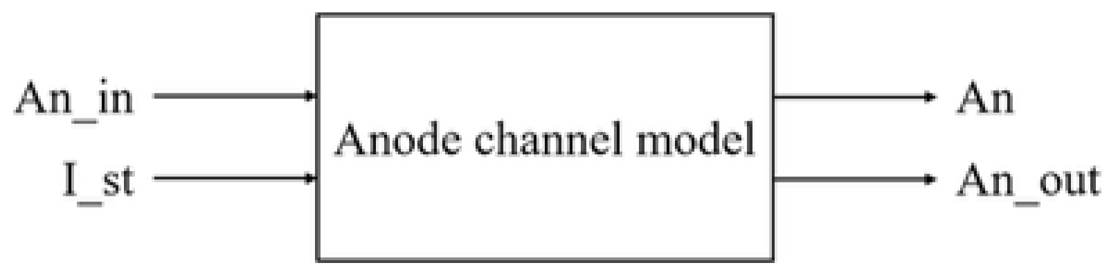
2.4.1. Anode Channel Model

The anode channel model was applied to calculate the anode reactant flow rate, pressure, and temperature of the anode channel and anode channel outlet.

The input and output of the anode channel model are shown in Figure 6.

The gas flow rate of the anode channel is expressed as:

$$W_{\mathrm{a}\mathrm{n}}=W_{\mathrm{a}\mathrm{n},\mathrm{i}\mathrm{n}}-W_{\mathrm{a}\mathrm{n},\mathrm{o}\mathrm{u}\mathrm{t}}-I_{\mathrm{s}\mathrm{t}}\times {\displaystyle \frac{nu{m}_{\mathrm{F}\mathrm{C}}}{2\mathrm{F}}}\times {\mathrm{M}}_{{\mathrm{H}}_2}$$

(11)

where $W_{\mathrm{a}\mathrm{n},\mathrm{o}\mathrm{u}\mathrm{t}}$ is the gas flow rate of the anode outlet, g/s; $nu{m}_{\mathrm{F}\mathrm{C}}$ is the number of single PEMFCs in the stack; $\mathrm{F}=\mathrm{96,485} \mathrm{C}/\mathrm{m}\mathrm{o}\mathrm{l}$ is the Faraday constant; ${\mathrm{M}}_{{\mathrm{H}}_2}=2\mathrm{g}/\mathrm{m}\mathrm{o}\mathrm{l}$ is the mole mass of H₂.

The gas pressure of the anode channel is expressed as:

$$p_{\mathrm{a}\mathrm{n}}={\displaystyle \frac{p_{\mathrm{a}\mathrm{n},\mathrm{i}\mathrm{n}}+p_{\mathrm{a}\mathrm{n},\mathrm{o}\mathrm{u}\mathrm{t}}}{2}}$$

(12)

The gas temperature of the anode channel is expressed as:

$$T_{\mathrm{a}\mathrm{n}}={\displaystyle \frac{T_{\mathrm{a}\mathrm{n},\mathrm{i}\mathrm{n}}+T_{\mathrm{a}\mathrm{n},\mathrm{o}\mathrm{u}\mathrm{t}}}{2}}$$

(13)

The gas flow rate of the anode outlet is expressed as:

$$W_{\mathrm{a}\mathrm{n},\mathrm{o}\mathrm{u}\mathrm{t}}=a_p\times \mathsf{\Delta }{p}_{\mathrm{a}\mathrm{n}}$$

(14)

where $a_p$ is the coefficient between the flow rate and pressure drop, g/s/Pa; $\mathsf{\Delta }{p}_{\mathrm{a}\mathrm{n}}$ is the assumption of anode pressure drop, Pa.

The gas pressure of the anode outlet is expressed as:

$$p_{\mathrm{a}\mathrm{n},\mathrm{o}\mathrm{u}\mathrm{t}}=p_{\mathrm{a}\mathrm{n},\mathrm{i}\mathrm{n}}-\mathsf{\Delta }{p}_{\mathrm{a}\mathrm{n}}$$

(15)

The gas temperature of the anode outlet is expressed as:

$$T_{\mathrm{a}\mathrm{n},\mathrm{o}\mathrm{u}\mathrm{t}}=T_{\mathrm{a}\mathrm{n},\mathrm{i}\mathrm{n}}+\mathsf{\Delta }{T}_{\mathrm{a}\mathrm{n}}$$

(16)

where $\mathsf{\Delta }{T}_{\mathrm{a}\mathrm{n}}$ is the gas temperature rise of the anode channel, K.

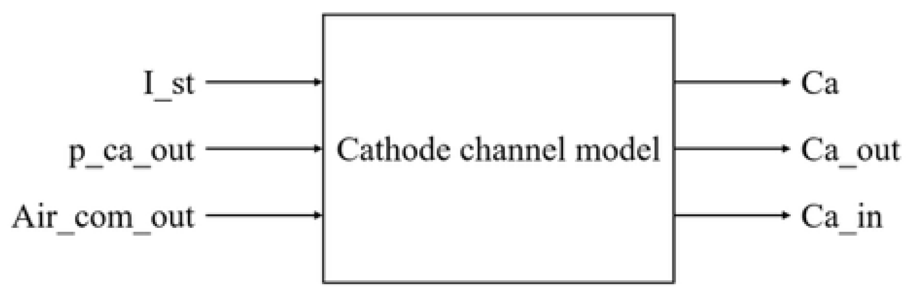
2.4.2. Cathode Channel Model

The cathode channel model was applied to calculate the cathode reactant flow rate, pressure, and temperature of the cathode channel and cathode channel outlet.

The input and output of the cathode channel model are shown in Figure 7.

The gas temperature of the cathode inlet is expressed as:

$$T_{\mathrm{c}\mathrm{a},\mathrm{i}\mathrm{n}}=T_{\mathrm{c}\mathrm{a},\mathrm{c}\mathrm{o}\mathrm{m},\mathrm{o}\mathrm{u}\mathrm{t}}$$

(17)

where $T_{\mathrm{c}\mathrm{a},\mathrm{c}\mathrm{o}\mathrm{m},\mathrm{o}\mathrm{u}\mathrm{t}}$ is the gas temperature of the cathode compressor outlet, K.

The O₂, N₂, and vapor flow rates of the cathode inlet are expressed as:

$$W_{{\mathrm{O}}_2,\mathrm{c}\mathrm{a},\mathrm{i}\mathrm{n}}=x_{{\mathrm{O}}_2,\mathrm{c}\mathrm{a},\mathrm{i}\mathrm{n}}\times W_{\mathrm{a}\mathrm{i}\mathrm{r},\mathrm{c}\mathrm{a},\mathrm{i}\mathrm{n}}$$

(18)

$$W_{{\mathrm{N}}_2,\mathrm{c}\mathrm{a},\mathrm{i}\mathrm{n}}=\left(1-x_{{\mathrm{O}}_2,\mathrm{c}\mathrm{a},\mathrm{i}\mathrm{n}}\right)\times W_{\mathrm{a}\mathrm{i}\mathrm{r},\mathrm{c}\mathrm{a},\mathrm{i}\mathrm{n}}$$

(19)

$$W_{\mathrm{v}\mathrm{a}\mathrm{p}\mathrm{o}\mathrm{r},\mathrm{c}\mathrm{a},\mathrm{i}\mathrm{n}}=W_{\mathrm{c}\mathrm{a},\mathrm{i}\mathrm{n}}-W_{\mathrm{a}\mathrm{i}\mathrm{r},\mathrm{c}\mathrm{a},\mathrm{i}\mathrm{n}}$$

(20)

where $x_{{\mathrm{O}}_2,\mathrm{c}\mathrm{a},\mathrm{i}\mathrm{n}}=\left({\displaystyle \frac{x_{{\mathrm{O}}_2,\mathrm{c}\mathrm{o}\mathrm{m},\mathrm{o}\mathrm{u}\mathrm{t}}}{x_{{\mathrm{O}}_2,\mathrm{c}\mathrm{o}\mathrm{m},\mathrm{o}\mathrm{u}\mathrm{t}}+x_{{\mathrm{N}}_2,\mathrm{c}\mathrm{o}\mathrm{m},\mathrm{o}\mathrm{u}\mathrm{t}}}}\times {\mathrm{M}}_{{\mathrm{O}}_2}\right)/\left({\displaystyle \frac{x_{{\mathrm{O}}_2,\mathrm{c}\mathrm{o}\mathrm{m},\mathrm{o}\mathrm{u}\mathrm{t}}}{x_{{\mathrm{O}}_2,\mathrm{c}\mathrm{o}\mathrm{m},\mathrm{o}\mathrm{u}\mathrm{t}}+x_{{\mathrm{N}}_2,\mathrm{c}\mathrm{o}\mathrm{m},\mathrm{o}\mathrm{u}\mathrm{t}}}}\times {\mathrm{M}}_{{\mathrm{O}}_2}+{\displaystyle \frac{x_{{\mathrm{N}}_2,\mathrm{c}\mathrm{o}\mathrm{m},\mathrm{o}\mathrm{u}\mathrm{t}}}{x_{{\mathrm{O}}_2,\mathrm{c}\mathrm{o}\mathrm{m},\mathrm{o}\mathrm{u}\mathrm{t}}+x_{{\mathrm{N}}_2,\mathrm{c}\mathrm{o}\mathrm{m},\mathrm{o}\mathrm{u}\mathrm{t}}}}\times {\mathrm{M}}_{{\mathrm{N}}_2}\right)$ is the mass fraction of O₂ of cathode inlet, $x_{{\mathrm{N}}_2,\mathrm{c}\mathrm{a},\mathrm{i}\mathrm{n}}=\left({\displaystyle \frac{x_{{\mathrm{N}}_2,\mathrm{c}\mathrm{o}\mathrm{m},\mathrm{o}\mathrm{u}\mathrm{t}}}{x_{{\mathrm{O}}_2,\mathrm{c}\mathrm{o}\mathrm{m},\mathrm{o}\mathrm{u}\mathrm{t}}+x_{{\mathrm{N}}_2,\mathrm{c}\mathrm{o}\mathrm{m},\mathrm{o}\mathrm{u}\mathrm{t}}}}\times {\mathrm{M}}_{{\mathrm{N}}_2}\right)/\left({\displaystyle \frac{x_{{\mathrm{O}}_2,\mathrm{c}\mathrm{o}\mathrm{m},\mathrm{o}\mathrm{u}\mathrm{t}}}{x_{{\mathrm{O}}_2,\mathrm{c}\mathrm{o}\mathrm{m},\mathrm{o}\mathrm{u}\mathrm{t}}+x_{{\mathrm{N}}_2,\mathrm{c}\mathrm{o}\mathrm{m},\mathrm{o}\mathrm{u}\mathrm{t}}}}\times {\mathrm{M}}_{{\mathrm{O}}_2}+{\displaystyle \frac{x_{{\mathrm{N}}_2,\mathrm{c}\mathrm{o}\mathrm{m},\mathrm{o}\mathrm{u}\mathrm{t}}}{x_{{\mathrm{O}}_2,\mathrm{c}\mathrm{o}\mathrm{m},\mathrm{o}\mathrm{u}\mathrm{t}}+x_{{{\mathrm{N}}_2}_{\mathrm{c}\mathrm{o}\mathrm{m},\mathrm{o}\mathrm{u}\mathrm{t}}}}}\times {\mathrm{M}}_{{\mathrm{N}}_2}\right)$ is the mass fraction of N₂ of the cathode inlet, $W_{\mathrm{a}\mathrm{i}\mathrm{r},\mathrm{c}\mathrm{a},\mathrm{i}\mathrm{n}}={\mathrm{W}}_{\mathrm{c}\mathrm{a},\mathrm{i}\mathrm{n}}/\left({\displaystyle \frac{R{H}_{\mathrm{c}\mathrm{a},\mathrm{i}\mathrm{n}}\ast LUT\left(p\right)}{p_{\mathrm{c}\mathrm{a},\mathrm{i}\mathrm{n}}-R{H}_{\mathrm{c}\mathrm{a},\mathrm{i}\mathrm{n}}\ast LUT\left(p\right)}}\times {\displaystyle \frac{{\mathrm{M}}_{{\mathrm{H}}_2\mathrm{O}}}{{\mathrm{M}}_{\mathrm{a}\mathrm{i}\mathrm{r}}}}+1\right)$ is the air flow rate of cathode inlet, g/s.

The O₂ pressure of the cathode inlet is expressed as:

$$p_{{\mathrm{O}}_2,\mathrm{c}\mathrm{a},\mathrm{i}\mathrm{n}}=\left[p_{\mathrm{c}\mathrm{a},\mathrm{i}\mathrm{n}}-R{H}_{\mathrm{c}\mathrm{a},\mathrm{i}\mathrm{n}}\times LUT\left(T_{\mathrm{c}\mathrm{a},\mathrm{c}\mathrm{o}\mathrm{m},\mathrm{o}\mathrm{u}\mathrm{t}}\right)\right]\times x_{{\mathrm{O}}_2,\mathrm{c}\mathrm{o}\mathrm{m},\mathrm{o}\mathrm{u}\mathrm{t}}$$

(21)

where $LUT\left(T_{\mathrm{c}\mathrm{a},\mathrm{c}\mathrm{o}\mathrm{m},\mathrm{o}\mathrm{u}\mathrm{t}}\right)$ is the relationship between the saturated vapor pressure and gas temperature of the compressor outlet.

The O₂, N₂, and vapor flow rates of the cathode outlet were similar to those of cathode inlet. The gas temperature of the cathode outlet is expressed as:

$$T_{\mathrm{c}\mathrm{a},\mathrm{o}\mathrm{u}\mathrm{t}}=T_{\mathrm{s}\mathrm{t}}$$

(22)

The O₂, N₂, and vapor flow rates of the cathode outlet are expressed as:

$$W_{{\mathrm{O}}_2,\mathrm{c}\mathrm{a},\mathrm{o}\mathrm{u}\mathrm{t}}=x_{{\mathrm{O}}_2,\mathrm{c}\mathrm{a},\mathrm{o}\mathrm{u}\mathrm{t}}\times W_{\mathrm{a}\mathrm{i}\mathrm{r},\mathrm{c}\mathrm{a},\mathrm{o}\mathrm{u}\mathrm{t}}$$

(23)

$$W_{{\mathrm{N}}_2,\mathrm{c}\mathrm{a},\mathrm{o}\mathrm{u}\mathrm{t}}=\left(1-x_{{\mathrm{O}}_2,\mathrm{c}\mathrm{a},\mathrm{o}\mathrm{u}\mathrm{t}}\right)\times W_{\mathrm{a}\mathrm{i}\mathrm{r},\mathrm{c}\mathrm{a},\mathrm{o}\mathrm{u}\mathrm{t}}$$

(24)

$$W_{\mathrm{v}\mathrm{a}\mathrm{p}\mathrm{o}\mathrm{r},\mathrm{c}\mathrm{a},\mathrm{o}\mathrm{u}\mathrm{t}}=W_{\mathrm{c}\mathrm{a},\mathrm{i}\mathrm{n}}-W_{\mathrm{a}\mathrm{i}\mathrm{r},\mathrm{c}\mathrm{a},\mathrm{o}\mathrm{u}\mathrm{t}}$$

(25)

where $x_{{\mathrm{O}}_2,\mathrm{c}\mathrm{a},\mathrm{o}\mathrm{u}\mathrm{t}}=\left({\displaystyle \frac{x_{{\mathrm{O}}_2,\mathrm{c}\mathrm{a}}}{x_{{\mathrm{O}}_2,\mathrm{c}\mathrm{a}}+x_{{\mathrm{N}}_2,\mathrm{c}\mathrm{a}}}}\times {\mathrm{M}}_{{\mathrm{O}}_2}\right)/\left({\displaystyle \frac{x_{{\mathrm{O}}_2,\mathrm{c}\mathrm{a}}}{x_{{\mathrm{O}}_2,\mathrm{c}\mathrm{a}}+x_{{\mathrm{N}}_2,\mathrm{c}\mathrm{a}}}}\times {\mathrm{M}}_{{\mathrm{O}}_2}+{\displaystyle \frac{x_{{\mathrm{N}}_2,\mathrm{c}\mathrm{a}}}{x_{{\mathrm{O}}_2,\mathrm{c}\mathrm{a}}+x_{{\mathrm{N}}_2,\mathrm{c}\mathrm{a}}}}\times {\mathrm{M}}_{{\mathrm{N}}_2}\right)$ is the mass fraction of O₂ of the cathode outlet, $x_{{\mathrm{N}}_2,\mathrm{c}\mathrm{a},\mathrm{o}\mathrm{u}\mathrm{t}}=\left({\displaystyle \frac{x_{{\mathrm{N}}_2,\mathrm{c}\mathrm{a}}}{x_{{\mathrm{O}}_2,\mathrm{c}\mathrm{a}}+x_{{\mathrm{N}}_2,\mathrm{c}\mathrm{a}}}}\times {\mathrm{M}}_{{\mathrm{N}}_2}\right)/\left({\displaystyle \frac{x_{{\mathrm{O}}_2,\mathrm{c}\mathrm{a}}}{x_{{\mathrm{O}}_2,\mathrm{c}\mathrm{a}}+x_{{\mathrm{N}}_2,\mathrm{c}\mathrm{a}}}}\times {\mathrm{M}}_{{\mathrm{O}}_2}+{\displaystyle \frac{x_{{\mathrm{N}}_2,\mathrm{c}\mathrm{a}}}{x_{{\mathrm{O}}_2,\mathrm{c}\mathrm{a}}+x_{{\mathrm{N}}_2,\mathrm{c}\mathrm{a}}}}\times {\mathrm{M}}_{{\mathrm{N}}_2}\right)$ is the mass fraction of N₂ of the cathode outlet, $W_{\mathrm{a}\mathrm{i}\mathrm{r},\mathrm{c}\mathrm{a},\mathrm{o}\mathrm{u}\mathrm{t}}=W_{\mathrm{c}\mathrm{a},\mathrm{t}\mathrm{h},\mathrm{o}\mathrm{u}\mathrm{t}}/\left({\displaystyle \frac{R{H}_{\mathrm{c}\mathrm{a}}\times LUT\left(T_{\mathrm{c}\mathrm{a},\mathrm{o}\mathrm{u}\mathrm{t}}\right)}{p_{\mathrm{c}\mathrm{a},\mathrm{o}\mathrm{u}\mathrm{t}}-R{H}_{\mathrm{c}\mathrm{a}}\times LUT\left(T_{\mathrm{c}\mathrm{a},\mathrm{o}\mathrm{u}\mathrm{t}}\right)}}\times {\displaystyle \frac{{\mathrm{M}}_{{\mathrm{H}}_2\mathrm{O}}}{{\mathrm{M}}_{\mathrm{a}\mathrm{i}\mathrm{r}}}}+1\right)$ is the air flow rate of the cathode inlet, g/s; $W_{\mathrm{c}\mathrm{a},\mathrm{t}\mathrm{h},\mathrm{o}\mathrm{u}\mathrm{t}}=k_{\mathrm{t}\mathrm{h}}\mathrm{\ast }\left(p_{\mathrm{c}\mathrm{a}}-p_{\mathrm{c}\mathrm{a},\mathrm{o}\mathrm{u}\mathrm{t}}\right)$ is the gas flow rate of the throttle outlet, g/s.

The O₂ pressure of the cathode inlet is expressed as:

$$p_{{\mathrm{O}}_2,\mathrm{c}\mathrm{a},\mathrm{i}\mathrm{n}}=\left[p_{\mathrm{c}\mathrm{a},\mathrm{i}\mathrm{n}}-R{H}_{\mathrm{c}\mathrm{a},\mathrm{i}\mathrm{n}}\times LUT\left(p\right)\right]\times x_{{\mathrm{O}}_2,\mathrm{c}\mathrm{o}\mathrm{m},\mathrm{o}\mathrm{u}\mathrm{t}}$$

(26)

where $LUT\left(p\right)$ is the relationship between the saturated vapor pressure and gas temperature of the compressor outlet.

The O₂ flow rate and pressure of the cathode channel are expressed as:

$$W_{\mathrm{c}\mathrm{a},{\mathrm{O}}_2}=W_{\mathrm{c}\mathrm{a},{\mathrm{O}}_2,\mathrm{i}\mathrm{n}}-W_{\mathrm{c}\mathrm{a},{\mathrm{O}}_2,\mathrm{o}\mathrm{u}\mathrm{t}}-W_{\mathrm{c}\mathrm{a},{\mathrm{O}}_2,\mathrm{r}\mathrm{e}\mathrm{a}\mathrm{c}\mathrm{t}\mathrm{e}\mathrm{d}}$$

(27)

$$p_{\mathrm{c}\mathrm{a},{\mathrm{O}}_2}={\displaystyle \frac{\int W_{\mathrm{c}\mathrm{a},{\mathrm{O}}_2}dt\times R\times T_{\mathrm{c}\mathrm{a}}}{{\mathrm{M}}_{{\mathrm{O}}_2}\times V{o}_{\mathrm{c}\mathrm{a}}}}$$

(28)

The N₂ pressure of the cathode channel is expressed as:

$$p_{\mathrm{c}\mathrm{a},{\mathrm{N}}_2}={\displaystyle \frac{\int W_{\mathrm{c}\mathrm{a},{\mathrm{N}}_2}dt\times R\times T_{\mathrm{c}\mathrm{a}}}{{\mathrm{M}}_{{\mathrm{N}}_2}\times V{o}_{\mathrm{c}\mathrm{a}}}}$$

(29)

where $W_{\mathrm{c}\mathrm{a},{\mathrm{N}}_2}=W_{\mathrm{c}\mathrm{a},{\mathrm{N}}_2,\mathrm{i}\mathrm{n}}-W_{\mathrm{c}\mathrm{a},{\mathrm{N}}_2,\mathrm{o}\mathrm{u}\mathrm{t}}$ is the N₂ flow rate of the cathode channel, g/s.

The vapor pressure of the cathode channel is expressed as:

$$p_{\mathrm{c}\mathrm{a},\mathrm{v}\mathrm{a}\mathrm{p}\mathrm{o}\mathrm{r}}={\displaystyle \frac{\int W_{\mathrm{c}\mathrm{a},\mathrm{v}\mathrm{a}\mathrm{p}\mathrm{o}\mathrm{r}}dt\times R\times T_{\mathrm{c}\mathrm{a}}}{{\mathrm{M}}_{{\mathrm{H}}_2\mathrm{O}}\times V{o}_{\mathrm{c}\mathrm{a}}}}$$

(30)

where $W_{\mathrm{c}\mathrm{a},\mathrm{v}\mathrm{a}\mathrm{p}\mathrm{o}\mathrm{r}}=W_{\mathrm{c}\mathrm{a},\mathrm{v}\mathrm{a}\mathrm{p}\mathrm{o}\mathrm{r},\mathrm{i}\mathrm{n}}-W_{\mathrm{c}\mathrm{a},\mathrm{v}\mathrm{a}\mathrm{p}\mathrm{o}\mathrm{r},\mathrm{o}\mathrm{u}\mathrm{t}}-LUT\left(I_{\mathrm{s}\mathrm{t}}\right)+W_{\mathrm{c}\mathrm{a},\mathrm{v}\mathrm{a}\mathrm{p}\mathrm{o}\mathrm{r},\mathrm{g}\mathrm{e}\mathrm{n}\mathrm{e}\mathrm{r}\mathrm{a}\mathrm{t}\mathrm{e}\mathrm{d}}$ is the vapor flow rate of the cathode channel, g/s.

The vapor flow rate of the cathode channel is expressed as:

$$W_{\mathrm{c}\mathrm{a},\mathrm{v}\mathrm{a}\mathrm{p}\mathrm{o}\mathrm{r},\mathrm{g}\mathrm{e}\mathrm{n}\mathrm{e}\mathrm{r}\mathrm{a}\mathrm{t}\mathrm{e}\mathrm{d}}=I_{\mathrm{s}\mathrm{t}}\times {\displaystyle \frac{nu{m}_{\mathrm{F}\mathrm{C}}}{2\mathrm{F}}}\times {\mathrm{M}}_{{\mathrm{H}}_2\mathrm{O}}$$

(31)

The reacted O₂ flow rate is expressed as:

$$W_{\mathrm{c}\mathrm{a},{\mathrm{O}}_2,\mathrm{r}\mathrm{e}\mathrm{a}\mathrm{c}\mathrm{t}\mathrm{e}\mathrm{d}}=I_{\mathrm{s}\mathrm{t}}\times {\displaystyle \frac{nu{m}_{\mathrm{F}\mathrm{C}}}{4\mathrm{F}}}\times {\mathrm{M}}_{{\mathrm{O}}_2}$$

(32)

The total pressure of the cathode channel is expressed as:

$$p_{\mathrm{c}\mathrm{a}}=p_{\mathrm{c}\mathrm{a},{\mathrm{O}}_2}+p_{\mathrm{c}\mathrm{a},{\mathrm{N}}_2}+p_{\mathrm{c}\mathrm{a},\mathrm{v}\mathrm{a}\mathrm{p}\mathrm{o}\mathrm{r}}$$

(33)

The mole fractions of O₂, N₂, and vapor are expressed as:

$$x_{\mathrm{c}\mathrm{a},{\mathrm{O}}_2}={\displaystyle \frac{p_{\mathrm{c}\mathrm{a},{\mathrm{O}}_2}}{p_{\mathrm{c}\mathrm{a}}}}$$

(34)

$$x_{\mathrm{c}\mathrm{a},{\mathrm{N}}_2}={\displaystyle \frac{p_{\mathrm{c}\mathrm{a},{\mathrm{N}}_2}}{p_{\mathrm{c}\mathrm{a}}}}$$

(35)

$$x_{\mathrm{c}\mathrm{a},\mathrm{v}\mathrm{a}\mathrm{p}\mathrm{o}\mathrm{r}}={\displaystyle \frac{p_{\mathrm{c}\mathrm{a},\mathrm{v}\mathrm{a}\mathrm{p}\mathrm{o}\mathrm{r}}}{p_{\mathrm{c}\mathrm{a}}}}$$

(36)

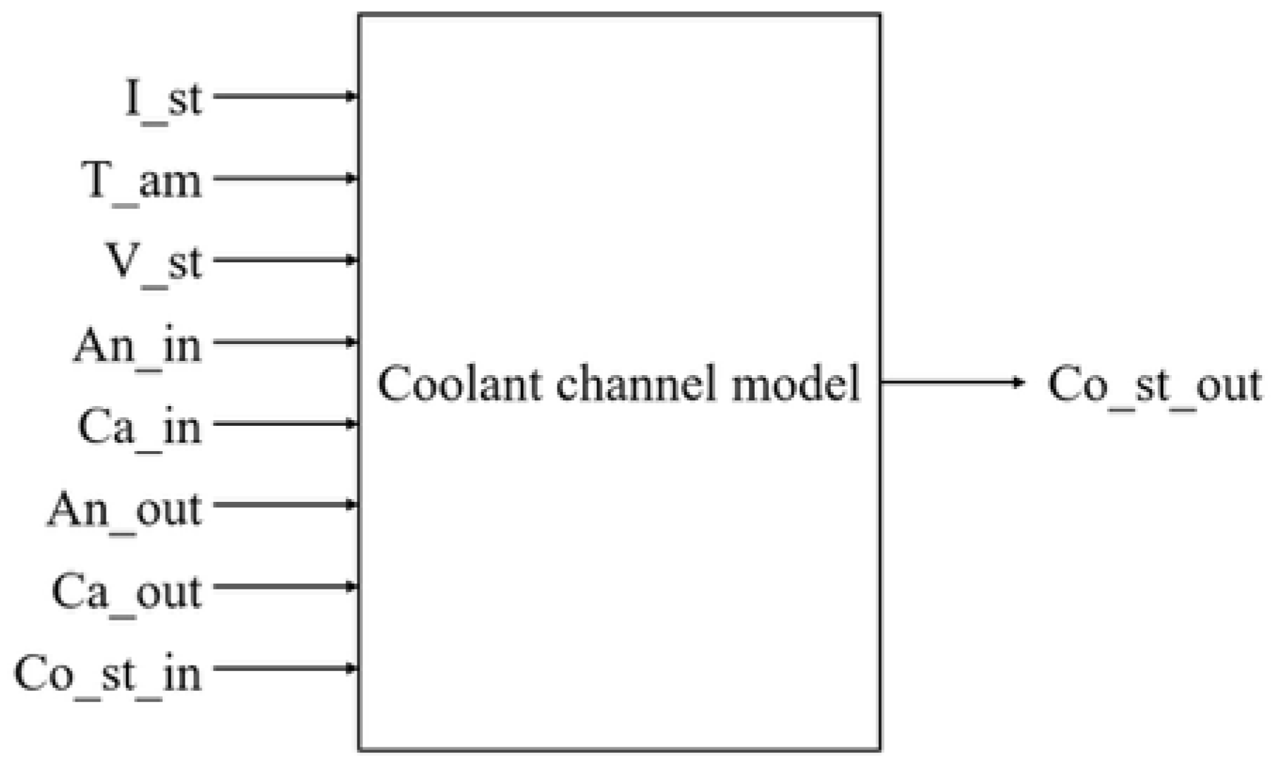
2.4.3. Coolant Channel Model

The coolant channel model was applied to calculate the stack temperature. The input and output of the coolant channel model are shown in Figure 8. The input of this model was the loading current of stack, temperature of ambient, voltage of stack, gas flow rate and temperature of the anode/cathode inlet and outlet, and coolant flow rate and temperature of the stack inlet. The output was the coolant flow rate and temperature of the stack outlet.

The PEMFC stack temperature determined by four parts, including the heat generation, natural convection, radiative convection, and forced convection (radiator heat dissipation) of stack, is expressed as:

$${\dot{Q}}_{\mathrm{s}\mathrm{t}}={\dot{Q}}_{\mathrm{a}\mathrm{d}\mathrm{d}}-{\dot{Q}}_{\mathrm{c}\mathrm{o}\mathrm{n}\mathrm{v},\mathrm{n}\mathrm{a}}-{\dot{Q}}_{\mathrm{c}\mathrm{o}\mathrm{n}\mathrm{v},\mathrm{r}\mathrm{a}\mathrm{d}}-{\dot{Q}}_{\mathrm{c}\mathrm{o}\mathrm{n}\mathrm{v},\mathrm{f}\mathrm{o}}$$

(37)

where ${\dot{Q}}_{\mathrm{a}\mathrm{d}\mathrm{d}}$ is the stack thermal power, W; ${\dot{Q}}_{\mathrm{c}\mathrm{o}\mathrm{n}\mathrm{v},\mathrm{n}\mathrm{a}}$ is the thermal power of natural convection, W; ${\dot{Q}}_{\mathrm{c}\mathrm{o}\mathrm{n}\mathrm{v},\mathrm{r}\mathrm{a}\mathrm{d}}$ is the thermal power of radiative convection, W; ${\dot{Q}}_{\mathrm{c}\mathrm{o}\mathrm{n}\mathrm{v},\mathrm{f}\mathrm{o}}$ is the thermal power of forced convection, W.

The stack temperature is expressed as:

$${\dot{Q}}_{\mathrm{s}\mathrm{t}}=c_{\mathrm{s}\mathrm{t}}\times m_{\mathrm{s}\mathrm{t}}\times {\displaystyle \frac{d{T}_{\mathrm{s}\mathrm{t}}}{dt}}$$

(38)

where $c_{\mathrm{s}\mathrm{t}}$ is the specific heat capacity of stack, J/g/K; $m_{\mathrm{s}\mathrm{t}}$ is the mass of stack, g.

The stack thermal power is expressed as:

$${\dot{Q}}_{\mathrm{a}\mathrm{d}\mathrm{d}}=\left(nu{m}_{\mathrm{F}\mathrm{C}}\times E_{\mathrm{n}\mathrm{e}\mathrm{r}\mathrm{n}\mathrm{s}\mathrm{t}}-V_{\mathrm{s}\mathrm{t}}\right)\times I_{\mathrm{s}\mathrm{t}}+\left({\dot{Q}}_{\mathrm{r}\mathrm{e},\mathrm{i}\mathrm{n}}-{\dot{Q}}_{\mathrm{r}\mathrm{e},\mathrm{o}\mathrm{u}\mathrm{t}}\right)$$

(39)

where $E_{\mathrm{n}\mathrm{e}\mathrm{r}\mathrm{n}\mathrm{s}\mathrm{t}}=1.481 \mathrm{V}$ is the Nernst voltage; $V_{\mathrm{s}\mathrm{t}}$ is the voltage of stack, V; ${\dot{Q}}_{\mathrm{r}\mathrm{e},\mathrm{i}\mathrm{n}}$ is the heat power of inlet reactant, W; ${\dot{Q}}_{\mathrm{r}\mathrm{e},\mathrm{o}\mathrm{u}\mathrm{t}}$ is the heat power of outlet reactant, W.

The heat power of the inlet reactant is expressed as:

$${\dot{Q}}_{\mathrm{r}\mathrm{e},\mathrm{i}\mathrm{n}}=\left(c_{{\mathrm{O}}_2}\times W_{\mathrm{c}\mathrm{a},{\mathrm{O}}_2,\mathrm{i}\mathrm{n}}+c_{{\mathrm{N}}_2}\times W_{\mathrm{c}\mathrm{a},{\mathrm{N}}_2,\mathrm{i}\mathrm{n}}+c_{\mathrm{v}\mathrm{a}\mathrm{p}\mathrm{o}\mathrm{r}}\times W_{\mathrm{c}\mathrm{a},\mathrm{v}\mathrm{a}\mathrm{p}\mathrm{o}\mathrm{r},\mathrm{i}\mathrm{n}}\right)\left(T_{\mathrm{c}\mathrm{a},\mathrm{i}\mathrm{n}}-T_{\mathrm{a}\mathrm{m}}\right)+c_{{\mathrm{H}}_2}\times W_{\mathrm{a}\mathrm{n},{\mathrm{H}}_2,\mathrm{i}\mathrm{n}}\times \left(T_{\mathrm{a}\mathrm{n},\mathrm{i}\mathrm{n}}-T_{\mathrm{a}\mathrm{m}}\right)$$

(40)

where $c_{{\mathrm{O}}_2}$ is the specific heat capacity of O₂, J/g/K; $W_{\mathrm{c}\mathrm{a},{\mathrm{O}}_2,\mathrm{i}\mathrm{n}}$ is the O₂ flow rate of the cathode inlet, g/s; $c_{{\mathrm{N}}_2}$ is the specific heat capacity of N₂, J/g/K; $W_{\mathrm{c}\mathrm{a},{\mathrm{N}}_2,\mathrm{i}\mathrm{n}}$ is the N₂ flow rate of the cathode inlet, g/s; $c_{\mathrm{v}\mathrm{a}\mathrm{p}\mathrm{o}\mathrm{r}}$ is the specific heat capacity of vapor, J/g/K; $W_{\mathrm{c}\mathrm{a},\mathrm{v}\mathrm{a}\mathrm{p}\mathrm{o}\mathrm{r},\mathrm{i}\mathrm{n}}$ is the vapor flow rate of the cathode inlet, g/s; $T_{\mathrm{c}\mathrm{a},\mathrm{i}\mathrm{n}}$ is the gas temperature of the cathode inlet, K; $c_{{\mathrm{H}}_2}$ is the specific heat capacity of H₂, J/g/K; $W_{\mathrm{a}\mathrm{n},{\mathrm{H}}_2,\mathrm{i}\mathrm{n}}$ is the H₂ flow rate of the anode inlet, g/s.

The heat power of the outlet reactant is expressed as:

$${\dot{Q}}_{\mathrm{r}\mathrm{e},\mathrm{o}\mathrm{u}\mathrm{t}}=\left(c_{{\mathrm{O}}_2}\times W_{\mathrm{c}\mathrm{a},{\mathrm{O}}_2,\mathrm{o}\mathrm{u}\mathrm{t}}+c_{{\mathrm{N}}_2}\times W_{\mathrm{c}\mathrm{a},{\mathrm{N}}_2,\mathrm{o}\mathrm{u}\mathrm{t}}+c_{\mathrm{v}\mathrm{a}\mathrm{p}\mathrm{o}\mathrm{r}}\times W_{\mathrm{c}\mathrm{a},\mathrm{v}\mathrm{a}\mathrm{p}\mathrm{o}\mathrm{r},\mathrm{o}\mathrm{u}\mathrm{t}}+c_{{\mathrm{H}}_2}\times W_{\mathrm{a}\mathrm{n},{\mathrm{H}}_2,\mathrm{o}\mathrm{u}\mathrm{t}}\right)\times \left(T_{\mathrm{s}\mathrm{t}}-T_{\mathrm{a}\mathrm{m}}\right)$$

(41)

where $W_{\mathrm{c}\mathrm{a},{\mathrm{O}}_2,\mathrm{o}\mathrm{u}\mathrm{t}}$ is the O₂ flow rate of the cathode outlet, g/s; $W_{\mathrm{c}\mathrm{a},{\mathrm{N}}_2,\mathrm{o}\mathrm{u}\mathrm{t}}$ is the N₂ flow rate of the cathode outlet, g/s;$W_{\mathrm{c}\mathrm{a},\mathrm{v}\mathrm{a}\mathrm{p}\mathrm{o}\mathrm{r},\mathrm{o}\mathrm{u}\mathrm{t}}$ is the vapor flow rate of the cathode outlet, g/s;$W_{\mathrm{c}\mathrm{a},{\mathrm{H}}_2,\mathrm{o}\mathrm{u}\mathrm{t}}$ is the H₂ flow rate of the anode outlet, g/s.

The thermal power of natural convection is expressed as:

$${\dot{Q}}_{\mathrm{c}\mathrm{o}\mathrm{n}\mathrm{v},\mathrm{n}\mathrm{a}}=h_{\mathrm{s}\mathrm{t}}\times A_{\mathrm{s}\mathrm{t},\mathrm{e}\mathrm{x}\mathrm{t}\mathrm{e}\mathrm{r}\mathrm{i}\mathrm{o}\mathrm{r}}\times \left(T_{\mathrm{s}\mathrm{t}}-T_{\mathrm{a}\mathrm{m}}\right)$$

(42)

where $h_{\mathrm{s}\mathrm{t}}$ is the convective heat transfer coefficient, $\mathrm{W}/({\mathrm{m}}^2·\mathrm{K})$; $A_{\mathrm{s}\mathrm{t},\mathrm{e}\mathrm{x}\mathrm{t}\mathrm{e}\mathrm{r}\mathrm{i}\mathrm{o}\mathrm{r}}$ is the external surface area of the stack, m².

The thermal power of radiative convection is expressed as:

$${\dot{Q}}_{\mathrm{c}\mathrm{o}\mathrm{n}\mathrm{v},\mathrm{r}\mathrm{a}\mathrm{d}}=A_{\mathrm{s}\mathrm{t},\mathrm{e}\mathrm{x}\mathrm{t}\mathrm{e}\mathrm{r}\mathrm{i}\mathrm{o}\mathrm{r}}\times 0.85\times 5.67\times {10}^{-8}\times \left(T_{\mathrm{s}\mathrm{t}}^4-T_{\mathrm{a}\mathrm{m}}^4\right)$$

(43)

The thermal power of forced convection is expressed as:

$${\dot{Q}}_{\mathrm{c}\mathrm{o}\mathrm{n}\mathrm{v},\mathrm{f}\mathrm{o}}=c_{\mathrm{c}\mathrm{o}}\times W_{\mathrm{c}\mathrm{o},\mathrm{s}\mathrm{t},\mathrm{i}\mathrm{n}}\times \left(T_{\mathrm{s}\mathrm{t}}-T_{\mathrm{c}\mathrm{o},\mathrm{s}\mathrm{t},\mathrm{i}\mathrm{n}}\right)$$

(44)

where $W_{\mathrm{c}\mathrm{o},\mathrm{s}\mathrm{t},\mathrm{i}\mathrm{n}}$ is the coolant flow rate of the stack inlet, g/s; $T_{\mathrm{c}\mathrm{o},\mathrm{s}\mathrm{t},\mathrm{i}\mathrm{n}}$ is the coolant temperature of the stack inlet, K.

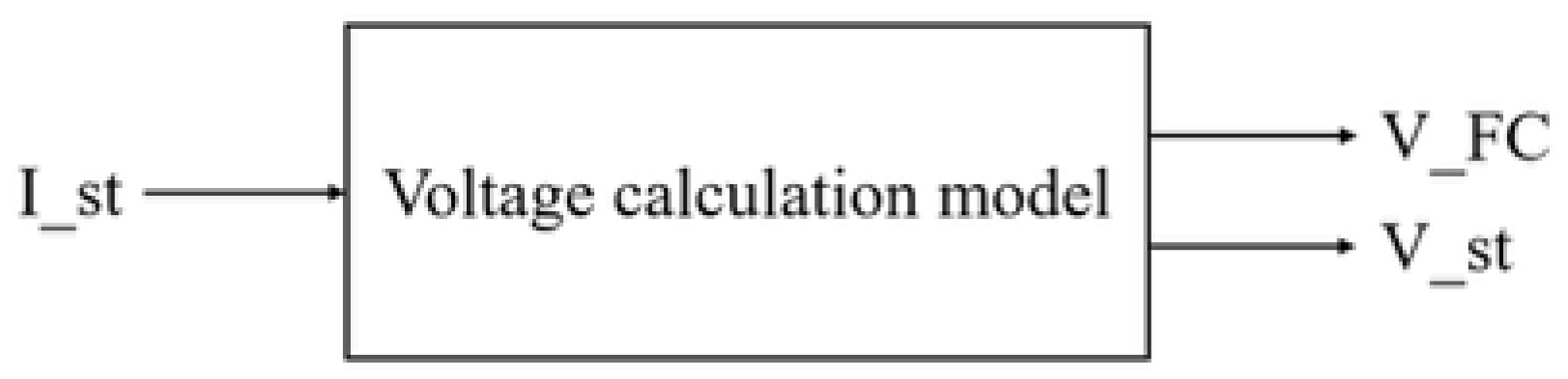
2.4.4. Voltage Calculation Model

The voltage calculation model was applied to transfer the operating time of the loading current to the operating time of the standard current (70 A in this study) and calculate the output voltage with the operation time.

The input and output of the voltage calculation model are shown in Figure 9.

First, the current transformation model will transfer the operating time of the loading current to the operating time of the standard current (70 A in this study) according to the equivalent coefficient between the loading current and standard current, which is expressed as:

$$t_{\mathrm{s}\mathrm{t}\mathrm{a}\mathrm{n}\mathrm{d}\mathrm{a}\mathrm{r}\mathrm{d}}=t\times LUT\left(I_{\mathrm{s}\mathrm{t}}\left(t\right)/70\right)$$

(45)

where $t$ is the operating time of the loading current of the stack, s; $LUT\left(I_{\mathrm{s}\mathrm{t}}\left(t\right)/70\right)$ is the equivalent coefficient between the loading current and standard current.

Second, the voltage of the stack under the standard current is calculated:

$$V_{\mathrm{F}\mathrm{C},\mathrm{s}\mathrm{t}\mathrm{a}\mathrm{n}\mathrm{d}\mathrm{a}\mathrm{r}\mathrm{d}}\left(t\right)=V_{\mathrm{F}\mathrm{C},\mathrm{s}\mathrm{t}\mathrm{a}\mathrm{n}\mathrm{d}\mathrm{a}\mathrm{r}\mathrm{d}}\left(0\right)\times LUT\left(t_{\mathrm{s}\mathrm{t}\mathrm{a}\mathrm{n}\mathrm{d}\mathrm{a}\mathrm{r}\mathrm{d}}\right)$$

(46)

where $V_{\mathrm{F}\mathrm{C},\mathrm{s}\mathrm{t}\mathrm{a}\mathrm{n}\mathrm{d}\mathrm{a}\mathrm{r}\mathrm{d}}\left(0\right)$ is the voltage under the standard current at time 0, V; $LUT\left(t_{\mathrm{s}\mathrm{t}\mathrm{a}\mathrm{n}\mathrm{d}\mathrm{a}\mathrm{r}\mathrm{d}}\right)$ is the relationship between the operating time under the standard current and voltage degradation coefficient.

Finally, the output voltages of a single FC and stack under the loading current are expressed as:

$$V_{\mathrm{F}\mathrm{C}}\left(t\right)=I_{\mathrm{s}\mathrm{t}\mathrm{a}\mathrm{r}\mathrm{d}\mathrm{a}\mathrm{r}\mathrm{d}}\times V_{\mathrm{F}\mathrm{C},\mathrm{s}\mathrm{t}\mathrm{a}\mathrm{n}\mathrm{d}\mathrm{a}\mathrm{r}\mathrm{d}}\left(t\right)/I_{\mathrm{s}\mathrm{t}}\left(t\right)$$

(47)

$$V_{\mathrm{s}\mathrm{t}}\left(t\right)=V_{\mathrm{F}\mathrm{C}}\left(t\right)\times nu{m}_{\mathrm{F}\mathrm{C}}$$

(48)

3. Control Framework Design Based on the Degraded PEMFC

There are two parts including the designs of the ECU and FCU.

3.1. ECU Design

The ECU shown in Figure 10 consisted of five parts including the system on/off, RUL, SoH, demand current determination, and ambient information modules. Moreover, the function of the ECU is to determine the demand power according to the information from the feedback of the CAN, RUL, SoH, and some ambient information.

3.1.1. System On/Off Module

The function of the system on/off module is to start or stop the system of the PEMFC.

3.1.2. RUL Module

The function of the RUL module is to provide a signal of the state of the FC (Normal, Repair, and Replace) and determine the estimated duration of the SoH. This module operates once per 100 h, and the output of this module is the prediction of the RUL. Furthermore, the estimated duration of the SoH was selected according to the prediction of the RUL. If the prediction of the RUL is less than 350 h, the estimated duration of the SoH is 5 h. If the prediction of the RUL is greater than 350 h and less than 500 h, the estimated duration of the SoH is 10 h. If the prediction of the RUL is greater than 500 h, the estimated duration of the SoH is 20 h. Meanwhile, if the prediction of the RUL is greater than 500 h, the state of the FC shows “Normal”. If the prediction of the RUL is greater than 200 h and less than 500 h, the state of FC shows “Repair”. If the prediction of the RUL is less than 200 h, the state of FC shows “Replace” [16].

3.1.3. SoH Module

The function of the SoH module is to predict the output power of the PEMFC according to the historical information of PEMFC operation and decide whether to update the feedforward table of the FCU. The operating frequency of this module is dependent on the prediction of the RUL, and the output of this module is LUT selection and the SoH. Furthermore, if the prediction of the RUL is greater than 500 h, the LUT selection is LUT1. If the prediction of the RUL is greater than 200 h and less than 500 h, the LUT selection is LUT2. If the prediction of the RUL is less than 200 h, the LUT selection is LUT3 [1,17].

3.1.4. Current Determination Module

The function of the current determination module is to determine the demand current according to the information from the feedback of the CAN, RUL, SoH, and operating mode. First, there are two kinds of operating modes including the constant current (power reduction) and constant power (current rise) outputs. The current of the constant current output is 70 A, and that of the constant power output is obtained by $LUT\_P-I\left(t\right)$.

3.1.5. Ambient Information Perception Module

The function of the ambient information perception module is providing several ambient information including the temperature, pressure, and RH.

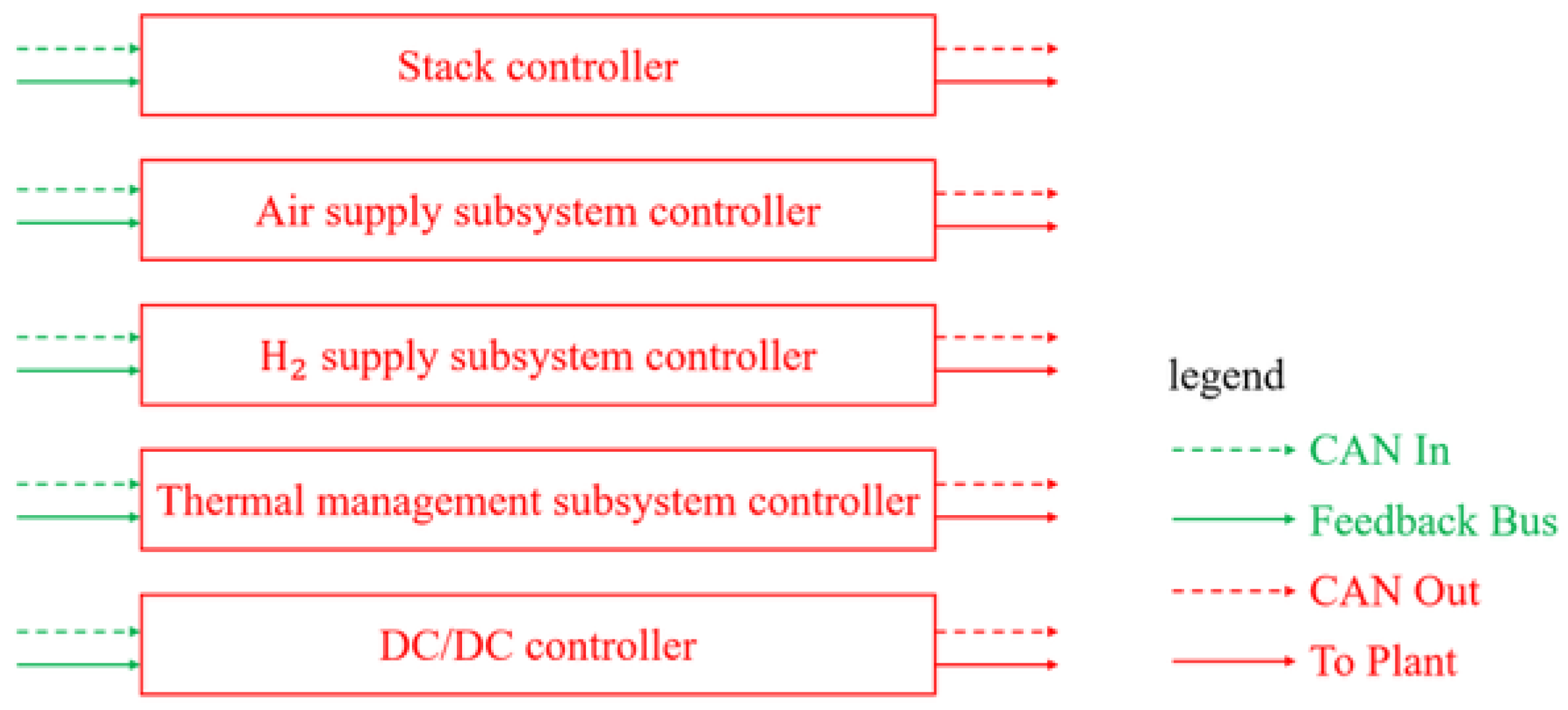
3.2. FCU Design

The FCU shown in Figure 11 consisted of five parts including the stack controllers, air supply subsystem, H₂ supply subsystem, thermal management subsystem, and DC/DC. Furthermore, the function of the FCU is to provide the control signal to each actuator according to the information from the CAN In and Feedback Bus.

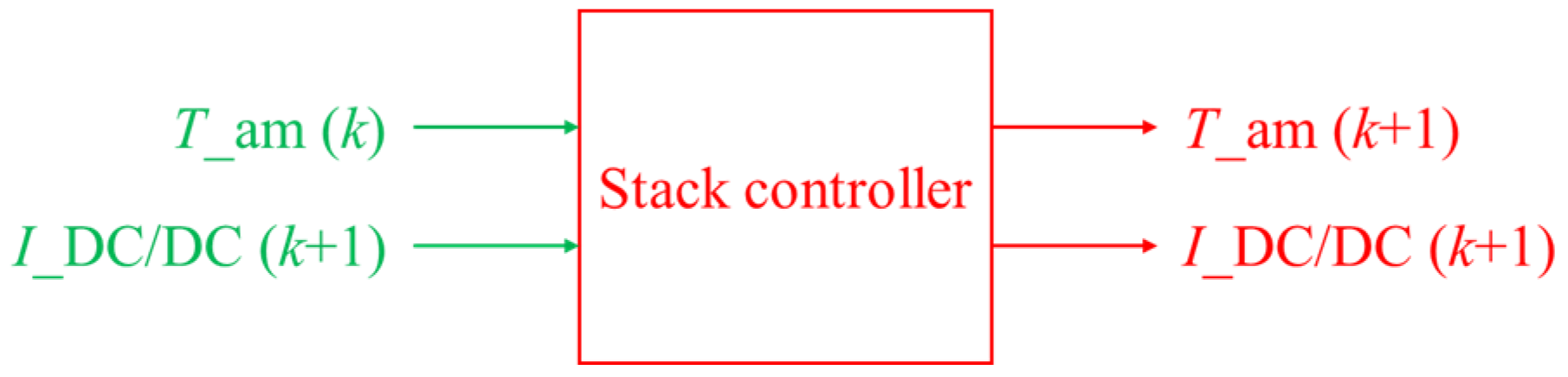
3.2.1. Stack Controller

The stack controller shown in Figure 12 provides the ambient temperature and loading current of the DC/DC to the CAN Out and stack module.

The ambient temperature of the CAN Out and stack module is expressed as:

$$T_{am}(k+1)=T_{am}\left(k\right)$$

(49)

The loading current of the DC/DC of the CAN Out and stack module from the DC/DC controller is expressed as:

$$I_{DC/DC}(k+1)=I_{DC/DC}(k+1)$$

(50)

3.2.2. Air Supply Subsystem Controller

The air supply subsystem controller shown in Figure 13 provides the ambient temperature and pressure, compressor speed, and throttle opening to the CAN Out and air supply subsystem module.

The ambient temperature and pressure, compressor speed, and throttle opening of the CAN Out and air supply subsystem module are expressed as:

$$T_{am}(k+1)=T_{am}\left(k\right)$$

(51)

$$p_{am}(k+1)=p_{am}\left(k\right)$$

(52)

$$n_{com}(k+1)=LUT\_n_{com}\left(I_{DC/DC}\right)+K_p\_n_{com}\times e\_n_{com}(k+1)$$

(53)

$$ph{i}_{th}(k+1)=LUT\_ph{i}_{th}\left(I_{DC/DC}\right)+K_p\_ph{i}_{th}\times e\_ph{i}_{th}(k+1)$$

(54)

where $LUT\_n_{com}\left(I_{DC/DC}\right),K_p\_n_{com},e\_n_{com}(k+1)=LUT\_n_{com}\left(I_{DC/DC}\right)-n_{com,ac}\left(k\right)$ are the feedforward table, proportional, and difference of the compressor speed, respectively, $LUT\_ph{i}_{th}\left(I_{DC/DC}\right),K_p\_ph{i}_{th},e\_ph{i}_{th}(k+1)=LUT\_ph{i}_{th}\left(I_{DC/DC}\right)-ph{i}_{th,ac}\left(k\right)$ are the feedforward table, proportional, and difference of the throttle opening, respectively.

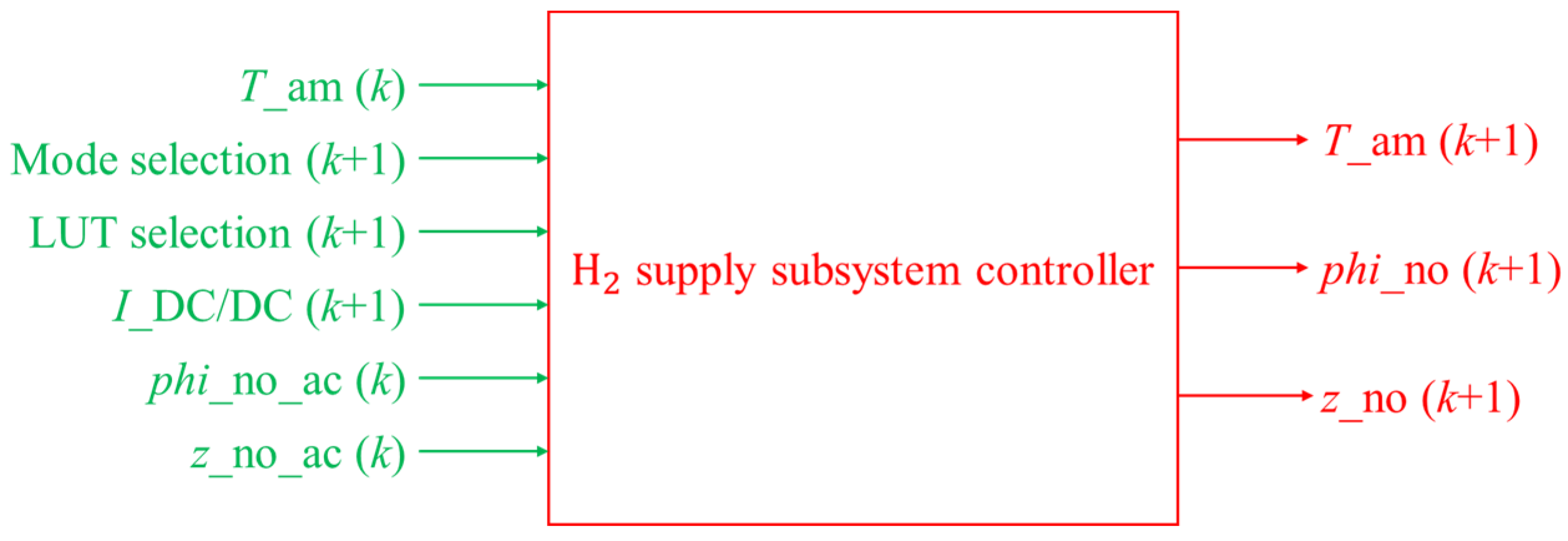
3.2.3. H₂ Supply Subsystem Controller

The H₂ supply subsystem controller shown in Figure 14 provides the ambient temperature and opening and damping of the variable damping nozzle to the CAN Out and H₂ supply subsystem module.

The ambient temperature and opening and damping of the variable damping nozzle to the CAN Out and H₂ supply subsystem module are expressed as:

$$T_{am}(k+1)=T_{am}\left(k\right)$$

(55)

$$ph{i}_{no}(k+1)=LUT\_ph{i}_{no}\left(I_{DC/DC}\right)+K_p\_ph{i}_{no}\times e\_ph{i}_{no}(k+1)$$

(56)

$$z_{no}(k+1)=LUT\_z_{no}\left(I_{DC/DC}\right)+K_p\_z_{no}\times e\_z_{no}(k+1)$$

(57)

where $LUT\_ph{i}_{no}\left(I_{DC/DC}\right),K_p\_ph{i}_{no},e\_ph{i}_{no}(k+1)=LUT\_ph{i}_{no}\left(I_{DC/DC}\right)-ph{i}_{no,ac}\left(k\right)$ are the feedforward table, proportional, and difference of the opening of the variable damping nozzle, respectively, $LUT\_z_{no}\left(I_{st}\right),K_p\_ph{i}_{th},e\_z_{no}(k+1)=LUT\_z_{no}\left(I_{st}\right)-z_{no,ac}\left(k\right)$ are the feedforward table, proportional, and difference of the damping of the variable damping nozzle, respectively.

3.2.4. Thermal Management Subsystem Controller

The thermal management subsystem controller shown in Figure 15 provides the ambient temperature, pump and fan speeds, and opening of the thermostat to the CAN Out and thermal management subsystem module.

The ambient temperature, pump and fan speeds, and opening of the thermostat to the CAN Out and thermal management subsystem module are expressed as:

$$T_{am}(k+1)=T_{am}\left(k\right)$$

(58)

$$n_{pu}(k+1)=LUT\_n_{pu}\left(I_{DC/DC}\right)+K_p\_n_{pu}\times e\_n_{pu}(k+1)$$

(59)

$$n_{fa}(k+1)=LUT\_n_{fa}\left(I_{DC/DC}\right)+K_p\_n_{fa}\times e\_n_{fa}(k+1)$$

(60)

$$ph{i}_{ther}(k+1)=LUT\_ph{i}_{ther}\left(I_{DC/DC}\right)+K_p\_ph{i}_{ther}\times e\_ph{i}_{ther}(k+1)$$

(61)

where $LUT\_n_{pu}\left(I_{DC/DC}\right),K_p\_n_{pu},e\_n_{pu}(k+1)=LUT\_n_{pu}\left(I_{DC/DC}\right)-n_{pu,ac}\left(k\right)$ are the feedforward table, proportional, and difference of the pump speed, respectively, $LUT\_n_{fa}\left(I_{DC/DC}\right),K_p\_n_{fa},e\_n_{fa}(k+1)=LUT\_n_{fa}\left(I_{DC/DC}\right)-n_{fa,ac}\left(k\right)$ are the feedforward table, proportional, and difference of the fan speed, respectively, $LUT\_ph{i}_{ther}\left(I_{DC/DC}\right),K_p\_ph{i}_{ther},e\_ph{i}_{ther}(k+1)=LUT\_ph{i}_{ther}\left(I_{DC/DC}\right)-ph{i}_{ther,ac}\left(k\right)$ is the feedforward table, proportional, and difference of the opening of the thermostat, respectively.

3.2.5. DC/DC Subsystem Controller

The DC/DC subsystem controller shown in Figure 16 provides the duty ratio and loading current of the DC/DC to the CAN Out and DC/DC module.

The duty ratio and loading current of the DC/DC to the CAN Out and DC/DC module are determined by the operating mode; if the operating mode selected is constant current, the duty ratio and loading current are expressed as:

$$r_{DC/DC}(k+1)=0.35$$

(62)

$$I_{DC/DC}(k+1)=70$$

(63)

While if the operating mode selected is constant power, the duty ratio and loading current are expressed as:

$$r_{DC/DC}(k+1)=LUT\left(\mathrm{m}\mathrm{i}\mathrm{n}\left\{I_d(k+1),\mathrm{m}\mathrm{i}\mathrm{n}\left[{\displaystyle \frac{4F\left(W_{ca,O_2,in}+W_{ca,O_2}\right)}{M_{O_2}\times nu{m}_{FC}}},{\displaystyle \frac{2F\left(W_{an,in}+W_{an}-\frac{d}{dt}(p_{an}\times V{o}_{an}/R/T_{an})\right)}{M_{H_2}\times nu{m}_{FC}}}\right]\right\}\right)$$

(64)

$$r_{DC/DC}(k+1)=\mathrm{m}\mathrm{i}\mathrm{n}\left\{I_d(k+1),\mathrm{m}\mathrm{i}\mathrm{n}\left[{\displaystyle \frac{4F\left(W_{ca,O_2,in}+W_{ca,O_2}\right)}{M_{O_2}\times nu{m}_{FC}}},{\displaystyle \frac{2F\left(W_{an,in}+W_{an}-\frac{d}{dt}(p_{an}\times V{o}_{an}/R/T_{an})\right)}{M_{H_2}\times nu{m}_{FC}}}\right]\right\}$$

(65)

where ${\mathrm{M}}_{{\mathrm{O}}_2}=32 \mathrm{g}/\mathrm{m}\mathrm{o}\mathrm{l}$ is the mole mass of O₂, ${\mathrm{M}}_{{\mathrm{H}}_2}=2.016 \mathrm{g}/\mathrm{m}\mathrm{o}\mathrm{l}$ is the mole mass of H₂, and $\mathrm{V}{\mathrm{o}}_{\mathrm{a}\mathrm{n}}=0.005 {\mathrm{m}}^3$ is the volume of the anode.

4. Results and Discussion

The output power of the PEMFC will decrease when the loading current is constant with the increase in operating time because of the voltage decrease caused by the component degradation of the PEMFC. Therefore, there are two operating modes of the PEMFC including the constant current (power reduction) and constant power (current rise) outputs. If the operating mode of constant current is selected, only the thermal management subsystem controller in the FCU needs to change because the heat generation caused by the voltage change has changed, while the other controllers do not need to be changed because the air and H₂ supply subsystem controllers are only dependent on the current. While if the operating mode of constant power is selected, the air and H₂ supply, thermal management subsystem, and DC/DC controllers need to change because the loading current of the PEMFC is constantly changing across the whole operating process when the output power is constant. Therefore, the operating mode of constant current is generally applied in the actual system, and the insufficient power is compensated for by the battery. The comparison of results for the operating mode of constant current with and without the proposed control framework is presented in detail. It was noted that only the results of the thermal management subsystem were different, while those of the other subsystems were the same.

4.1. Results Comparison of Stack

This section presents a comparison of the results of the RUL, SoH, loading current, voltage and power of stack with and without the proposed control framework.

The prediction results of the RUL with and without the proposed control framework are shown in Figure 17. It can be seen that the prediction results of the RUL could only be obtained by applying the proposed control framework, while there was no information of the RUL without the proposed control framework. The prediction of RUL started at 200 h and operated every 100 h. Moreover, the prediction results of the RUL decided the estimation duration of the SoH.

The estimation results of the SoH with and without the proposed control framework are shown in Figure 18. It can be seen that the estimation of the SoH could only be obtained by applying the proposed control framework, while there was no information of the SoH without the proposed control framework. The estimation of SoH started at 100 h, and its duration was 20 h in the period of 0–500 h, 10 h in the period of 500 h–700 h, and 5 h in the period above 700 h, respectively.

4.2. Results Comparison of Thermal Management Subsystem

This section presents the results comparison of the pump and fan speeds, opening of the thermostat, coolant flow rate, temperature of the pump outlet, and stack temperature with and without the proposed control framework.

The results of the pump speed with and without the proposed control framework are shown in Figure 19. The pump speed with/without the proposed control framework tended to increase because with the increase in the stack operating time, the stack performance degraded, which manifested in the gradual increase in the stack heat production pulling the same amount of current. Therefore, the heat dissipation needed to be increased to maintain the stack temperature in the appropriate range by increasing the pump speed. Specifically, the pump speed with the proposed control framework rose slowly from 500 r/min to 514 r/min at 0~712.86 h and fell slowly from 514 r/min to 507 r/min at 712.86~1000 h, while that without the proposed control framework rose from 500 r/min to 524 r/min at 0~1000 h. The control strategy without the proposed control framework simply increased the pump speed to realize the increase in heat dissipation.

The results of the fan speed with and without the proposed control framework are shown in Figure 20. The fan speed with/without the proposed control framework tended to increase because with the increase in the stack operating time, the stack performance degraded, which manifested in the gradual increase in the stack heat production pulling the same amount of current. Therefore, the heat dissipation needed to be increased to maintain the stack temperature in the appropriate range by increasing the pump speed. Specifically, the fan speed with the proposed control framework slowly increased from 1200 r/min to 1228 r/min at 0~500 h, slowly increased from 1331 r/min to 1336 r/min at 500~700 h, and slowly decreased from 1542 r/min to 1521 r/min at 700~1000 h, while that without the proposed control framework slowly increased from 1200 r/min to 1259 r/min at 0~1000 h.

The results of the opening of the thermostat with and without the proposed control framework are shown in Figure 21. The thermostat flow distribution coefficient with/without the control frame was 1 because the coolant is always running in large circulation when the stack is always in normal operation.

The results of the coolant flow rate of the pump outlet with and without the proposed control framework are shown in Figure 22. The coolant mass flow rate of the pump outlet with the proposed control framework rose slowly from 33.29 g/s to 34.24 g/s in 0~712.86 h, and decreased slowly from 34.24 g/s to 33.78 g/s in 712.86~1000 h, while that without the proposed control framework rose from 33.29 g/s to 34.94 g/s in 0~1000 h. It can be seen that the coolant mass flow rate of the pump outlet with the proposed control framework increased and then decreased, while that without the proposed control framework showed an increasing trend.

The results of the pump outlet temperature with and without the proposed control framework are shown in Figure 23. The coolant temperature of the pump outlet with/without the proposed control framework showed a decreasing trend. Specifically, the coolant temperature of the pump outlet with the proposed control framework slowly decreased from 325.16 K to 324.85 K in 0~500 h, decreased from 324.85 K to 324.74 K in 500~700 h, decreased from 324.74 K to 324.36 K in 700~832 h, and increased from 324.36 K to 324.38 K in 832~1000 h, while that without the proposed control framework decreased from 325.16 K to 324.90 K in 0~1000 h.

The results of the stack temperature with and without the proposed control framework are shown in Figure 24. The stack temperature with/without the proposed control framework was very close because the power level of the stack was low, so the heat production was not obvious enough, but the change trend of the stack temperature could reflect the control effect. If the stack temperature increases, the control strategy cannot pull the stack temperature back to the desired temperature, which indicates that the control strategy is unable to control the stack temperature for a longer period of operation or in the case of a high output power of the stack. On the contrary, if the stack temperature shows a rising and then falling trend, the control strategy can bring the stack temperature back to the desired temperature, which indicates that the strategy can still control the stack temperature for a longer period of operation or in the case of a high output power of the stack. The stack temperature with the proposed control framework showed a trend of increase and then decrease, while that without the proposed control framework showed a constant increasing trend. Specifically, the stack temperature with the proposed control framework rose slowly from 327.15 K to 327.16 K in 0~530 h, was basically maintained at 327.16 K in 530~711 h, decreased slowly from 327.16 K to 327.15 K in 711~1000 h, while that without proposed control framework increased from 327.15 K to 327.15 K in 0~1000 h, and then increased from 327.15 K to 327.15 K in 711~1000 h and 327.15 K to 327.17 K in 0~1000 h.

5. Conclusions

This study designed a control framework to solve the control problems caused by PEMFC performance degradation. The detailed conclusions are as follows:

(a)

This work described the modeling principles of the plant module including models of the anode channel, cathode channel, coolant channel, voltage calculation, and thermal management subsystems in detail.

(b)

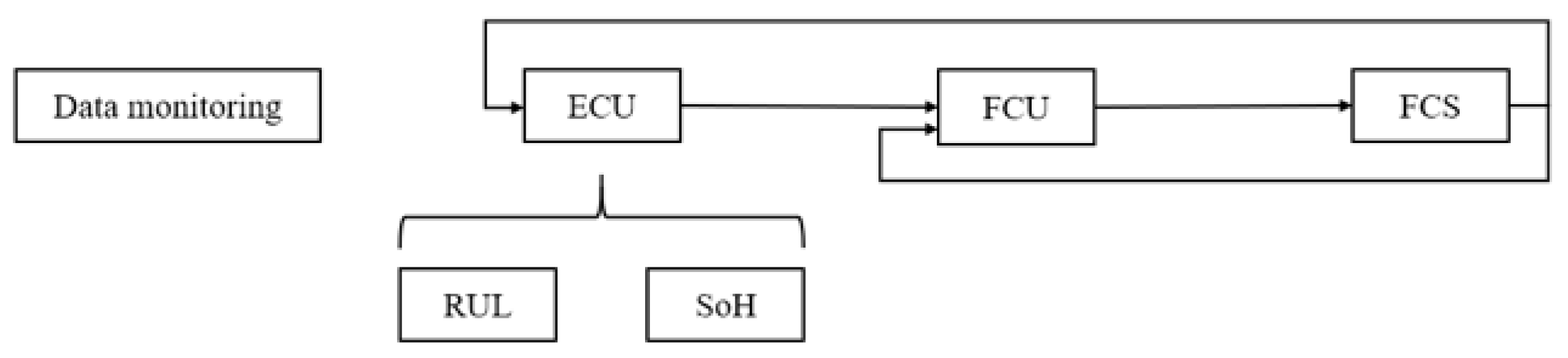
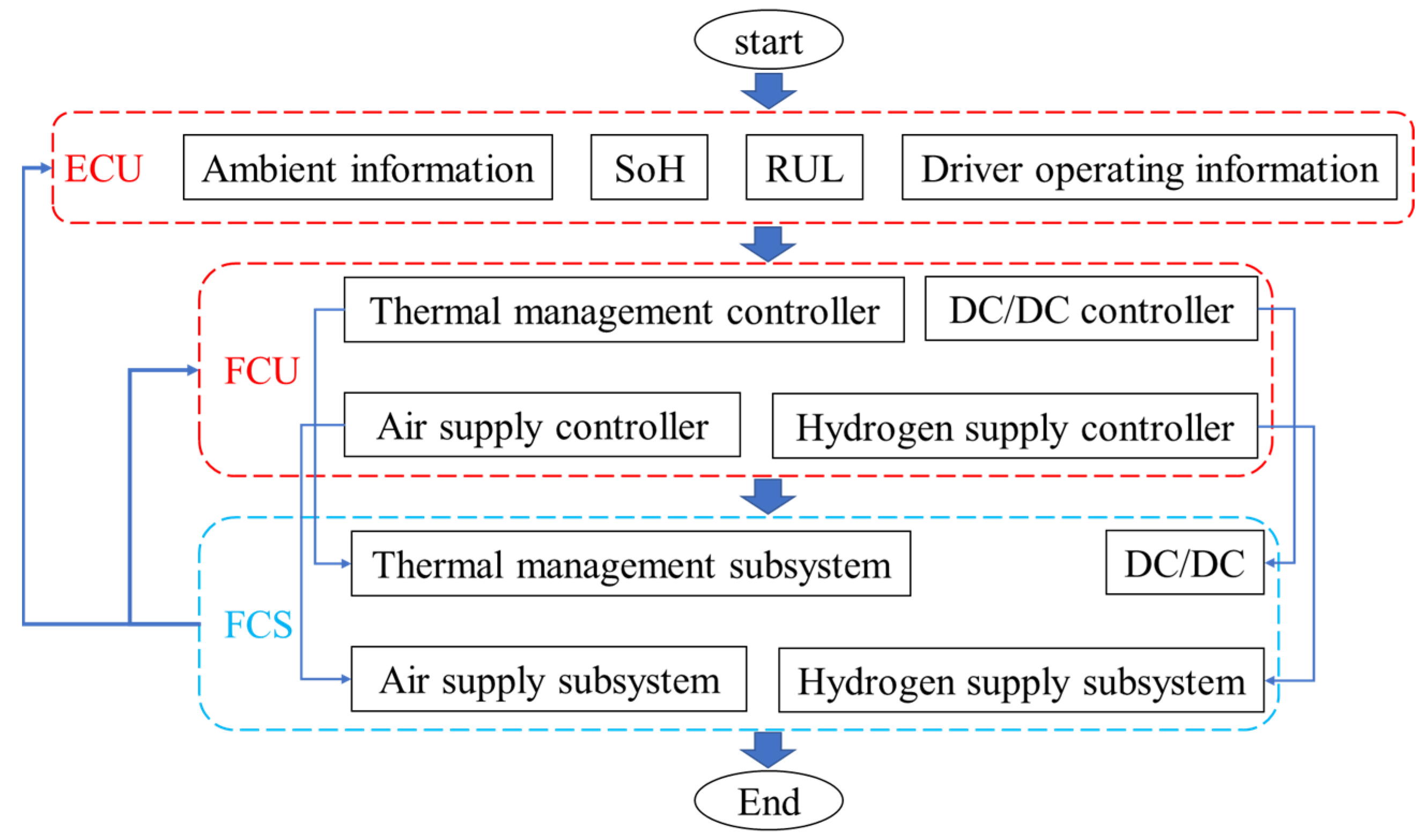
This work designed a novel control framework including ECU, RUL, SoH, and FCU modules. This control framework introduces the results of the SoH estimation and RUL prediction to the ECU and FCU. The desired power of the stack was obtained, which was used as the real-time desired power of the PEMFC system by synthesizing the RUL, SoH, and ECU information of the stack.

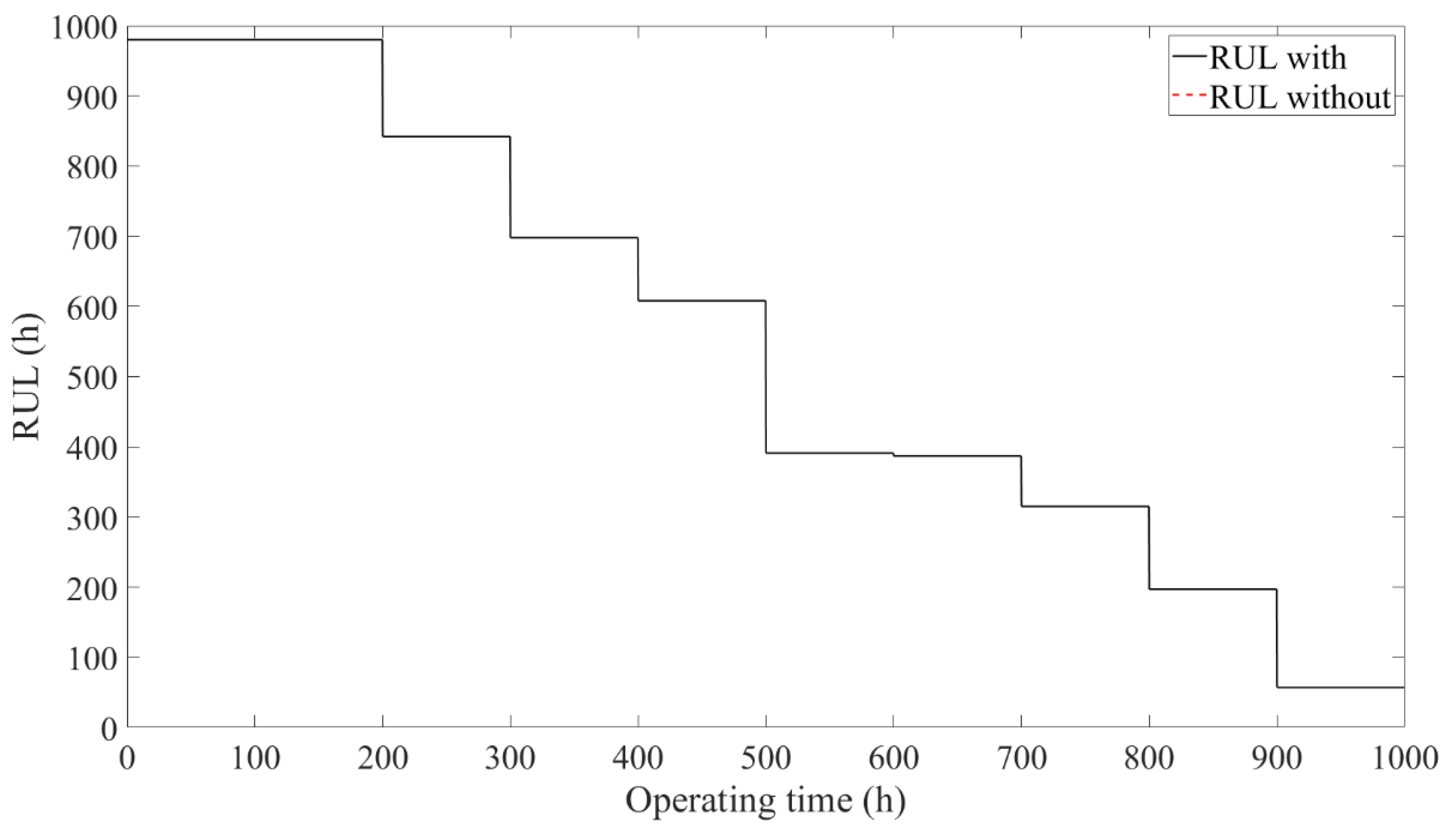
(c)

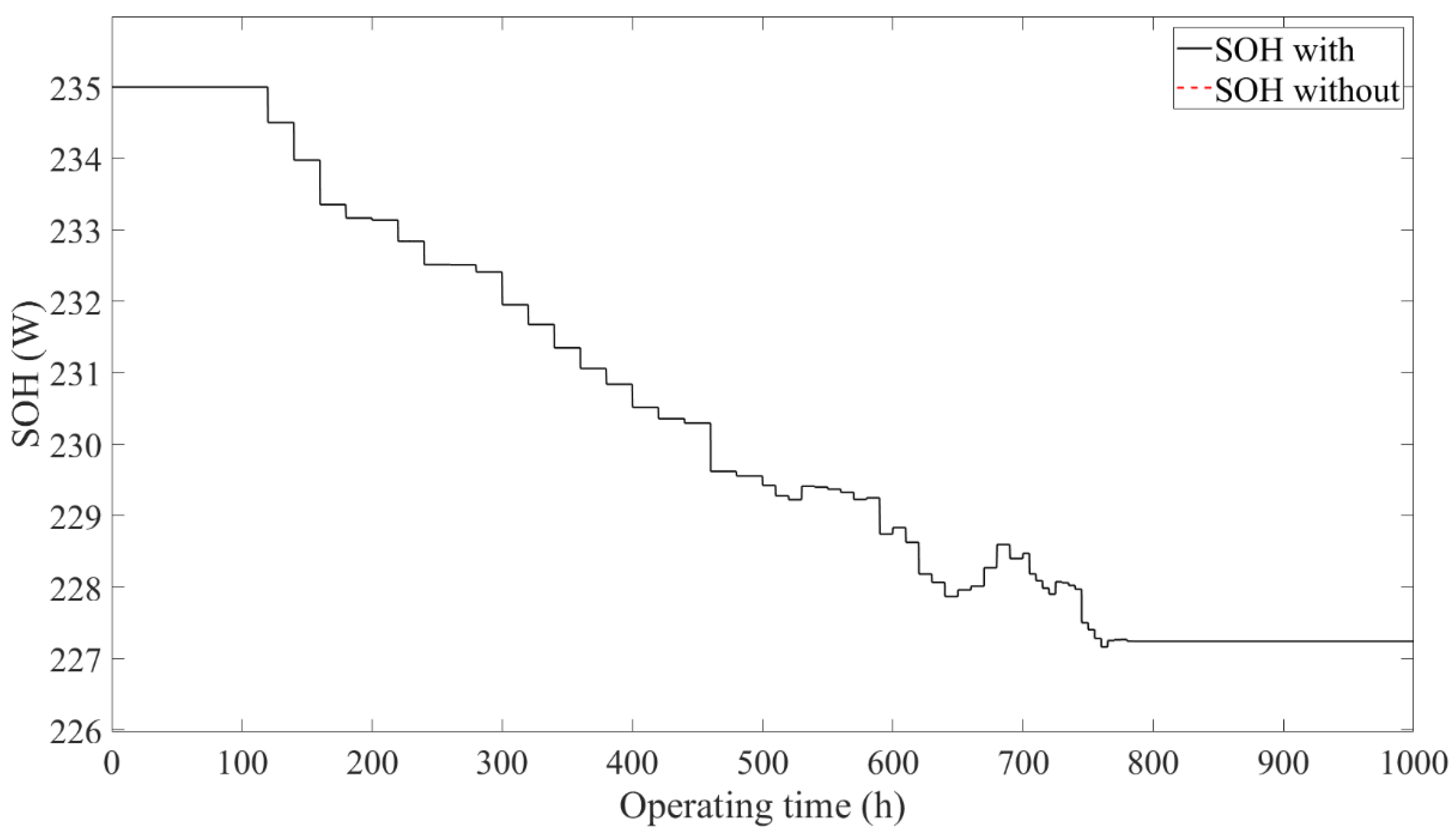
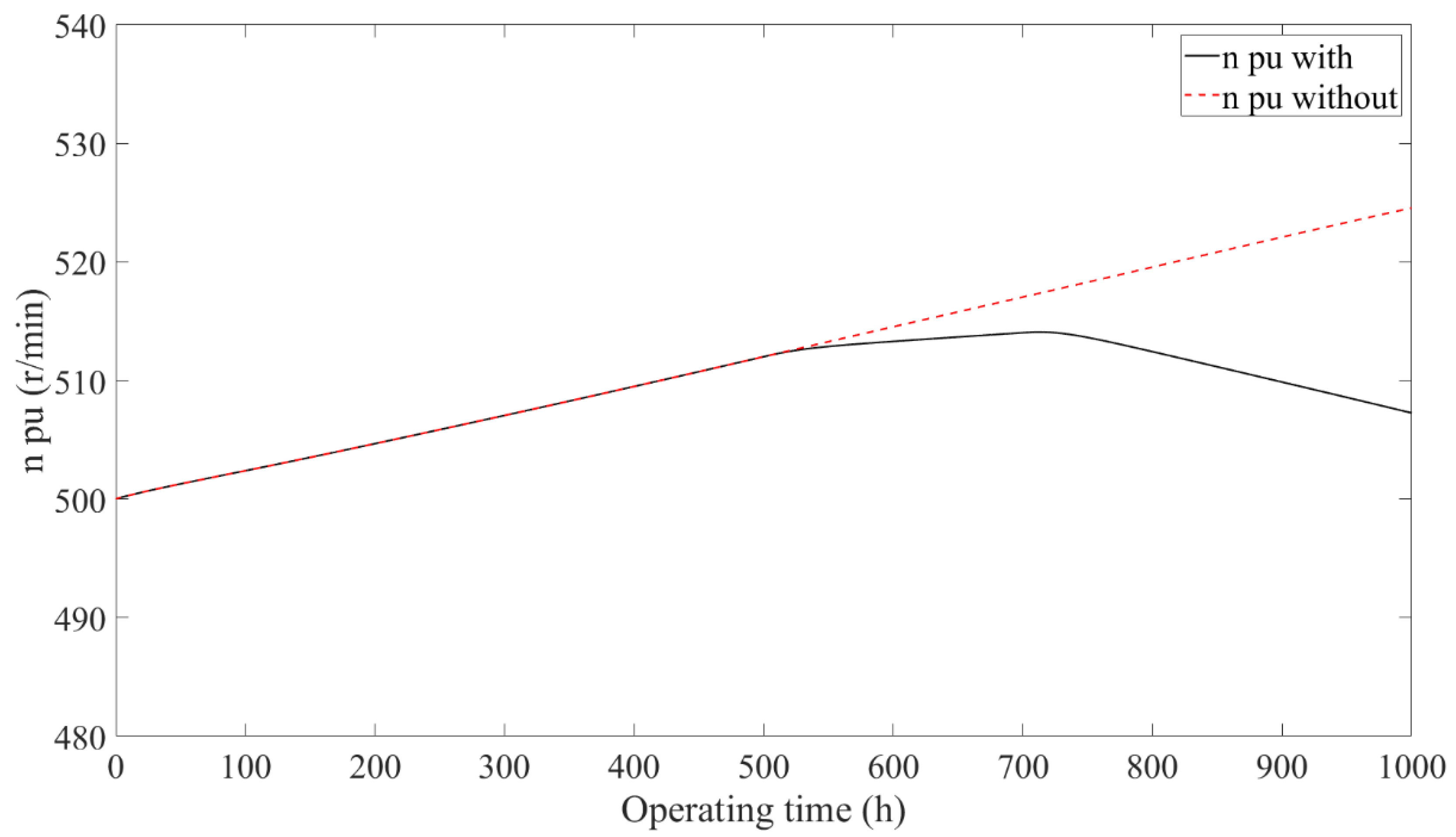
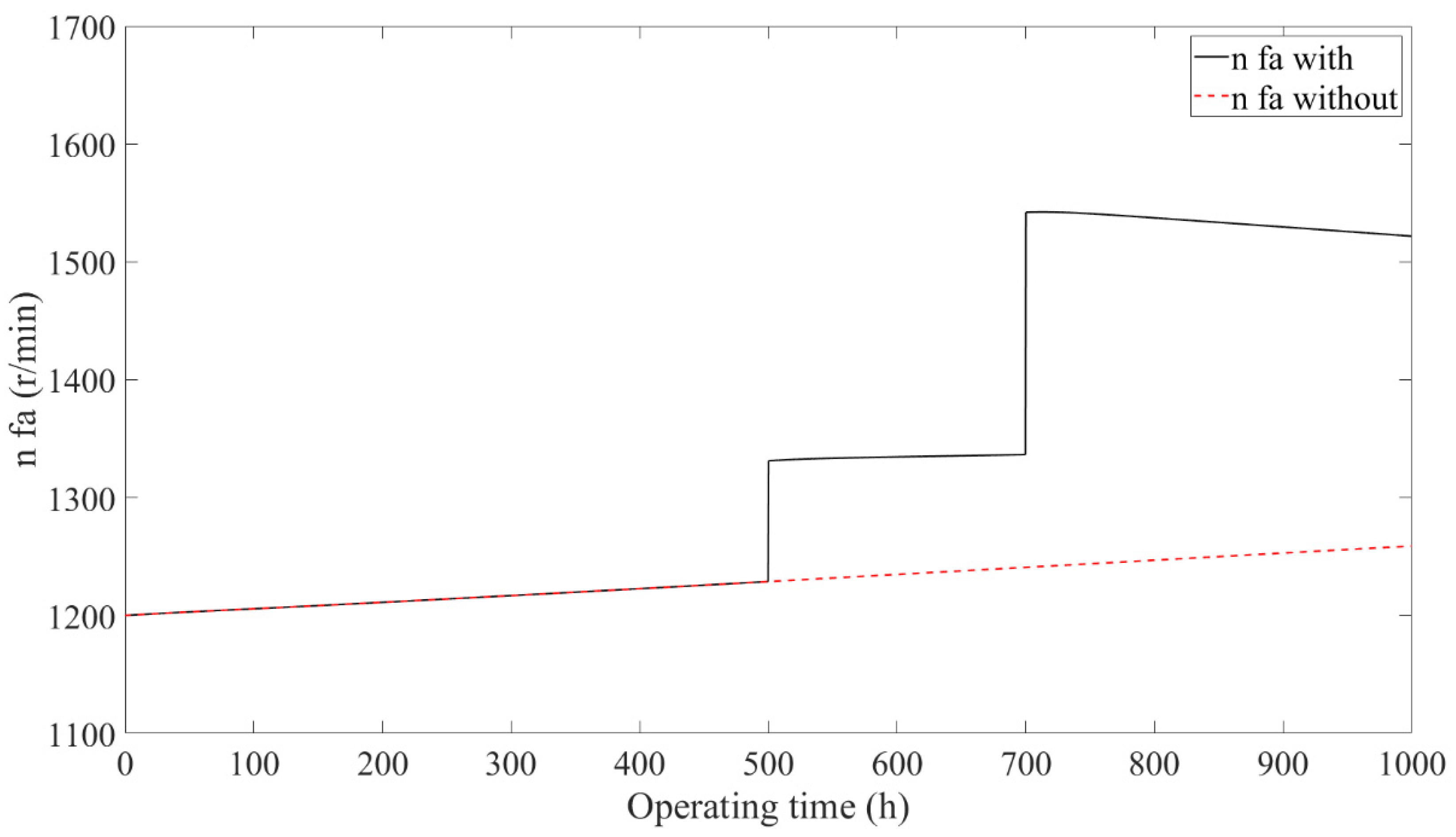
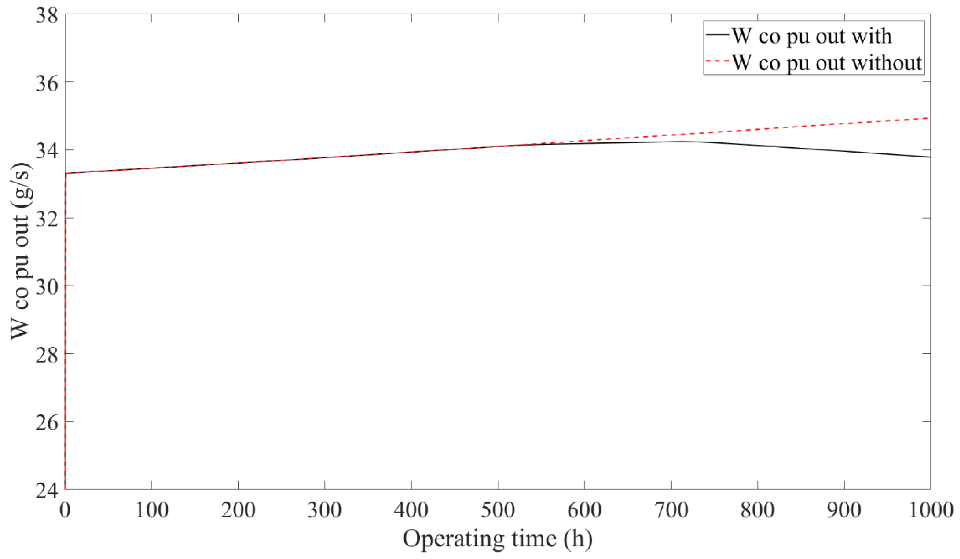
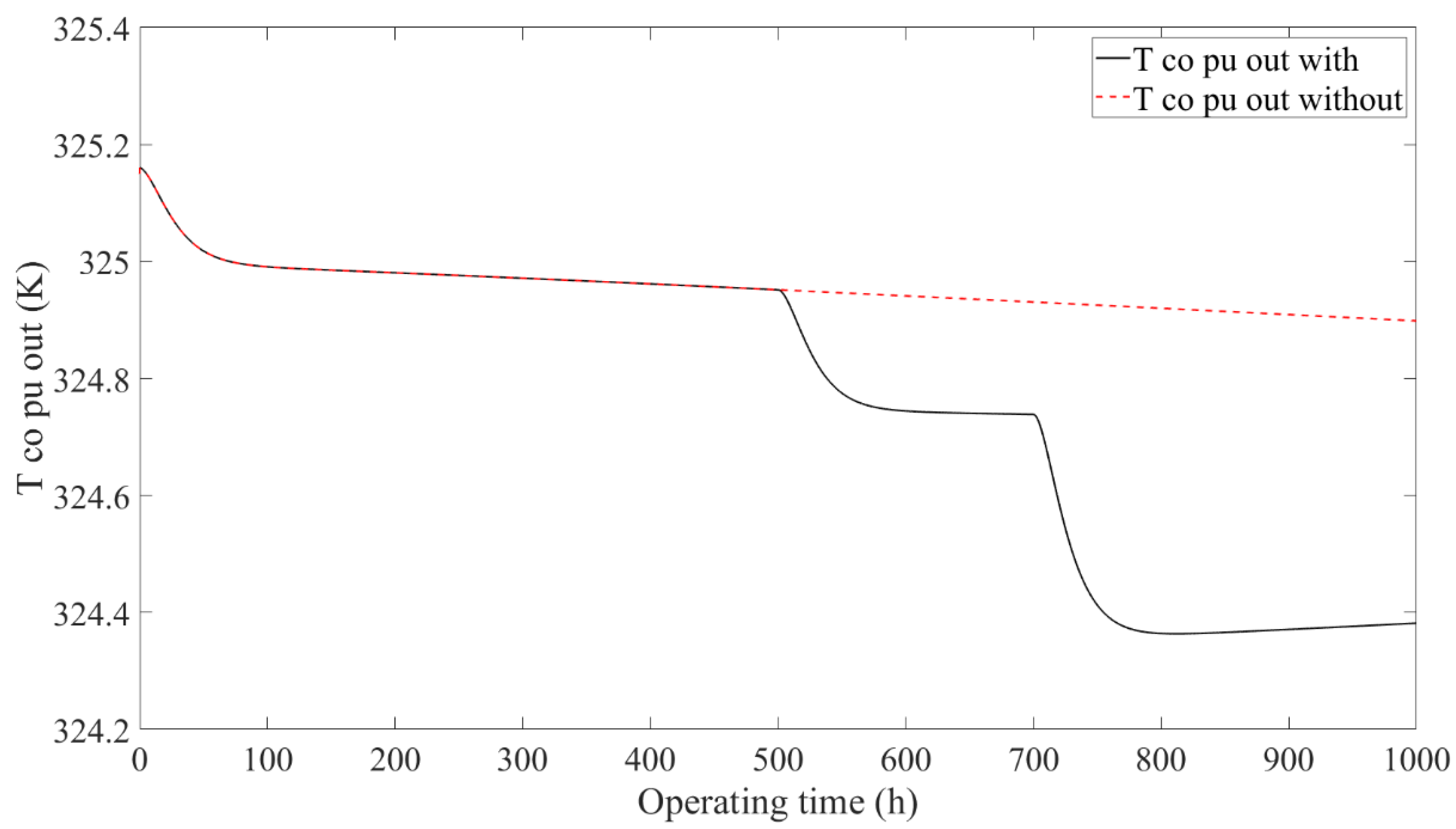
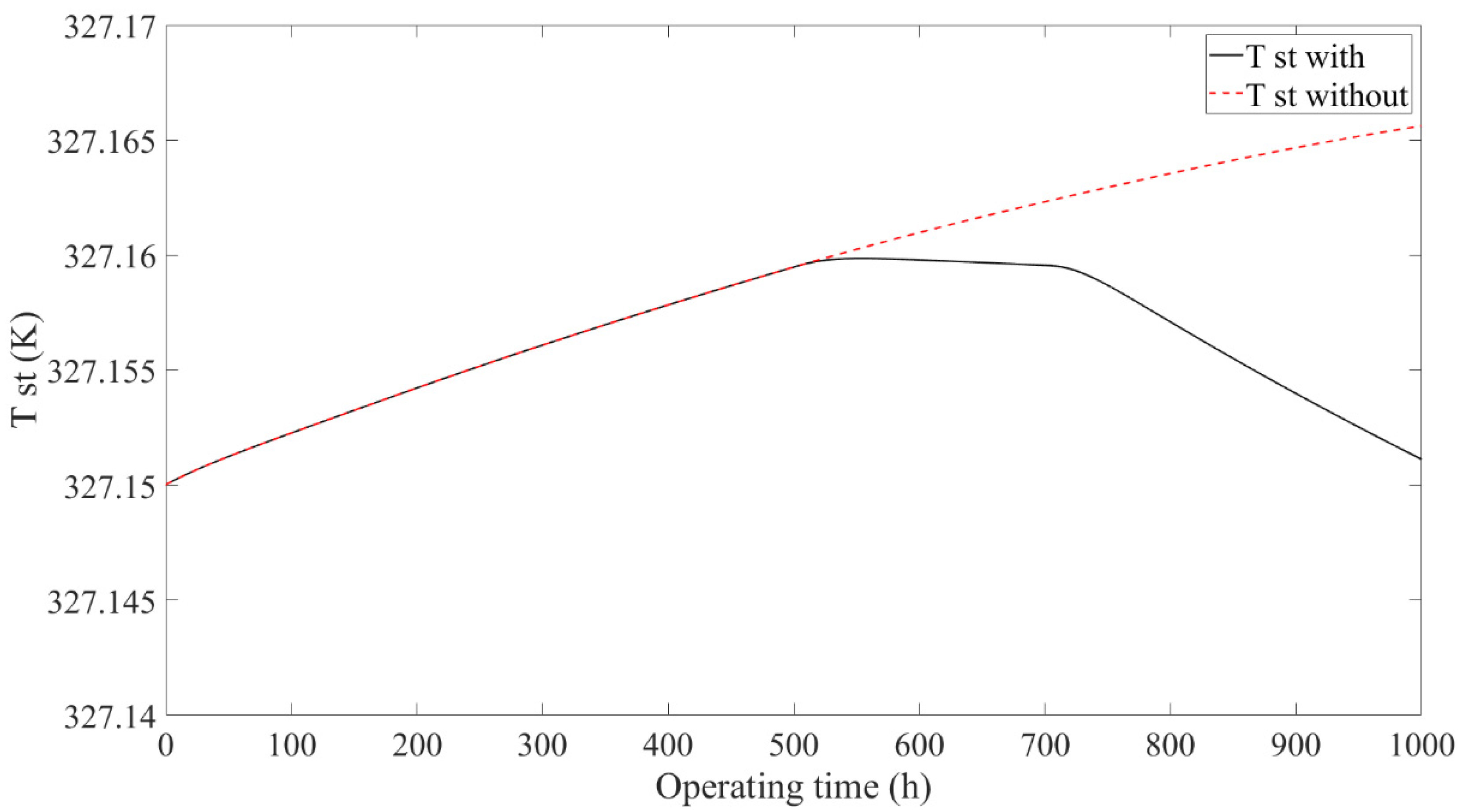
The two operation modes after performance degradation of the stack, including constant current reducing power and constant power rising current, were analyzed. Furthermore, the output of the subsystem controllers and actuators were analyzed in detail under the operation mode of constant current reducing power. The results showed that when the PEMFC system was operated under the operation mode of constant current reducing power, the results of the air and hydrogen supply and DC/DC subsystems with/without the designed control framework were the same, while the thermal management subsystems showed different results. When the PEMFC system disused the designed control framework, the stack temperature showed a monotonically increasing trend, which indicates that the stack temperature tended to get out of control with the increase in the operation time. However, when the PEMFC system used the designed control framework, the stack temperature showed an increasing and then decreasing trend, which indicates that the stack temperature was still controllable.

(d)

The aim of this work was to verify the effectiveness of the proposed framework for PEMFC operation temperature control. This work was not experimentally verified due to the limitation of the experimental conditions and cost, and the control algorithms of each subsystem used PID control, which has not involved complex algorithms yet.

References

- Onanena, R.; Oukhellou, L.; Candusso, D.; Same, A.; Hissel, D.; Aknin, P. Estimation of fuel cell operating time for predictive maintenance strategies. Int. J. Hydrogen Energy 2010, 35, 8022–8029. [Google Scholar] [CrossRef]
- Zenith, F.; Tjonnas, J.; Halvorsen, I.J. Control structure of a micro combined heat and power fuel-cell system for lifetime maximisation. In Proceedings of the 2014 IEEE Vehicle Power and Propulsion Conference (Vppc), Coimbra, Portugal, 27–30 October 2014; pp. 1–6. [Google Scholar]
- Fletcher, T.; Thring, R.; Watkinson, M. An Energy Management Strategy to concurrently optimise fuel consumption & PEM fuel cell lifetime in a hybrid vehicle. Int. J. Hydrogen Energy 2016, 41, 21503–21515. [Google Scholar]
- Jouin, M.; Gouriveau, R.; Hissel, D.; Pera, M.C.; Zerhouni, N. Combined predictions for prognostics and predictive control of transportation PEMFC. IFAC-PapersOnLine 2016, 49, 244–249. [Google Scholar] [CrossRef]
- Fu, X.; Pei, P.; Ren, P.; Zhu, Z.; Wang, H.; Song, X.; Wang, Z. On-board and in-situ identification of cell-individual hydrogen crossover in fuel cell stacks based on electrochemical dynamics during shutdown. Chem. Eng. J. 2025, 506, 159952. [Google Scholar] [CrossRef]
- Du, Y.; Li, Y.; Ren, P.; Zhang, L.; Wang, D.; Xu, X. Oxygen transfer at mesoscale catalyst layer in proton exchange membrane fuel cell: Mechanism, model and resistance characterization. Chem. Eng. J. 2024, 494, 153021. [Google Scholar] [CrossRef]
- Tjonnas, J.; Zenith, F.; Halvorsen, I.J.; Klages, M.; Scholta, J. Control of Reversible Degradation Mechanisms in Fuel Cells: Mitigation of CO contamination. IFAC-PapersOnLine 2016, 49, 302–307. [Google Scholar] [CrossRef]
- Polverino, P.; Pianese, C. Control algorithm design for degradation mitigation and lifetime improvement of Polymer Electrolyte Membrane Fuel Cells. Energy Procedia 2017, 142, 1706–1713. [Google Scholar] [CrossRef]
- Yue, M.L.; Jemei, S.; Gouriveau, R.; Zerhouni, N. Developing a Health-Conscious Energy Management Strategy based on Prognostics for a Battery/Fuel cell Hybrid Electric Vehicle. In Proceedings of the 2018 IEEE Vehicle Power and Propulsion Conference (Vppc), Chicago, IL, USA, 27–30 August 2018; pp. 1–6. [Google Scholar]
- Yue, M.; Jemei, S.; Zerhouni, N. Health-Conscious Energy Management for Fuel Cell Hybrid Electric Vehicles Based on Prognostics-Enabled Decision-Making. IEEE Trans. Veh. Technol. 2019, 68, 11483–11491. [Google Scholar] [CrossRef]
- Li, H.; Ravey, A.; N’Diaye, A.; Djerdir, A. Online adaptive equivalent consumption minimization strategy for fuel cell hybrid electric vehicle considering power sources degradation. Energy Convers. Manag. 2019, 192, 133–149. [Google Scholar] [CrossRef]
- Wu, X.; Xu, L.; Wang, J.; Yang, D.; Li, F.; Li, X. A prognostic-based dynamic optimization strategy for a degraded solid oxide fuel cell. Sustain. Energy Technol. Assess. 2020, 39, 100682. [Google Scholar] [CrossRef]
- Lin, X.; Li, X.; Shen, Y.; Li, H. Charge depleting range dynamic strategy with power feedback considering fuel-cell degradation. Appl. Math. Model. 2020, 80, 345–365. [Google Scholar] [CrossRef]
- Bressel, M.; Hilairet, M.; Hissel, D.; Ould Bouamama, B. Model-based aging tolerant control with power loss prediction of Proton Exchange Membrane Fuel Cell. Int. J. Hydrogen Energy 2020, 45, 11242–11254. [Google Scholar] [CrossRef]
- Hahn, S.; Braun, J.; Kemmer, H.; Reuss, H.-C. Optimization of the efficiency and degradation rate of an automotive fuel cell system. Int. J. Hydrogen Energy 2021, 46, 29459–29477. [Google Scholar] [CrossRef]
- Fan, L.; Zhou, S.; Wen, C.; Gao, J. Prediction of the Remaining Useful Life of the Proton Exchange Membrane Fuel Cell with an Integrated Health Index; SAE Technical Paper Series; SAE International: Warrendale, PA, USA, 2023. [Google Scholar]
- Fan, L.; Zhou, S.; Zhao, P.; Gao, J. A Novel Hybrid Method Based on the Sliding Window Method for the Estimation of the State of Health of the Proton Exchange Membrane Fuel Cell; SAE Technical Paper Series; SAE International: Warrendale, PA, USA, 2023. [Google Scholar]
Disclaimer/Publisher’s Note: The statements, opinions and data contained in all publications are solely those of the individual author(s) and contributor(s) and not of MDPI and/or the editor(s). MDPI and/or the editor(s) disclaim responsibility for any injury to people or property resulting from any ideas, methods, instructions or products referred to in the content. |
© 2025 by the authors. Licensee MDPI, Basel, Switzerland. This article is an open access article distributed under the terms and conditions of the Creative Commons Attribution (CC BY) license (https://creativecommons.org/licenses/by/4.0/).
Share and Cite
Fan, L.; Gao, J.; Shen, W.; Su, H.; Zhou, S.; Hou, Y. A Control Framework for the Proton Exchange Membrane Fuel Cell System Integrated the Degradation Information. Energies 2025, 18, 2438. https://doi.org/10.3390/en18102438
Fan L, Gao J, Shen W, Su H, Zhou S, Hou Y. A Control Framework for the Proton Exchange Membrane Fuel Cell System Integrated the Degradation Information. Energies. 2025; 18(10):2438. https://doi.org/10.3390/en18102438
Chicago/Turabian StyleFan, Lei, Jianhua Gao, Wei Shen, Hongtao Su, Su Zhou, and Yiwei Hou. 2025. "A Control Framework for the Proton Exchange Membrane Fuel Cell System Integrated the Degradation Information" Energies 18, no. 10: 2438. https://doi.org/10.3390/en18102438
APA StyleFan, L., Gao, J., Shen, W., Su, H., Zhou, S., & Hou, Y. (2025). A Control Framework for the Proton Exchange Membrane Fuel Cell System Integrated the Degradation Information. Energies, 18(10), 2438. https://doi.org/10.3390/en18102438