A Deep Learning Method for Photovoltaic Power Generation Forecasting Based on a Time-Series Dense Encoder

Abstract

Deep learning has become a widely used approach in photovoltaic (PV) power generation forecasting due to its strong self-learning and parameter optimization capabilities. In this study, we apply a deep learning algorithm, known as the time-series dense encoder (TiDE), which is an MLP-based encoder–decoder model, to forecast PV power generation. TiDE compresses historical time series and covariates into latent representations via residual connections and reconstructs future values through a temporal decoder, capturing both long- and short-term dependencies. We trained the model using data from 2020 to 2022 from Australia’s Desert Knowledge Australia Solar Centre (DKASC), with 2023 data used for testing. Forecast accuracy was evaluated using the $R^2$ coefficient of determination, mean absolute error (MAE), and root mean square error (RMSE). In the 5 min ahead forecasting test, TiDE demonstrated high short-term accuracy with an $R^2$ of 0.952, MAE of 0.150, and RMSE of 0.349, though performance declines for longer horizons, such as the 1 h ahead forecast, compared to other algorithms. For one-day-ahead forecasts, it achieved an $R^2$ of 0.712, an MAE of 0.507, and an RMSE of 0.856, effectively capturing medium-term weather trends but showing limited responsiveness to sudden weather changes. Further analysis indicated improved performance in cloudy and rainy weather, and seasonal analysis reveals higher accuracy in spring and autumn, with reduced accuracy in summer and winter due to extreme conditions. Additionally, we explore the TiDE model’s sensitivity to input environmental variables, algorithmic versatility, and the implications of forecasting errors on PV grid integration. These findings highlight TiDE’s superior forecasting accuracy and robust adaptability across weather conditions, while also revealing its limitations under abrupt changes.

1. Introduction

Photovoltaic (PV) energy is regarded as one of the most promising opportunities in the renewable energy industry due to its clean and abundant nature [1]. In recent years, with the improvement of technology and capital investment, PV electric generation has received more attention worldwide [2]. The dramatic drop in solar PV costs has fueled a rapid expansion in global capacity, with solar expected to account for 80% of renewable energy growth by 2030, surpassing wind and hydropower as the largest renewable source [3]. However, due to the influence of factors such as environmental changes, PV power output has large fluctuations [4,5]. Therefore, accurately predicting PV power generation based on environmental variables is an important task, as it can optimize power dispatching, ensure grid stability, and improve energy utilization efficiency and economic benefits.

PV power forecasting is an important topic, but in actual systems, it needs to take into account many issues, such as the time stamp, weather data collection, input correlation analysis, data pre- and post-processing, etc. [6,7,8]. In past studies, physical and statistical methods were mainly used to address this type of problem [9]. Based on the fundamental physical interactions between solar panel cells and the environment, physical models predict the output of PV systems by the design of the mathematical formula model, and their accuracy is highly sensitive to input data quality via dynamic weather conditions [10,11]. Statistical methods analyze the relationship between meteorological factors and PV power generation, with accuracy dependent on the forecast horizon and input data quality [12]. Widely used techniques include regression and autoregression [13,14]; furthermore, autoregressive moving average (ARMA) [15], autoregressive-integrated moving average (ARIMA) [16], and exponential smoothing [17] have also been applied to PV power forecasting. Their prediction performance is good for linear data, but they face challenges with the nonlinear relationships between complex variables.

With the development of computer technology, machine learning (ML) has emerged as an important approach for PV power forecasting; techniques such as support vector regression (SVR) [18,19,20], decision tree (DT) [21], and extreme learning machine (ELM) [22] have been applied. These conventional ML methods are promising approaches, but they struggle with large datasets and are overly dependent on the complexity of the data and feature extraction. To enhance the ability to process big data, neural network (NN) algorithms were introduced to deal with the problem of PV power forecasting, increasing the accuracy of prediction [23,24,25,26]. Recurrent neural networks (RNNs) and long short-term memory (LSTM) methods in deep learning (DL) are also applicable to PV prediction problems, as they can fully extract hidden information in time series and capture the correlation between historical data and future forecasts [27,28,29].

With the widespread availability of high-performance computing servers, particularly GPU-based computing devices and algorithms, the application of advanced models in PV power forecasting is no longer limited to ML approaches of a simple structure. An improved sparrow search algorithm (ISSA)-optimized LSTM (ISSA-LSTM) model [30] and temporal convolutional networks (TCNs) have been employed to achieve high-accuracy, hour-level PV power forecasting under various weather conditions and seasons [31]. A hybrid model combining one-dimensional convolutional neural networks (1D-CNNs) and Transformer architecture achieves multi-step forecasting from 5 min to hour-level resolutions through multi-timescale fusion [32]. Artificial neural networks (ANNs), combined with gray wolf optimization (GWO) and genetic algorithms (GAs), have been utilized to optimize model structures and improve short-term forecasting accuracy [33]. The Fourier graph neural network (FourierGNN) captures spatiotemporal dependencies in PV data by constructing a hypervariable graph and applying Fourier transforms [34]. Most of these studies focus on short-term forecasting at minute- and hour-level resolutions. This is because, for short-interval data, e.g., 5 min intervals, the length of the daily time series becomes too long, posing challenges for memory-based DL models. Additionally, training neural network models on such long sequences often results in GPU memory overload, making high-performance hardware a necessary requirement for these tasks.

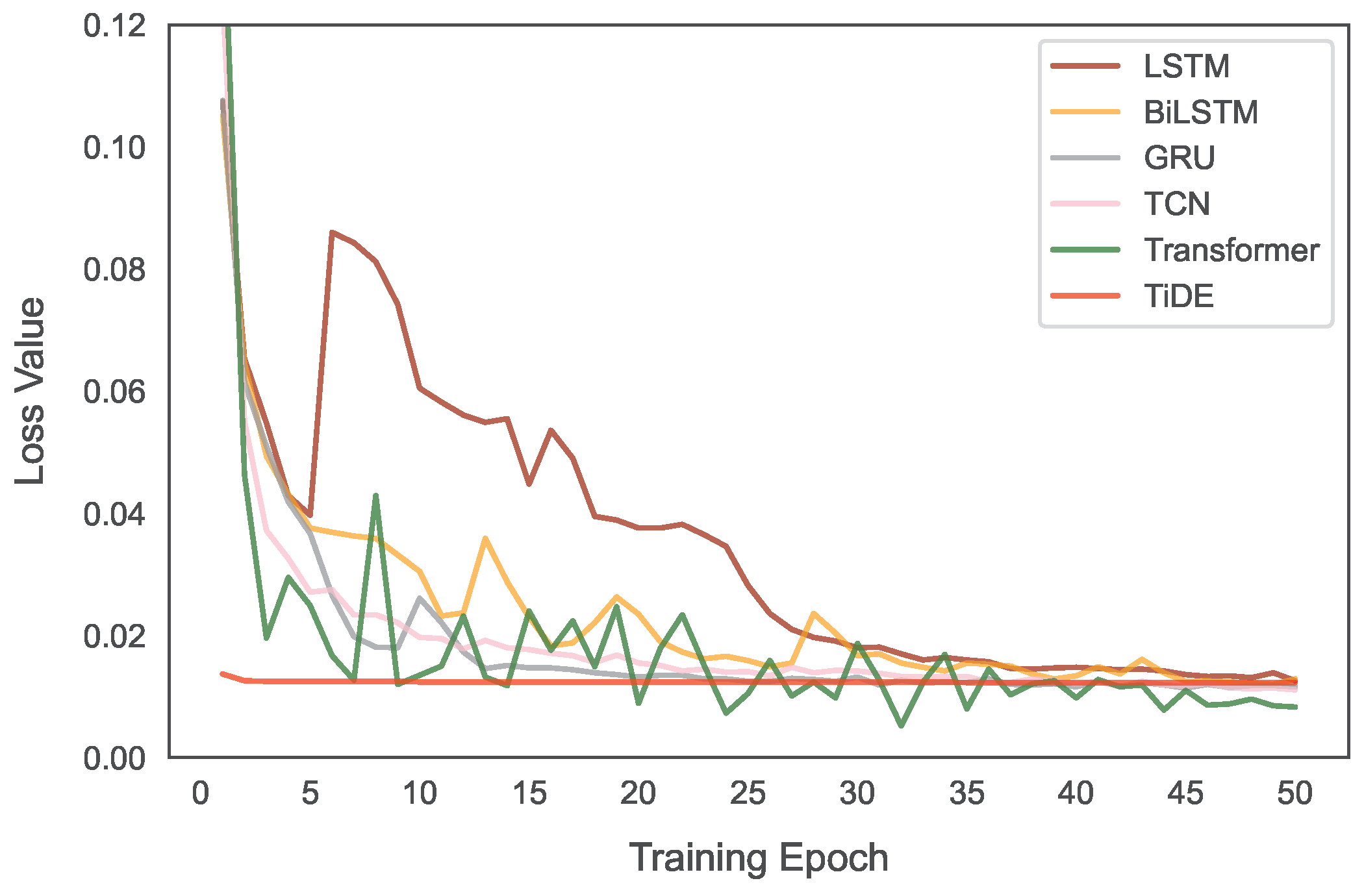
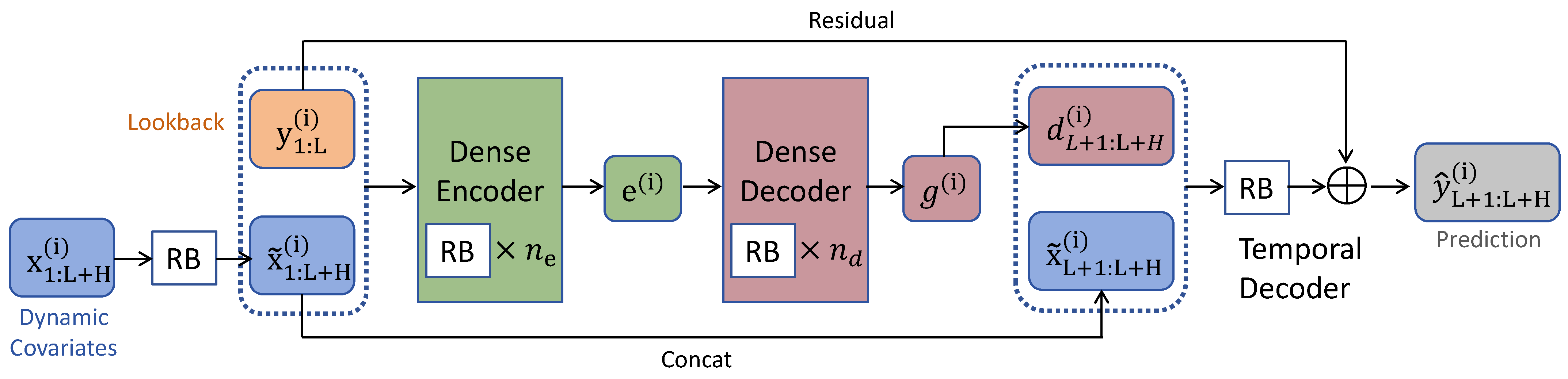
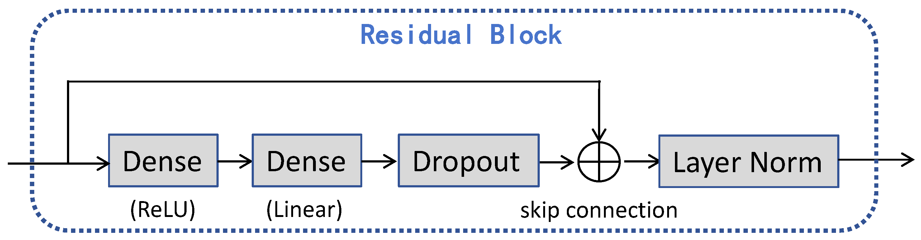
The time-series dense encoder (TiDE) is a multi-layer perceptron (MLP)-based encoder–decoder architecture, which combines the efficiency of linear models with the expressive power of nonlinear models [35]. Through feature projection and dense residual blocks, TiDE effectively integrates dynamic covariates and static covariates. In the architecture of TiDE, global linear residual connections preserve linear trend information, enhancing the model’s robustness in scenarios with complex dependencies. With its linear computational complexity, TiDE enables faster training and inference compared to Transformer-based models, making it particularly suitable for medium- to long-term time series forecasting. For PV power forecasting, TiDE can demonstrate strong capabilities in modeling nonlinear relationships between generation output and dynamic environmental variables such as solar irradiance, temperature, and seasonal effects. Its residual structure separates linear trends, like seasonal cycles, from nonlinear fluctuations, like abrupt weather changes, thereby improving prediction accuracy. Dimensionality reduction on large-scale covariates also reduces noise introduced by high-dimensional meteorological data, ensuring model stability under complex environmental conditions. For short-term forecasting, TiDE’s computational efficiency supports high-frequency data updates, meeting the real-time scheduling demands of PV power systems. These features make TiDE a highly efficient and reliable solution for PV power forecasting.

In this paper, we study the application of TiDE in forecasting short-term (5 min and 1 h ahead) and medium-term (1-day-ahead) PV power outputs using environmental variables. A dataset spanning three years is used for training, with the following one-year data serving as the test set to evaluate TiDE’s forecasting accuracy. Additionally, we analyze forecasting performance under various weather conditions, i.e., sunny, cloudy, and rainy, to assess TiDE’s power to capture both weather trends and abrupt changes in one-day-ahead forecasts. We also evaluate its performance across different seasons of climatic conditions to test the model’s adaptability and accuracy in diverse environments. Furthermore, we examine TiDE’s responsiveness to environmental input variables, its flexibility in handling different conditions, and the impact of forecasting errors on the integration of PV power into the grid. The results emphasize TiDE’s exceptional forecasting accuracy and strong adaptability to varying weather patterns, while also identifying its challenges in dealing with sudden changes. The remaining content of this paper is structured in the following manner. In Section 2, we provide the details of data preprocessing and the specific architecture of the TiDE algorithm used in the study. Section 3 shows the results of 5 min, 1 h, and 1-day-ahead PV power forecasting of TiDE. And in this part, we also analyze the one-day-ahead forecasting values of different weather types and seasons. Section 4 presents a discussion of TiDE’s sensitivity to input environmental variables, algorithmic versatility, and the implications of forecasting errors on PV grid integration. Section 5 presents the summary of this work.

2. Materials and Methods

2.1. Data Preprocessing

In this study, we use data from the Desert Knowledge Australia Solar Centre (DKASC) in Alice Springs, Australia. The PV power plant selected for analysis is the Calyxo system, an amorphous silicon installation with a 5.4 kW capacity, which has been operational since 2010 (in Section 4.2, a Kaneka system—an amorphous silicon installation with a capacity of 6.0 kW built in 2008—will be presented to briefly illustrate the breadth of algorithm applications). The dataset contains active PV generation and real-time environmental variables, such as temperature in Celsius, relative humidity, daily rainfall, etc., which are listed in

Table 1. Statistical data on the environmental variables.

Variable	Correlation Coefficient	Mean	Standard Deviation	Unit
Temperature (Celsius)	0.28	24.36	9.86	°C
Relative Humidity	−0.38	29.44	20.37	%
Global Horizontal Radiation	0.97	520.45	363.27	W/m2
Diffuse Horizontal Radiation	0.25	109.94	109.48	W/m2
Wind Direction	0.03	30.01	15.33	°
Daily Rainfall	−0.08	0.49	2.56	mm

. The data were recorded at five-minute intervals, and we restricted the dataset to the period between 07:00 and 19:00 each day to enhance the reliability and stability of the forecasts since PV systems generate negligible power at night. For our deep learning-based PV power prediction study, we used data from 2020 to 2022 as the training set and data from 2023 as the test set.

To ensure data quality, we applied preprocessing techniques to handle missing values of PV power generation. Specifically, data interruptions exceeding one day were removed in full-day units with related environmental variables, while interruptions shorter than one day were interpolated to maintain consistency in the dataset for deep learning algorithms. Additionally, when the number of missing data points within a day exceeded 10, the data for that entire day were excluded. Among them, missing values in the PV power generation data accounted for 1.84% of the total data, and 2.21% of the data were deleted during preprocessing. This proportion was less than 3%, which did not affect the learning and processing of data by the DL algorithm. For the environmental variable data, only a small portion (less than 0.1%) is not recorded, which can be filled using interpolation to ensure data completeness.

Furthermore, for environmental variables like temperature in Celsius and relative humidity, some of them exhibit strong correlations with PV output, while others have minimal impact. To improve the ability of the deep learning model to capture the intrinsic relationships among data features, we compute the correlation between each environmental variable and PV power output. As shown in Table 1, only environmental variables with an absolute correlation value greater than 0.25 are retained for analysis. This not only helps improve the learning efficiency of DL algorithms, but also greatly reduces the resources and time consumed by computing. To more accurately select the input environmental variables, we will discuss the use of mutual information to screen features and the impact of using other environmental factors as input on the output in Section 4.2.

In the process of deep learning, normalization ensures consistency in the magnitude of each element in the original dataset, facilitating improved feature learning efficiency, enhanced prediction accuracy, and increased training speed for deep learning algorithms. In our study, this normalization process is defined as follows:

$$p_n={\displaystyle \frac{p-p_{\min }}{P_{\max }-P_{\min }}},$$

(1)

where each input element is normalized by subtracting its minimum value $P_{\min }$ and scaling it relative to its maximum value $P_{\max }$. For the final predicted PV power, denormalization is required, expressed as follows:

$${\widehat{y}}_n=y_n^{\left(\mathrm{nol}\right)}(P_{\max }-P_{\min })+P_{\min }.$$

(2)

Here, ${\widehat{y}}_n$ represents the PV power prediction in its true magnitude, and $y_n^{\left(\mathrm{nol}\right)}$ is the corresponding normalized prediction.

To evaluate the predictions from different models, we use two common indicators, namely, the R² coefficient of determination, mean absolute error (MAE), and root mean square error (RMSE), which are defined as follows:

$$\begin{array}{cc}\hfill & {\mathrm{R}}^2:=1-{\displaystyle \frac{{\sum }_{i=1}^n{({\widehat{y}}_i-y_i)}^2}{{\sum }_{i=1}^n{({\overline{y}}_i-y_i)}^2}},\hfill \\ \hfill & \mathrm{MAE}:={\displaystyle \frac{1}{n}}\sum _{i=1}^n|{\widehat{y}}_i-y_i|,\hfill \\ \hfill & \mathrm{RMSE}:=\sqrt{{\displaystyle \frac{1}{n}}{\displaystyle \sum _{i=1}^n}{({\widehat{y}}_i-y_i)}^2},\hfill \end{array}$$

(3)

where ${\widehat{y}}_i$ denotes the predicted PV power, and $y_i$ is the actual PV power value. The larger R² means that the output prediction is closer to the input time series, while the lower MAE and RMSE values signify improved predictive performance.

2.2. Architecture of TiDE

TiDE employs a computationally efficient two-stage architecture, integrating a dense encoding and temporal decoding mechanism with residual connections to effectively model long-term time-series dependencies [35]. The dense encoder compresses historical time-series data and covariates into a compact latent representation, incorporating residual connections to facilitate gradient flow and preserve information. The temporal decoder then reconstructs future values by leveraging a structured transformation that captures both short-term variations and long-range dependencies. This architecture enhances computational efficiency while maintaining high predictive accuracy, making TiDE particularly suitable for long-horizon forecasting across diverse time series datasets.

The structural design of the entire TiDE algorithm of our study is shown in Figure 1. The input data consist of N time series, with the forecasting model aiming to predict future values using historical data and covariates. The lookback window for the i-th time series is denoted as follows:

$$y_{1:L}^{\left(i\right)}=\{y_1^{\left(i\right)},y_2^{\left(i\right)},\dots ,y_L^{\left(i\right)}\},y_t^{\left(i\right)}\in \mathbb{R},$$

(4)

where L is the number of past time steps. And for forecast horizon H, the predictions can be written as follows:

$$y_{L+1:L+H}^{\left(i\right)}=\{y_{L+1}^{\left(i\right)},y_{L+2}^{\left(i\right)},\dots ,y_{L+H}^{\left(i\right)}\}.$$

(5)

These dynamic correlates that change over time, such as the environmental variables in this study, are set as dynamic covariates in r-dimensions, denoted as $x_t^{\left(i\right)}\in {\mathbb{R}}^r$ of time-series i at time t. Thus, the forecasting function is formulated as follows:

$$f_{\mathrm{Prediction}}:\left({\left\{y_{1:L}^{\left(i\right)}\right\}}_{i=1}^N,{\left\{x_{1:L+H}^{\left(i\right)}\right\}}_{i=1}^N\right)\to {\left\{y_{L+1:L+H}^{\left(i\right)}\right\}}_{i=1}^N.$$

(6)

That is, we can predict the time series of a certain period in the future by inputting the time series and the environmental variables that affect the sequence at each moment.

The basic element in TiDE is the residual block, which projects the dynamic covariates $x_t^{\left(i\right)}$ into a lower-dimensional space as follows:

$${\tilde{x}}_t^{\left(i\right)}=f_{\mathrm{ResidualBlock}}\left(x_t^{\left(i\right)}\right),$$

(7)

where ${\tilde{x}}_t^{\left(i\right)}\in {\mathbb{R}}^{\tilde{r}}$ and $\tilde{r}\ll r$, as part of the dimensionality reduction step. The detailed structure of the residual block is shown in Figure 2. This is an MLP process that contains a dense net with ReLU activation following a full linear layer with dropout. Of course, for the MLP, it also has a fully linear skip connection.

The encoder of multiple residual blocks transforms all flattened observations $y_{1:L}^{\left(i\right)}$ and projected covariates ${\tilde{x}}_t^{\left(i\right)}$ into a dense representation:

$$e^{\left(i\right)}=f_{\mathrm{Encoder}}\left(y_{1:L}^{\left(i\right)},{\tilde{x}}_{1:L+H}^{\left(i\right)}\right),$$

(8)

The total number of layers of the residual block in the encoder is set to $n_e$. The decoder contains a dense decoder of residual blocks and a temporal decoder, mapping the former encoded representations to future predictions of time series. The dense decoder takes the encoding $e^{\left(i\right)}$ into a vector $g^{\left(i\right)}$ of size $H\times p$ and then reshapes it to a matrix $D^{\left(i\right)}\in {\mathbb{R}}^{p\times N}$:

$$\begin{array}{cc}\hfill & g^{\left(i\right)}=f_{\mathrm{Decoder}}\left(e^{\left(i\right)}\right),\hfill \\ \hfill & D^{\left(i\right)}=f_{\mathrm{Reshape}}\left(g^{\left(i\right)}\right)\in {\mathbb{R}}^{p\times N},\hfill \end{array}$$

(9)

where p is the output dimension of the dense decoder. The number of layers of residual blocks in the dense decoder is $n_d$. The temporal decoder only has a residual block with output size 1 mapping the decoded vector, $d_t^{\left(i\right)}\in D^{\left(i\right)}$ for the t-th time-period in the horizon for all $t\in \left[H\right]$, to the predictions ${\widehat{y}}_{L+t}^{\left(i\right)}$, concatenated with the projected covariates ${\tilde{x}}_{L+t}^{\left(i\right)}$. This process can be written as follows:

$${\widehat{y}}_{L+t}^{\left(i\right)}=f_{\mathrm{TempDecoder}}\left(d_t^{\left(i\right)},{\tilde{x}}_{L+t}^{\left(i\right)}\right).$$

(10)

The process provides a direct link from the future covariates to the prediction at time step $L+t$, which is advantageous for handling situations where certain covariates have a strong direct influence on the actual value at a specific time step. A global residual connection linearly transforms the lookback $y_{1:L}^{\left(i\right)}$ into a vector of the same size as the prediction horizon, which is subsequently added to the predicted value ${\widehat{y}}_{L+1:L+H}^{\left(i\right)}$, thereby guaranteeing that a purely linear model, as previously described, constitutes a special case of the TiDE approach [36].

Based on the above theoretical model, the entire process of using TiDE in our study is given in Algorithm 1. We used Optuna to automatically optimize and adjust the hyperparameter search space given in Ref. [35] for the TiDE algorithm, selecting the best parameters from 50 trials as the hyperparameter settings for this study. The hidden layers of the residual block were set to 64. The activation function we used in the residual block was “Relu”, and the dropout rate was set to 0.1. The encoder layers and decoder depth were set to 2 and 1, respectively. The temporal patch length was 16, and the patch stride was 8. For the training set, we used DKASC data from 2020 to 2022, while the test set consisted of data from 2023. The loss function was set to the Huber loss with the hyperparameter $\delta =0.5$, i.e., when the prediction deviation was less than $\delta$, the loss used MSE—or close to MAE when larger than $\delta$—to better handle outliers. We used mini-batch training to enhance computational efficiency, stability, and generalization by allowing for faster updates, and the batch size was 32. The training epoch of TiDE was set to 50, and we used the early stopping technique to prevent overfitting during training. We present the loss function of TiDE together with other comparable methods in Appendix A, ensuring convergence by epoch = 50. The learning rate was set to 0.0001. The platform we used for the TiDE approach was PyTorch 2.6.0 with Python 3.10.11 on an NVIDIA GeForce RTX 4060 Ti, 16 GB GPU.

Algorithm 1 TiDE algorithm

Input: Prepare training data: extract lookback sequences $y_{1:L}^{\left(i\right)}$ and dynamic covariates $x_{1:L+H}^{\left(i\right)}$, and initialize hyperparameters of TiDE.  1: Perform feature projection: map $x_t^{\left(i\right)}$ to a lower-dimensional representation ${\tilde{x}}_t^{\left(i\right)}$ by RB.  2: repeat  3:    Encode input: concatenate $y_{1:L}^{\left(i\right)}$ and ${\tilde{x}}_{1:L+H}^{\left(i\right)}$, then pass through a deep MLP-based encoder to obtain hidden representation $e^{\left(i\right)}$.  4:    Decode hidden representation: map $e^{\left(i\right)}$ to a decoded matrix $D^{\left(i\right)}$ by a dense decoder with RB.  5:    Apply temporal decoding: concatenate each decoded vector $d_t^{\left(i\right)}$ with the projected covariates ${\tilde{x}}_{L+t}^{\left(i\right)}$, then pass through an RB to generate final predictions ${\widehat{y}}_{L+1:L+H}^{\left(i\right)}$.  6:    Apply a global residual connection: linearly map $y_{1:L}^{\left(i\right)}$ to a vector of the same size as the prediction horizon and add it to ${\widehat{y}}_{L+1:L+H}^{\left(i\right)}$.  7:    Compute loss function: calculate MSE between predictions ${\widehat{y}}_{L+1:L+H}^{\left(i\right)}$ and ground truth $y_{L+1:L+H}^{\left(i\right)}$.  8:    Train model: update model parameters using backpropagation and mini-batch gradient descent.  9: until training converges or the maximum number of iterations is reached. 10: Perform test: assess model performance on test data. Output: Optimized TiDE model capable of time-series forecasting.

3. Results

3.1. Short-Term Forecasting

Firstly, we tested TiDE’s ability in short-term forecasting. Figure 3a shows the results of 5 min ahead forecasting using TiDE, utilizing 10 April 10 to 18 April 2023 as an example. PV power generation in Australia’s desert regions in April is significantly affected by a combination of climate factors. Although the sun’s direct point moves northward in autumn, low latitudes (20° S–30° S) can still maintain a high daily radiation of 6 kWh/m² and sufficient sunshine for 8–10 h, providing a stable basis for power generation. However, high daytime temperatures (module temperature exceeding 50 °C) would cause a loss of about 10–15% in PV efficiency, and frequent dust cover in the dry season would further weaken the output. It was cloudy on 12 and 13 April, and it was raining on 15 April, which can be seen in Figure 3a. The red dashed line represents TiDE’s 5 min ahead forecast value, and the blue solid line is the real PV power generation. It can be seen that, whether the weather is sunny, cloudy, or rainy, the forecast values closely match the actual data.

To check the performance of TiDE, we use long short-term memory (LSTM) [37], bidirectional LSTM (BiLSTM) [38], gated recurrent unit (GRU) [39], temporal convolutional network (TCN) [40], and Transformer [41] for comparison. The hyperparameter settings of these control algorithms are given in Appendix A. In Figure 3b, we select the 5 min ahead PV forecast values of these algorithms from April 13 to 16 for display. From the naked eye, it can be seen that the 5 min ahead predictions of these algorithms are highly consistent with the actual values. Except for the Transformer result (green dashed line), which is slightly deviated, the other prediction curves are almost consistent with the actual values.

To more accurately describe the differences between these predictions, we calculate the R², MAE, and RMSE values of their 5 min ahead predictions and actual values, respectively. The results are listed in

Table 2. A comparison of 5 min ahead PV power generation forecasting values for different algorithms.

Model	R2	MAE	RMSE
LSTM	0.957	0.156	0.336
BiLSTM	0.958	0.151	0.330
GRU	0.957	0.156	0.331
TCN	0.958	0.148	0.329
Transformer	0.882	0.366	0.550
TiDE	0.952	0.150	0.349

. Compared to other models, TiDE achieves a relatively high R² value of 0.952 in 5 min ahead forecasting, indicating strong overall fitting performance. The MAE and RMSE of TiDE’s PV forecast are 0.150 and 0.349, respectively. We eliminate the Transformer algorithm with large prediction deviation; the MAE of the TiDE prediction is very comparable to other control algorithms, indicating that it has good performance in global prediction. The RMSE is slightly higher than the others except the Transformer, which shows that the performance is limited in robustness to when predicting some values with large deviation values.

Next, we increase the time step of the lookback and prediction windows to observe how the performance of the TiDE algorithm varies with time step in short-term forecasting. We start with the 5 min lookback window to predict the next 5 min, as the previous study showed in Figure 3, and then increment the lookback period by 5 min steps. For example, with a lookback of 30 min for 6 steps, the model predicts the subsequent 30 min simultaneously.

Table 3. The R², MAE, and RMSE values of TiDE forecasting with different frequencies.

Frequencies	R2	MAE	RMSE
5 min	0.952	0.150	0.349
10 min	0.921	0.234	0.447
15 min	0.904	0.296	0.494
20 min	0.884	0.349	0.542
25 min	0.864	0.396	0.588
30 min	0.841	0.438	0.634
45 min	0.774	0.558	0.757
1 h	0.702	0.647	0.857

presents the R², MAE, and RMSE of TiDE predictions from 5 min up to 1 h. The R² values of TiDE prediction gradually decline from 0.952 (5 min ahead) to 0.702 (1 h ahead), reflecting reduced explanatory power as prediction horizons lengthen due to increasingly complex temporal dependencies and environmental dynamics. It can be seen that as the lookback and forecast time steps increase, both MAE and RMSE exhibit a gradual rise, indicating a decrease in prediction accuracy. From 5 min ahead to 1 h ahead forecasting, the MAE increases by approximately 4 times, while the RMSE increases by about 2.5 times, which means that the prediction accuracy is declining rapidly.

For comparison, here we present the R², MAE, and RMSE of LSTM and other algorithms for the 1 h ahead prediction in

Table 4. A comparison of 1 h ahead PV power generation forecasting for different algorithms.

Model	R2	MAE	RMSE
LSTM	0.907	0.298	0.496
BiLSTM	0.908	0.285	0.489
GRU	0.906	0.298	0.498
TCN	0.905	0.310	0.507
Transformer	0.876	0.364	0.573
TiDE	0.702	0.647	0.857

. The TiDE algorithm has an R² of 0.702 for 1 h ahead forecasting, significantly lower than LSTM (0.907) and GRU (0.906), highlighting its limitations in capturing complex temporal dependencies at medium-term horizons compared to recurrent or attention-based architectures. The MAE of TiDE is only 0.647, and its overall forecast performance is not as good as other algorithms. Its RMSE reaches 0.857, while the RMSE values of other models are around 0.5, which are significantly better. These results suggest that, in short-term forecasting, the performance of TiDE in predicting PV power generation deteriorates over time, and its accuracy becomes suboptimal compared to other algorithms at the 1 h ahead prediction horizon.

3.2. Overview of One-Day-Ahead Forecasting

The one-day-ahead PV power generation forecast takes into account both operability and accuracy in terms of temporal granularity, serving as a critical bridge between short-term real-time regulation and medium- to long-term energy planning. In the previous section, we studied the performance of the TiDE algorithm in short-term forecasting; it demonstrated strong results for 5 min ahead predictions but showed a marked decline in accuracy for 1 h ahead forecasts. Now, we will examine TiDE’s forecasting performance for one-day-ahead PV power generation.

Figure 4a shows a comparison between the one-day-ahead PV power prediction produced by the TiDE algorithm and the actual observed power generation. This daily-level forecasting provides a more intuitive understanding of prediction performance over relatively long periods. As an example, we use the power generation predictions from 7 June to 9 July, as shown in Figure 4a. From the TiDE prediction curve (red line), it can be observed that the algorithm performs poorly under sudden weather changes, such as the unexpected rainfall on 21 June. However, it demonstrates a certain ability to capture long-term trends, such as the general trend observed from 25 June to 8 July. This forecasting trend by TiDE is characterized by gradual, smooth transitions, which lag behind the actual changes in weather and power generation. For example, from 5 July to 10 July, the actual PV power generation rapidly recovered to levels typical of sunny days due to improved weather conditions, while the TiDE predictions did not fully return to actual levels until 8 July. In contrast, in periods where the power generation gradually declined due to environmental variables, such as from 27 June to 2 July, the TiDE predictions closely matched the observed values. Overall, despite being affected by abrupt environmental changes, the TiDE algorithm demonstrated a reasonable ability to forecast PV power generation trends over a weekly timescale.

Similar to the short-term forecasting, here, we compare TiDE’s one-day-ahead prediction performance with other algorithms, as shown in Figure 4b. To provide a more detailed view, we focus on the PV output from 17 June to 20 June. On 17 June, the actual PV output exhibited slight fluctuations, and all algorithms produced accurate predictions that closely aligned with the actual power generation. However, from 18 June to 20 June, as environmental conditions changed more significantly, the actual generation showed increasing fluctuations. The predictions of TiDE and the Transformer captured daily fluctuation trends, while other algorithms mainly responded to peak generation magnitudes, producing smooth, unresponsive outputs with minimal reflection of intra-day variability.

Table 5. The R², MAE, and RMSE values of different models for the 1-day-ahead forecasting comparison.

Model	R2	MAE	RMSE
LSTM	0.753	0.567	0.798
BiLSTM	0.746	0.585	0.810
GRU	0.767	0.512	0.771
TCN	0.700	0.640	0.890
Transformer	0.694	0.596	0.886
TiDE	0.712	0.507	0.856

presents the MAE and RMSE values for the one-day-ahead forecasts from each algorithm, providing a more precise and comprehensive assessment of their predictive performance. In terms of MAE, TiDE achieved the best result at 0.507, clearly demonstrating its strong ability to capture daily-level trend variations in PV power generation as influenced by environmental variables. However, from the RMSE perspective, TiDE’s performance ranked at a medium level, indicating its limitations in accurately predicting abrupt power generation changes caused by extreme weather events. This conclusion is also supported by the results shown in Figure 4.

It is worth noting that in TiDE’s 1-day-ahead PV forecast, the MAE value is 0.507, which is quite lower than the MAE of 0.647 in the 1 h ahead forecast shown in Table 4. This indicates that TiDE’s 1-day-ahead forecast is significantly more accurate than its 1 h short-term forecast. This is consistent with expectations for using the TiDE approach to forecast medium- and long-term time series [35]. According to its hierarchical temporal encoding mechanism, TiDE demonstrates a stronger ability for medium- and long-term forecasting. Moreover, the training time comparison in Appendix A shows that TiDE’s training time is significantly faster than Transformer and TCN in the same epoch, which greatly improves the prediction efficiency.

3.3. One-Day-Ahead Forecasting in Different Weather Conditions

Studying the performance of one-day-ahead PV power forecasting under varying weather conditions (sunny, cloudy, and rainy) is essential for improving the reliability and economic efficiency of energy systems. Different weather types significantly impact the fluctuation characteristics of solar irradiation. On sunny days, the irradiation curve is relatively stable; however, high temperatures may reduce the efficiency of PV modules, with an efficiency loss of approximately 0.3–0.5% for every 1 °C increase in temperature. Therefore, it is important to assess TiDE’s sensitivity to basic meteorological parameters. Under cloudy conditions, solar irradiation exhibits intermittent, abrupt changes due to the movement of clouds, potentially causing short-term fluctuations of up to 80%. This scenario challenges TiDE’s power to capture nonlinear time series mutations. Rainy days, by contrast, are typically associated with prolonged low irradiation and increased humidity, which may lead to dust accumulation or condensation on the surface of PV modules, which may cause systematic prediction errors.

The predictions of TiDE comparable to other algorithms in different weathers are shown in

Table 6. Table of values for R², MAE and RMSE regarding sunny, cloudy, and rainy weather.

Model	Sunny			Cloudy			Rainy
	R2	MAE	RMSE	R2	MAE	RMSE	R2	MAE	RMSE
LSTM	0.852	0.442	0.599	0.327	0.871	1.172	0.056	1.034	1.305
BiLSTM	0.831	0.476	0.640	0.358	0.854	1.145	0.100	0.989	1.275
GRU	0.879	0.372	0.543	0.314	0.865	1.183	0.076	1.007	1.292
TCN	0.786	0.530	0.722	0.264	0.901	1.226	0.079	1.068	1.395
Transformer	0.843	0.424	0.617	0.154	0.927	1.314	0.072	1.091	1.481
TiDE	0.819	0.374	0.664	0.365	0.791	1.139	0.067	0.962	1.339

. For sunny day forecasts, TiDE demonstrates reasonable explanatory power with an R² of 0.819, which is slightly lower than GRU (0.879) and LSTM (0.852), reflecting minor limitations in fully capturing irradiation nuances under stable weather. The TiDE prediction achieves an MAE of 0.374, second only to GRU (0.372), and outperforms the other models, indicating strong capability in controlling average errors. However, its RMSE is 0.664, which is significantly higher than that of GRU (0.543) and LSTM (0.599), implying lower robustness to extreme deviations. Under cloudy conditions, despite a moderate R² of 0.365, the TiDE result demonstrates the best performance in both MAE (0.791) and RMSE (1.139), outperforming the second-best, i.e., BiLSTM (MAE = 0.854, RMSE = 1.145). This demonstrates that TiDE is highly adaptable to nonlinear variations in solar irradiance caused by rapid cloud movements, and it demonstrates potential in capturing nonlinear patterns, but remains challenged by abrupt events. In rainy day environments, the TiDE output also gives the lowest MAE (0.962), outperforming BiLSTM (0.989) and GRU (1.007), confirming its superior average prediction accuracy. However, its R² (0.067) and RMSE (1.339) indicate some room for improvement in predicting extreme power generation troughs, like during rainfall. If average accuracy is the main concern, TiDE remains the preferred choice in rainy day scenarios.

Based on the above analysis, TiDE exhibits the strongest performance in cloudy conditions and achieves the highest average accuracy in rainy scenarios. In sunny conditions, a trade-off must be made among R², MAE, and RMSE. TiDE’s advantages are particularly evident under cloudy and rainy conditions with complex meteorological variability, making it suitable for deployment in regions with highly dynamic climates. For sunny day forecasting, a hybrid approach incorporating models like GRU could help balance stability and fully leverage the strengths of different models across weather scenarios. In Section 4.1, we will discuss the sensitivity of the forecast to rainfall and cloud cover, which is consistent with the results in this part.

3.4. One-Day-Ahead Forecasting in Different Seasons

To discuss the performance of TiDE’s one-day-ahead forecasting in different seasons, it is essential to understand the seasonal climate characteristics of the location of the PV devices, that is, Alice Springs, Australia (the climate statistics of Alice Spring are from the Bureau of Meteorology (BOM) climate data online: http://www.bom.gov.au, accessed on 20 February 2025). Situated in a tropical desert climate zone, Alice Springs exhibits significant seasonal variations that impact PV power generation. During the summer (December–February), extreme heat, with average daily temperatures often exceeding 35 °C, leads to a decline in PV module efficiency, typically by 0.3–0.5% for every 1 °C increase in temperature. This effect is further intensified by frequent thunderstorms and dust storms, which abruptly reduce solar irradiance and deposit dust layers, leading to a 20–30% loss in transmittance. In the winter (June–August), although the weather is mild and dry, prolonged drought accelerates dust accumulation, and near-freezing nighttime temperatures cause morning efficiency fluctuations due to condensation. Both spring (September–November) and autumn (March–May) maintain relatively stable and high irradiance levels with more than 8 h of sunlight per day. However, spring is occasionally affected by dust events, while autumn may experience localized shading due to bird activity, both of which intermittently disrupt PV power generation.

The predictions of TiDE comparable to other algorithms in different seasons are shown in

Table 7. The table for R², MAE, and RMSE values from the spring, summer, autumn, and winter.

Model	Spring			Summer			Autumn			Winter
	R2	MAE	RMSE	R2	MAE	RMSE	R2	MAE	RMSE	R2	MAE	RMSE
LSTM	0.758	0.537	0.816	0.640	0.690	0.934	0.769	0.597	0.781	0.771	0.752	0.497
BiLSTM	0.750	0.540	0.776	0.639	0.690	0.935	0.743	0.637	0.824	0.778	0.741	0.519
GRU	0.786	0.460	0.789	0.667	0.641	0.897	0.776	0.563	0.769	0.784	0.731	0.442
TCN	0.707	0.611	0.730	0.651	0.642	0.919	0.686	0.676	0.910	0.682	0.887	0.623
Transformer	0.710	0.551	0.854	0.588	0.697	0.998	0.702	0.576	0.888	0.734	0.811	0.510
TiDE	0.732	0.473	0.816	0.557	0.697	1.035	0.732	0.489	0.841	0.763	0.436	0.766

. In the spring PV forecast, with an R² of 0.732, TiDE demonstrates moderate explanatory power, outperforming LSTM (0.758) and TCN (0.707) but falling short of GRU (0.786), suggesting limitations in fully modeling transient events like sandstorms that reduce transmittance. The TiDE’s MAE is 0.473, which is better than LSTM (0.537) and TCN (0.611), but slightly higher than GRU (0.460), indicating that it is more adaptable to stable light in spring. However, RMSE (0.816) is higher than TCN (0.730), which is speculated to be related to the occasional sandstorm weather in spring that causes the instantaneous decrease in transmittance. Such events are not fully captured by TiDE, and the collected environmental variables of DKASC also do not include these data. In the summer, the MAE (0.697) predicted by TiDE is comparable to LSTM and BiLSTM, but the RMSE (1.035) is significantly inferior to other models, reflecting its limitations in extremely high temperatures (daily average > 35 °C) and strong irradiation scenarios. The efficiency of PV modules in summer is negatively affected by temperature (the efficiency decreases by 0.3–0.5% for every 1 °C increase in temperature), and the sudden change in irradiation caused by short-term thunderstorms or sandstorms further exacerbates the prediction error, indicating that TiDE’s modeling ability for nonlinear temperature effects and meteorological mutations is insufficient. The low R² (0.557) further highlights its reduced ability to explain variance under nonlinear temperature effects and abrupt meteorological changes (e.g., thunderstorms), exacerbated by efficiency losses from heat and irradiation fluctuations. For autumn, TiDE’s MAE (0.489) is the best among all models, aligning with the high-irradiation, low-precipitation climate, as supported by its R² of 0.732, equivalent to LSTM (0.769) and superior to TCN (0.686). However, its RMSE (0.841) exceeds GRU (0.769), likely due to unaccounted disturbances like dust or bird occlusion, which introduce localized noise not filtered by the current model. In winter, the TiDE’s MAE (0.436) is significantly lower than other models (such as GRU = 0.731), while its R² (0.763) slightly trails LSTM (0.771) and BiLSTM (0.778), showing strong fitting ability for high baseline irradiation in winter. But its RMSE (0.766) is abnormally high, which is speculated to be due to the gradual decrease in transmittance and low-temperature condensation caused by long-term accumulation of dust, while the model does not dynamically couple dust coverage or transient humidity parameters.

In summary, TiDE has excellent prediction performance in stable climates such as autumn (R² = 0.732) and winter (R² = 0.763), with MAE values reducing by 12.3% and 40.4% respectively (compared to GRU), making it suitable for deployment in long-term high-irradiation scenarios. However, its lower R² in the spring (0.732) and summer (0.557) reveals sensitivity to meteorological mutations such as sandstorms and temperature spikes. Integrating real-time dust monitoring and temperature correction modules could enhance its adaptability to tropical desert climates, particularly in seasons with dynamic environmental variability. For some extreme weather conditions, we will discuss the sensitivity of the forecast to the input environment in Section 4.1. And the discussion of confidence intervals in Appendix B shows that the narrow confidence intervals of R², MAE, and RMSE demonstrate TiDE’s stable and reliable forecasting performance under complex weather and season conditions.

4. Discussion

4.1. Sensitivity of TiDE to Environmental Variables in PV Generation Forecasting

In Section 3.3 and Section 3.4, we presented the one-day-ahead forecasting accuracy values under varying weather and climate conditions. These results reflect the influences of different environmental variables on model performance, particularly under extreme climatic scenarios, which can lead to significant prediction deviations. In this section, we analyze the sensitivity of the TiDE model to specific environmental variables.

We begin with the analysis of rainfall. Due to data limitations, only total daily rainfall is available, which constrains our discussion to a macro level. Alice Springs is characterized by a tropical desert climate, with less than 10% of days in a year experiencing rainfall and an average annual precipitation of 285 mm. Based on the dataset, the maximum recorded daily rainfall is 24.6 mm. We categorize rainy days into light rain (daily rainfall below 10 mm) and moderate rain (daily rainfall above 10 mm). Under light rain conditions, TiDE yields an R² of 0.0182, a mean absolute error (MAE) of 0.9254, and a root mean square error (RMSE) of 1.3093. In contrast, under moderate rain, the model’s R² increases to 0.0874, while MAE and RMSE increase to 1.1464 and 1.5514, respectively. These low R² values and high error metrics indicate poor performance in predicting PV output on rainy days, which is primarily due to the limited number of rainy-day samples and the exclusion of rainfall as an input variable, as discussed in Section 2.1.

We next examine the impact of temperature on prediction accuracy. This analysis focuses on extreme temperatures, specifically high temperatures exceeding 35 °C and low temperatures below 0 °C, which can negatively affect PV system performance through overheating or condensation. Under high-temperature conditions, TiDE achieves an R² of 0.628, an MAE of 0.556, and an RMSE of 0.866, indicating acceptable predictive performance. However, under low-temperature conditions, the model’s R² drops drastically to 0.008, while MAE and RMSE are 0.172 and 0.592, respectively. This suggests prediction failure, possibly caused by abnormal PV outputs. Moreover, since our analysis focuses on daytime hours (07:00–19:00), most nighttime hours with sub-zero temperatures are excluded, resulting in a limited number of relevant samples and contributing to poor performance in cold conditions.

Humidity is another key factor influencing prediction accuracy. In the dataset, humidity shows a strong negative correlation with PV output, which can be attributed to the fact that low humidity often corresponds to sunny, cloudless conditions with high photovoltaic efficiency in tropical desert climates. When humidity is below 30%, TiDE achieves an R² of 0.757, an MAE of 0.441, and an RMSE of 0.753. As humidity increases to the medium range (30–70%), R² decreases to 0.620, with corresponding MAE and RMSE values of 0.593 and 0.950. When humidity exceeds 70%, the model’s R² drops sharply to −1.2697, indicating prediction failure. These results suggest that prediction accuracy declines with increasing humidity, especially under conditions conducive to condensation.

Cloud cover is estimated indirectly due to limited meteorological data. Although direct cloud cover measurements are unavailable, the dataset includes global horizontal radiation (GHI), which allows us to calculate the clear sky index (CSI) using the pvlib Python package. By comparing GHI with theoretical clear sky radiation, we compute CSI as $\mathrm{CSI}=\mathrm{GHI}/\mathrm{clear}\mathrm{sky}\mathrm{radiation}$, and estimate cloud cover as $(1-\mathrm{CSI})\times 100\%$. Under clear or mostly clear conditions (cloud cover below 40%), TiDE yields an R² of 0.692, an MAE of 0.521, and an RMSE of 0.865. As cloud cover increases to 40–70%, corresponding to partly cloudy skies, the R² declines to 0.167, while MAE and RMSE reach 0.545 and 0.928. When cloud cover exceeds 80%, the R² value drops significantly to −14.8226, indicating a complete loss of predictive accuracy under overcast conditions.

Extreme weather events such as sandstorms and condensation are also considered. Due to the absence of real-time dust concentration data, we simulate sandstorm conditions by selecting samples with sunny skies, low humidity (below 30%), and high CSI (above 60%). Similarly, condensation-prone conditions are approximated by selecting data with temperatures below 15 °C and humidity above 70%. In both simulated scenarios, TiDE produces negative R² values, indicating prediction failure. These results suggest that TiDE struggles significantly under extreme environmental conditions, which consequently reduce the overall prediction performance.

4.2. Evaluation of the General Applicability of TiDE in PV Forecasting Scenarios

In this section, we examine the general applicability of TiDE for photovoltaic (PV) power generation forecasting. To this end, we use another dataset from DKASC, specifically the Kaneka system with a 6.0 kW installation, as the experimental subject. Unlike the Calyxo system, the Kaneka system utilizes amorphous silicon, representing a different type of photovoltaic material. Moreover, we select a different set of environmental input variables for TiDE based on their relevance to this system, including relative humidity, global horizontal radiation, diffuse horizontal radiation, total solar radiation received by inclined surfaces, and total scattering on inclined surfaces.

The forecasting results of this dataset for the 5 min ahead, 1 h ahead, and 1-day-ahead horizons are presented in

Table 8. Performance of TiDE and comparable algorithms on the Kaneka system in terms of R², MAE, and RMSE for 5 min ahead, 1 h ahead, and 1-day-ahead PV forecasting.

Model	5 min Ahead			1 h Ahead			1-Day-Ahead
	R2	MAE	RMSE	R2	MAE	RMSE	R2	MAE	RMSE
LSTM	0.958	0.148	0.329	0.909	0.267	0.482	0.736	0.565	0.822
BiLSTM	0.958	0.143	0.328	0.909	0.263	0.483	0.722	0.553	0.843
GRU	0.958	0.145	0.329	0.907	0.266	0.486	0.761	0.520	0.781
TCN	0.959	0.142	0.324	0.905	0.270	0.493	0.622	0.706	0.983
Transformer	0.689	0.636	0.891	0.875	0.361	0.564	0.702	0.589	0.872
TiDE	0.955	0.145	0.340	0.703	0.669	0.868	0.713	0.514	0.836

. The comparative performance of TiDE and other algorithms is generally consistent with the findings from the Calyxo dataset. In the 5 min ahead short-term forecast, TiDE achieves an MAE of 0.145, which is comparable to that of BiLSTM (0.143) and GRU (0.145), indicating strong average error control. However, its RMSE (0.340) is slightly higher than that of LSTM (0.329) and other models, suggesting limited robustness to abrupt irradiance changes (e.g., instantaneous cloud cover). In the 1 h ahead medium-term forecast, TiDE’s performance declines considerably, with $R^2=0.703$ and MAE = 0.669, significantly lower than LSTM’s performance ($R^2=0.909$, MAE = 0.267). This degradation is mainly attributed to the limited capacity of the MLP architecture in modeling complex temporal dependencies over medium time horizons. For the one-day-ahead long-term forecast, TiDE achieves the lowest MAE (0.514) among all models, demonstrating a strong ability to capture medium- and long-term patterns (e.g., seasonal cycles). Nevertheless, its RMSE (0.836) remains higher than that of GRU (0.781), revealing substantial deviations during extreme weather events such as rainstorms or sandstorms. These results suggest that TiDE maintains stable performance across datasets generated by different photovoltaic systems and offers certain advantages in medium- and long-term forecasting tasks.

To further investigate the effect of input features, we employ mutual information analysis to re-evaluate the correlation between PV output and environmental variables in the Kaneka system. Environmental factors with mutual information greater than 0.5 are retained, including global horizontal radiation, diffuse horizontal radiation, total solar radiation on inclined surfaces, and total scattering on inclined surfaces; relative humidity is excluded due to its weaker correlation. Using these four inputs, TiDE is re-trained and evaluated. The resulting metrics are as follows: for the 5 min ahead forecast, R² = 0.955, MAE = 0.146, RMSE = 0.340; for the 1 h ahead forecast, R² = 0.711, MAE = 0.649, RMSE = 0.861; and for the 1-day-ahead forecast, R² = 0.721, MAE = 0.515, RMSE = 0.843. Compared to the original results in Table 8, the performance remains largely unchanged for the 5 min and 1-day forecasts, while the 1 h prediction shows a slight improvement. Nonetheless, TiDE’s performance in the 1 h ahead task continues to lag behind other advanced models, indicating that reducing input dimensionality does not fully resolve the model’s limitations in short- to medium-term forecasting.

4.3. Impact of Forecasting Errors on PV Grid-Connected Operation

Forecasting errors in PV power generation, particularly in 1 h and 1-day horizons, have multifaceted impacts on grid operation and energy management. Short-term prediction errors (e.g., a 1 h MAE of 0.647) pose direct threats to grid stability. When the forecasted output exceeds the actual generation, the grid must urgently dispatch backup power sources, such as gas turbines or energy storage systems, to compensate for the shortfall. The cost of such an emergency response can reach tens of thousands of yuan per hour. Conversely, output underestimation may result in solar energy curtailment or reduced efficiency in load scheduling.

Medium- to long-term forecast errors (e.g., a 1-day RMSE of 0.856) influence power generation planning. Persistent overestimation of PV output can lead to uneconomical load reductions in conventional power plants, whereas underestimation increases reliance on high-cost electricity purchases in the spot market. In extreme weather conditions (e.g., rainy days with an MAE of 0.962), forecast inaccuracies may cause electricity prices to spike by 30–50%, exacerbating system and market volatility.

In energy markets, forecasting errors heighten trading risks and induce price instability. If the deviation in day-ahead market declarations exceeds predefined thresholds (e.g., ±5%), power generators must procure real-time electricity at elevated prices and may incur penalties, significantly eroding profit margins. Additionally, supply–demand imbalances caused by forecast errors can disrupt market pricing mechanisms. For instance, a failure to predict sharp output declines during rainy conditions may lead to short-term regional electricity price surges due to sudden supply shortages.

Forecast uncertainties also constrain financial planning and investment decisions. High short-term errors (e.g., a 1 h RMSE of 0.857) necessitate increased reserve capacity. Empirically, a 0.1 increase in MAE correlates with a 2–3% rise in reserve costs. In the long term, the model’s limitations under extreme climatic conditions (e.g., a summer RMSE of 1.035) may result in the misestimation of PV penetration potential, delay investments in energy storage or grid infrastructure, and ultimately hinder progress toward energy transition objectives.

From a technical perspective, output fluctuations induced by forecast errors can lead to frequency deviations (exceeding ±0.2 Hz) and voltage violations (exceeding ±5%), necessitating the deployment of advanced regulation equipment such as static var generators (SVGs). In extreme cases, abrupt drops in output may trigger protection system malfunctions, increasing the risk of widespread outages.

To mitigate these risks, a comprehensive strategy is required. This includes enhancing the TiDE model’s ability to capture trends and abrupt changes, integrating real-time meteorological data to improve forecast sensitivity, refining market penalty mechanisms to equitably allocate backup costs, and designing cooperative scheduling strategies with energy storage systems. Together, these measures aim to ensure the resilience and stability of power systems under high levels of PV penetration.

5. Conclusions

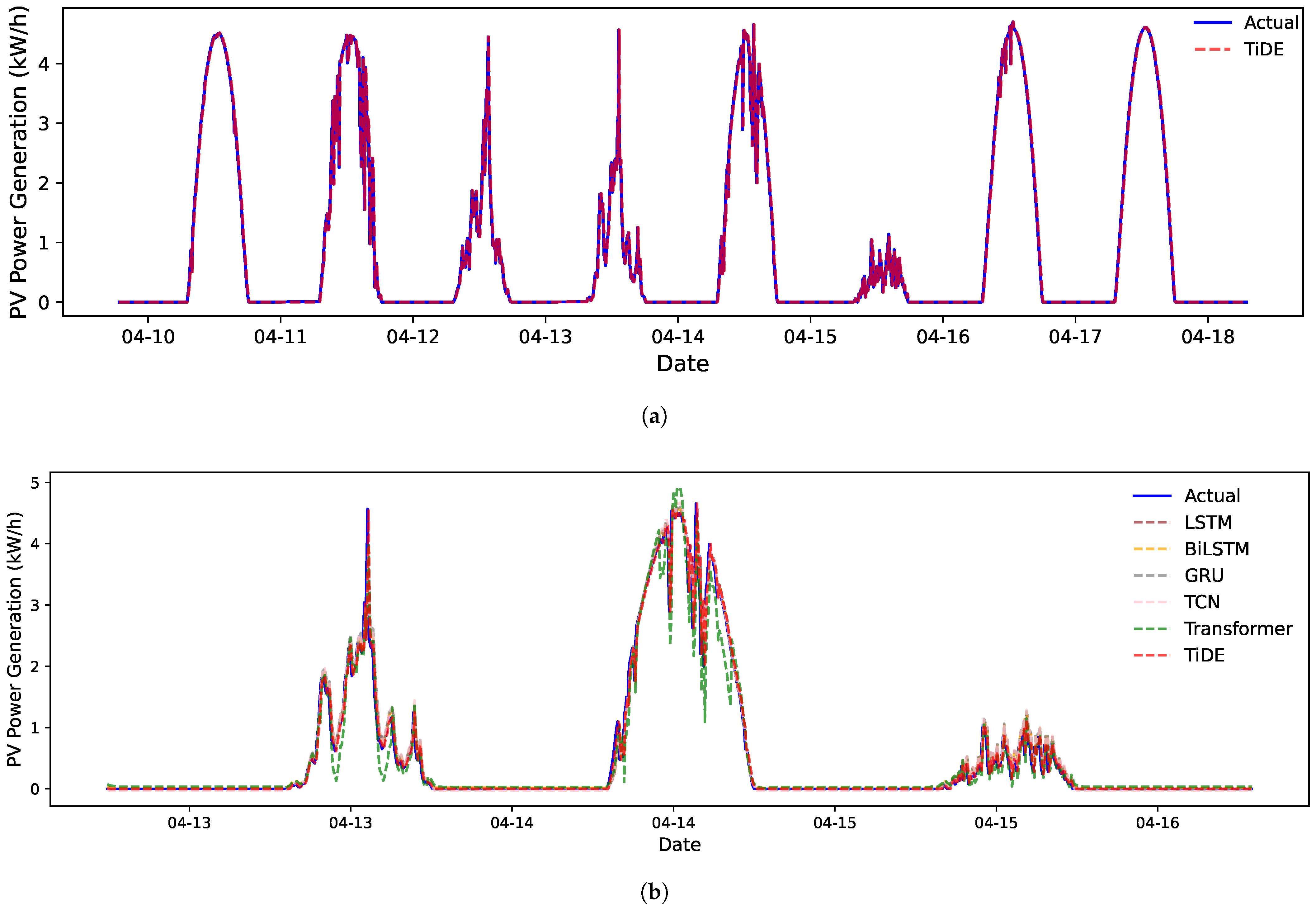
This study proposes a time-series dense encoder (TiDE)-based deep learning framework for photovoltaic (PV) power forecasting, addressing the challenges of nonlinear dependencies and computational inefficiencies in traditional methods. By integrating a multi-layer perceptron (MLP) encoder–decoder architecture with residual connections, TiDE can achieve high-precision predictions of PV power generation based on environmental variables. Using three years of operational data from a 5.4 kW PV system at DKASC for training and one year of data for testing, the TiDE model demonstrates good performance across varying time horizons and weather conditions.

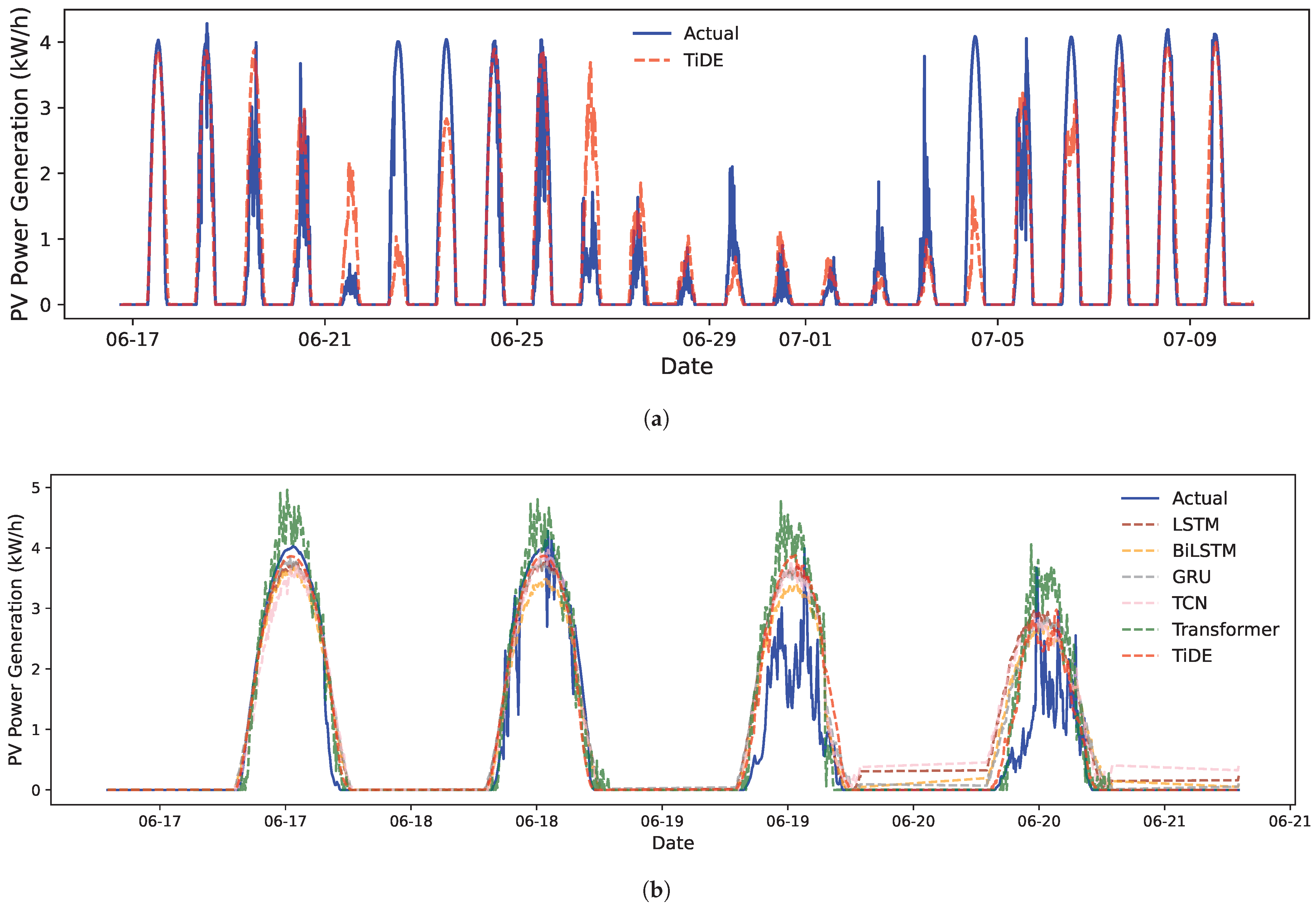
Key findings indicate that TiDE excels in short-term (5 min ahead) forecasts with R², MAE, and RMSE values of 0.952, 0.150, and 0.349, comparable to LSTM, GRU, and other models. However, its accuracy decreases for longer horizons, such as 1 h ahead forecasting, highlighting limitations in capturing abrupt environmental changes. Notably, TiDE shows superior adaptability in medium-term (1-day-ahead) forecasting, achieving the lowest MAE (0.507) among the compared models, particularly under complex meteorological conditions such as cloudy and rainy weather. Seasonal analysis further reveals its strengths in stable climates, such as autumn and winter, but also identifies challenges during extreme summer heat and spring dust storms, where RMSE values increase due to unmodeled nonlinear effects.

In this part of the discussion, our experiments show that the performance of the TiDE model is highly sensitive to extreme environmental conditions such as heavy rainfall, high humidity, overcast skies, and condensation scenarios, under which prediction accuracy significantly deteriorates. These limitations are mainly due to the scarcity of representative data samples and the exclusion of some relevant environmental variables. Nevertheless, TiDE shows promising generalizability across different PV systems and material types, as verified using an independent dataset from the Kaneka amorphous silicon system. While TiDE maintains competitive accuracy in short- and medium-term forecasts, its performance remains constrained by the underlying MLP structure. And from a business perspective, PV forecast errors threaten grid stability, increase market risks and costs, and require better models, real-time data, and coordinated energy management.

The innovation of TiDE lies in the introduction of time-intensive encoders, based on multi-layer perceptrons (MLPs), into PV power forecasting. By utilizing residual connections and staged encoding-decoding mechanisms, it effectively integrates both linear trends and nonlinear fluctuations, overcoming the trade-off between computational efficiency and complex dependency modeling found in traditional models. In comparison to recurrent models like LSTM and GRU, TiDE avoids the gradient vanishing/explosion problem and significantly reduces computational complexity. Compared to the Transformer, TiDE’s linear complexity enables real-time processing of high-frequency data and prevents GPU memory overload. Moreover, TiDE efficiently mitigates meteorological noise and retains critical trend information through dynamic covariate dimension reduction and global residual connections. This results in significantly lower MAE (0.791 and 0.962) under challenging weather conditions, such as cloudy and rainy days, and the best MAE (0.507) for 1-day forecasts. This design breaks free from the traditional reliance on attention mechanisms or convolutional structures for medium- and long-term predictions, offering a new paradigm that balances efficiency and robustness for the precise scheduling of PV systems.

The model’s accuracy in trend prediction makes it a viable tool for grid management and energy optimization. Future work could incorporate more environmental data, such as information on dust cover and extreme weather events like thunderstorms, to enhance the robustness and accuracy of predictions in specific geographic regions, such as tropical desert climates. These improvements could further solidify TiDE’s role in advancing renewable energy systems through reliable and scalable PV power forecasting. However, TiDE’s performance declines in the 1 h ahead forecast, suggesting that there is still room for structural improvement in the algorithm. Additional experiments based on the current framework could help refine the model and improve its predictive capabilities.

References

1. Parida, B.; Iniyan, S.; Goic, R. A review of solar photovoltaic technologies. Renew. Sustain. Energy Rev. 2011, 15, 1625–1636. [Google Scholar] [CrossRef]
2. Sampaio, P.G.V.; González, M.O.A. Photovoltaic solar energy: Conceptual framework. Renew. Sustain. Energy Rev. 2017, 74, 590–601. [Google Scholar] [CrossRef]
3. Electricity; IEA: Paris, France, 2025.
4. Ogliari, E.; Dolara, A.; Manzolini, G.; Leva, S. Physical and hybrid methods comparison for the day ahead PV output power forecast. Renew. Energy 2017, 113, 11–21. [Google Scholar] [CrossRef]
5. Li, Y.; He, Y.; Su, Y.; Shu, L. Forecasting the daily power output of a grid-connected photovoltaic system based on multivariate adaptive regression splines. Appl. Energy 2016, 180, 392–401. [Google Scholar] [CrossRef]
6. Hossain, M.S.; Wadi Al-Fatlawi, A.; Kumar, L.; Fang, Y.R.; Assad, M.E.H. Solar PV high-penetration scenario: An overview of the global PV power status and future growth. Energy Syst. 2024, 1868–2397. [Google Scholar] [CrossRef]
7. Kumar, L.; Khan, S.; Shaikh, F.; Siddiqui, M.M.; Sleiti, A.K. Enhanced deep-learning-based forecasting of solar photovoltaic generation for critical weather conditions. Clean Energy 2025, 9, 150–160. [Google Scholar] [CrossRef]
8. Ahmed, R.; Sreeram, V.; Mishra, Y.; Arif, M. A review and evaluation of the state-of-the-art in PV solar power forecasting: Techniques and optimization. Renew. Sustain. Energy Rev. 2020, 124, 109792. [Google Scholar] [CrossRef]
9. Wu, Y.-K.; Huang, C.-L.; Phan, Q.-T.; Li, Y.-Y. Completed review of various solar power forecasting techniques considering different viewpoints. Energies 2022, 15, 3320. [Google Scholar] [CrossRef]
10. Li, Q.Q.; Xu, Y.; Si, B.; Ding, H.Y.; Zhao, G.P. An integrated missing-data tolerant model for probabilistic PV power generation forecasting. IEEE Trans. Power Syst. 2022, 37, 4447–4459. [Google Scholar] [CrossRef]
11. Liu, J.; Zang, H.; Ding, T.; Chen, L.; Wei, Z.; Sun, G. Sky-image-derived deep decomposition for ultrashort-term photovoltaic power forecasting. IEEE Trans. Sustain. Energy 2023, 15, 871–883. [Google Scholar] [CrossRef]
12. Antonanzas, J.; Osorio, N.; Escobar, R.; Urraca, R.; Martinez-de-Pison, F.J.; Antonanzas-Torres, F. Review of photovoltaic power forecasting. Sol. Energy 2016, 136, 78–111. [Google Scholar] [CrossRef]
13. Louzazni, M.; Mosalam, H.; Khouya, A.; Amechnoue, K. A non-linear autoregressive exogenous method to forecast the photovoltaic power output. Sustain. Energy Technol. Assess. 2020, 38, 100670. [Google Scholar] [CrossRef]
14. AlShafeey, M.; Csáki, C. Evaluating neural network and linear regression photovoltaic power forecasting models based on different input methods. Energy Rep. 2021, 7, 7601–7614. [Google Scholar] [CrossRef]
15. Su, J.; Han, G.Y.; Shamai, S. Feedback Capacity of the Continuous-Time ARMA(1,1) Gaussian Channel. IEEE Trans. Inf. Theory 2024, 70, 6171–6188. [Google Scholar] [CrossRef]
16. Luzia, R.; Rubio, L.; Velasquez, C.E. Sensitivity analysis for forecasting Brazilian electricity demand using artiffcial neural networks and hybrid models based on Autoregressive Integrated Moving Average. Energy 2023, 274, 127365. [Google Scholar] [CrossRef]
17. Cunha, J.L.R.N.; Pereira, C.M.N.A. A hybrid model based on STL with simple exponential smoothing and ARMA for wind forecast in a Brazilian nuclear power plant site. Nucl. Eng. Des. 2024, 421, 113026. [Google Scholar] [CrossRef]
18. Das, U.L.; Tey, K.S.; Idris, M.Y.I.D.; Mekhilef, S.; Seyedmahmoudian, M.; Stojcevski, A.; Horan, B. Optimized Support Vector Regression-Based Model for Solar Power Generation Forecasting on the Basis of Online Weather Reports. IEEE Access 2022, 10, 15594–15604. [Google Scholar] [CrossRef]
19. Yang, Y.L.; Che, J.X.; Deng, C.Z.; Li, L. Sequential grid approach based support vector regression for short-term electric load forecasting. Appl. Energy 2019, 238, 1010–1021. [Google Scholar] [CrossRef]
20. Ahmad, M.W.; Mourshed, M.; Rezgui, Y. Tree-based ensemble methods for predicting PV power generation and their comparison with support vector regression. Energy 2018, 164, 465–474. [Google Scholar] [CrossRef]
21. Wang, J.; Li, P.; Ran, R.; Che, Y.; Zhou, Y. A short-term photovoltaic power prediction model based on the gradient boost decision tree. Appl. Sci. 2018, 8, 689. [Google Scholar] [CrossRef]
22. Ramkumar, G.; Sahoo, S.; Amirthalakshmi, T.; Ramesh, S.; Prabu, R.T.; Kasirajan, K.; Samrot, A.V.; Ranjith, A. A short-term solar photovoltaic power optimized prediction interval model based on FOS-ELM algorithm. Int. J. Photoenergy 2021, 2021, 3981456. [Google Scholar] [CrossRef]
23. Chen, C.; Duan, S.; Cai, T.; Liu, B. Online 24-h solar power forecasting based on weather type classiffcation using artiffcial neural network. Sol. Energy 2011, 85, 2856–2870. [Google Scholar] [CrossRef]
24. Almonacid, F.; Pérez-Higueras, P.; Fernández, E.F.; Hontoria, L. A methodology based on dynamic artiffcial neural network for short-term forecasting of the power output of a PV generator. Energy Convers. Manag. 2014, 85, 389–398. [Google Scholar] [CrossRef]
25. Vaz, A.; Elsinga, B.; Van Sark, W.; Brito, M. An artiffcial neural network to assess the impact of neighbouring photovoltaic systems in power forecasting in Utrecht, the Netherlands. Renew. Energy 2016, 85, 631–641. [Google Scholar] [CrossRef]
26. Wang, K.; Qi, X.; Liu, H. A comparison of day-ahead photovoltaic power forecasting models based on deep learning neural network. Appl. Energy 2019, 251, 113315. [Google Scholar] [CrossRef]
27. Jung, Y.; Jung, J.; Kim, B.; Han, S. Long short-term memory recurrent neural network for modeling temporal patterns in long-term power forecasting for solar PV facilities: Case study of South Korea. J. Clean. Prod. 2020, 250, 119476. [Google Scholar] [CrossRef]
28. Huang, X.; Li, Q.; Tai, Y.; Chen, Z.; Liu, J.; Shi, J.; Liu, W. Time series forecasting for hourly photovoltaic power using conditional generative adversarial network and Bi-LSTM. Energy 2022, 246, 123403. [Google Scholar] [CrossRef]
29. Yu, Y.; Cao, J.; Zhu, J. An LSTM short-term solar irradiance forecasting under complicated weather conditions. IEEE Access 2019, 7, 145651–145666. [Google Scholar] [CrossRef]
30. Chen, Y.; Li, X.; Zhao, S. A Novel Photovoltaic Power Prediction Method Based on a Long Short-Term Memory Network Optimized by an Improved Sparrow Search Algorithm. Electronics 2024, 13, 993. [Google Scholar] [CrossRef]
31. Min, H.; Hong, S.; Song, J.; Son, B.; Noh, B.; Moon, J. SolarFlux Predictor: A Novel Deep Learning Approach for Photovoltaic Power Forecasting in South Korea. Electronics 2024, 13, 2071. [Google Scholar] [CrossRef]
32. Moon, J. A Multi-Step-Ahead Photovoltaic Power Forecasting Approach Using One-Dimensional Convolutional Neural Networks and Transformer. Electronics 2024, 13, 2007. [Google Scholar] [CrossRef]
33. Radhi, S.M.; Al-Majidi, S.D.; Abbod, M.F.; Al-Raweshidy, H.S. Machine Learning Approaches for Short-Term Photovoltaic Power Forecasting. Energies 2024, 17, 4301. [Google Scholar] [CrossRef]
34. Jing, S.; Xi, X.; Su, D.; Han, Z.; Wang, D. Spatio-Temporal Photovoltaic Power Prediction with Fourier Graph Neural Network. Electronics 2024, 13, 4988. [Google Scholar] [CrossRef]
35. Das, A.; Kong, W.; Leach, A.; Mathur, S.; Sen, R.; Yu, R. Long-term forecasting with tide: Time-series dense encoder. arXiv 2023, arXiv:2304.08424. [Google Scholar]
36. Zeng, A.; Chen, M.; Zhang, L.; Xu, Q. Are transformers effective for time series forecasting? In Proceedings of the AAAI Conference on Artificial Intelligence, Washington, DC, USA, 7–14 February 2023; Volume 37. [Google Scholar]
37. Hochreiter, S.; Schmidhuber, J. Long short-term memory. Neural Comput. 1997, 9, 1735. [Google Scholar] [CrossRef] [PubMed]
38. Graves, A.; Mohamed, A.R.; Hinton, G. Speech recognition with deep recurrent neural networks. In Proceedings of the 2013 IEEE International Conference on Acoustics, Speech and Signal Processing, Vancouver, BC, Canada, 26–31 May 2013; Volume 6645. [Google Scholar]
39. Chung, J.; Gulcehre, C.; Cho, K.; Bengio, Y. Empirical evaluation of gated recurrent neural networks on sequence modeling. arXiv 2014, arXiv:1412.3555. [Google Scholar]
40. Lea, C.; Flynn, M.D.; Vidal, R.; Reiter, A.; Hager, G.D. Temporal convolutional networks for action segmentation and detection. In Proceedings of the IEEE Conference on Computer Vision and Pattern Recognition, Honolulu, HI, USA, 21–26 July 2017; pp. 156–165. [Google Scholar]
41. Han, K.; Wang, Y.; Chen, H.; Chen, X.; Guo, J.; Liu, Z.; Tang, Y.; Xiao, A.; Xu, C.; Xu, Y.; et al. A survey on vision transformer. IEEE Trans. Pattern Anal. Mach. Intell. 2022, 45, 87–110. [Google Scholar] [CrossRef]
Figure 1. The architecture of TiDE. The orange part represents the target set for prediction, and the blue is the process for dynamic covariates. The green part gives the ncoder process, and the red shows the decoder. The gray part is the output prediction.
Energies 18 02434 g001
Figure 2. The details of the residual block.
Energies 18 02434 g002
Figure 3. (a) The 5 min ahead PV power generation forecasting of TiDE from 10 to 18 April 2023; (b) the comparison of 5 min ahead PV power generation forecasting for different algorithms from 13 to 16 April 2023.
Energies 18 02434 g003
Figure 4. (a) The 5 min ahead PV power generation forecasting of TiDE from 17 June to 9 July 2023; (b) a comparison of 5 min ahead PV power generation forecasting values for different algorithms from 17 to 21 June.
Energies 18 02434 g004