Teager–Kaiser Energy Operator-Based Short-Circuit Fault Localization Method for Multi-Circuit Parallel Cables

Abstract

Medium-voltage cables in hydropower plants are typically arranged in multi-circuit configurations to ensure reliability, yet their exposure to harsh operational conditions accelerates insulation degradation and increases partial discharge risks. Traditional fault localization methods, such as the traveling wave method using wavelet transform to process fault signals, suffer from wavefront distortion due to inter-line reflections and noise interference in multi-circuit systems, because wavelet-based techniques are limited by preset basis functions and environmental noise. To address these challenges, a fault localization method for multi-circuit parallel cables based on the Teager–Kaiser Energy Operator (TKEO) is proposed in this paper. First, the fault signal is decoupled using Clarke transformation to suppress common-mode interference, obtaining the α component. Subsequently, the α component is subjected to wavelet transform to obtain the high-frequency components, which are then optimized using the TKEO. The TKEO is applied to optimize the wavelet-transformed signal, enhancing transient energy variations to precisely identify the arrival time of the fault wavefront at measurement points, thereby enabling accurate fault localization. The results of the four types of fault experiments indicate that the use of the TKEO to optimize the wavelet transform of the traveling wave method improved the accuracy of fault localization.

1. Introduction

As critical infrastructures for renewable energy generation, hydropower plants require ultra-reliable auxiliary power systems. Cable failures in these systems not only cause unplanned downtime but may also lead to cascading outages that threaten grid stability [1]. In hydropower plants, power cables are essential components of the auxiliary power distribution network. With the increasing capacity of hydro-generating units and the intelligent upgrades of auxiliary equipment, the demand for reliability and redundancy in the power supply continues to grow. To meet high reliability requirements, multi-circuit parallel cable operation has become a core strategy in hydropower plants to enhance power supply capacity and achieve load balancing [2]. Compared to overhead lines, medium-voltage cables in hydropower plants are typically installed in underground tunnels or enclosed cable trays, providing advantages in spatial adaptability and resistance to harsh environmental conditions. However, prolonged exposure to humid environments, mechanical vibrations, and electromagnetic coupling accelerates insulation aging, moisture ingress, and partial discharge [3]. Statistical data indicate that defects such as cable joint oxidation and sheath damage account for over 35% of electrical faults in hydropower plants [4]. Nevertheless, due to concealed cable routing and the complex electromagnetic interference in multi-circuit parallel systems, fault localization accuracy is often hindered by challenges such as traveling wave signal attenuation and mode aliasing [5,6,7]. Therefore, developing high-precision fault localization methods tailored to multi-circuit parallel cables in hydropower plants is essential in ensuring the safe operation of generating units and the continuous supply of auxiliary power.

Currently, cable fault localization methods primarily include impedance-based and traveling wave-based approaches. Impedance-based techniques, such as the bridge method and high-resistance fault method, measure fault distances by analyzing impedance changes. For instance, the bridge method proposed connects the faulted phase and a non-faulted phase as two arms of a Wheatstone bridge, with adjustable resistors forming the other arms [8]. By balancing the bridge, the fault impedance is measured to calculate the fault distance. However, this method struggles with high-resistance faults due to insufficient current for accurate measurements. To address this, a high-resistance fault method that applies a high voltage is introduced to convert high-resistance faults into low-resistance states, enabling fault distance calculation using the distributed parameter line theory [9]. Traveling wave methods are primarily classified into single-ended and double-ended localization methods [10]. The single-ended traveling wave method offers advantages such as lower equipment requirements and simpler operation; however, in multi-circuit parallel cable systems, mutual interference between traveling wave signals significantly compromises the accurate detection of wavefront arrival times, thereby introducing substantial measurement errors [11]. In contrast, the double-ended traveling wave method achieves a qualitative enhancement in localization accuracy, noise immunity, and adaptability to complex network topologies—albeit at the cost of increased economic investment, making it particularly suitable for multi-circuit parallel cable configurations. Single-ended traveling wave detection, while cost-effective and simple, cannot reliably resolve overlapping wavefronts from parallel cables, leading to significant errors [12,13]. In contrast, double-ended methods calculate fault distances using time differences between wavefront arrivals at both ends of the cable but require synchronized measurements and complex signal processing [14].

Despite their widespread use, both the impedance and traveling wave methods face limitations in signal extraction accuracy and noise susceptibility [15]. Wavelet transform, known for its ability to extract localized signal features, has been applied in power system disturbance detection [16]. While effective in amplifying transient fault characteristics, it struggles with precise feature extraction in multi-circuit environments due to noise interference and predefined basis function constraints [17]. A method integrating Variational Mode Decomposition (VMD) into the Teager–Kaiser Energy Operator (TKEO) is proposed for rolling bearing fault diagnosis to improve the TKEO’s capability to enhance transient energy features in low signal-to-noise scenarios [13,18,19,20].

Based on existing research, this paper proposes a TKEO-based fault localization method to tackle the issue of inaccurate fault location in multi-circuit parallel cable short circuits using the traveling wave method. First, a fault model is constructed by analyzing the multi-circuit parallel cables. Additionally, by integrating Clarke’s transformation for signal decoupling with TKEO-optimized wavelet processing, an approach that suppresses electromagnetic interference and accurately identifies wavefront arrival times is examined. Finally, the effectiveness of the proposed method is validated through the simulation analysis of four different short-circuit fault cases.

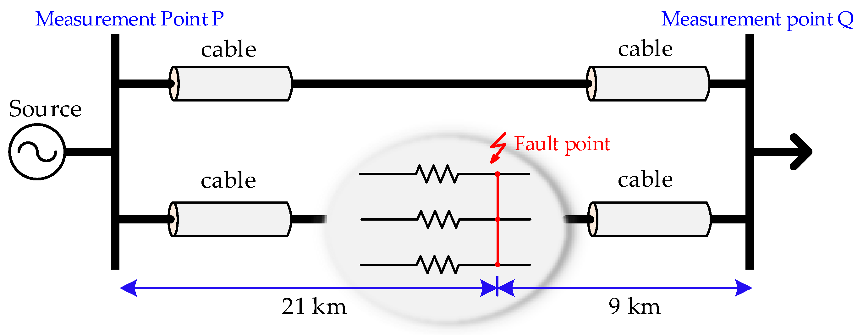
2. Model of Multi-Circuit Parallel Cables and Fault Localization Method

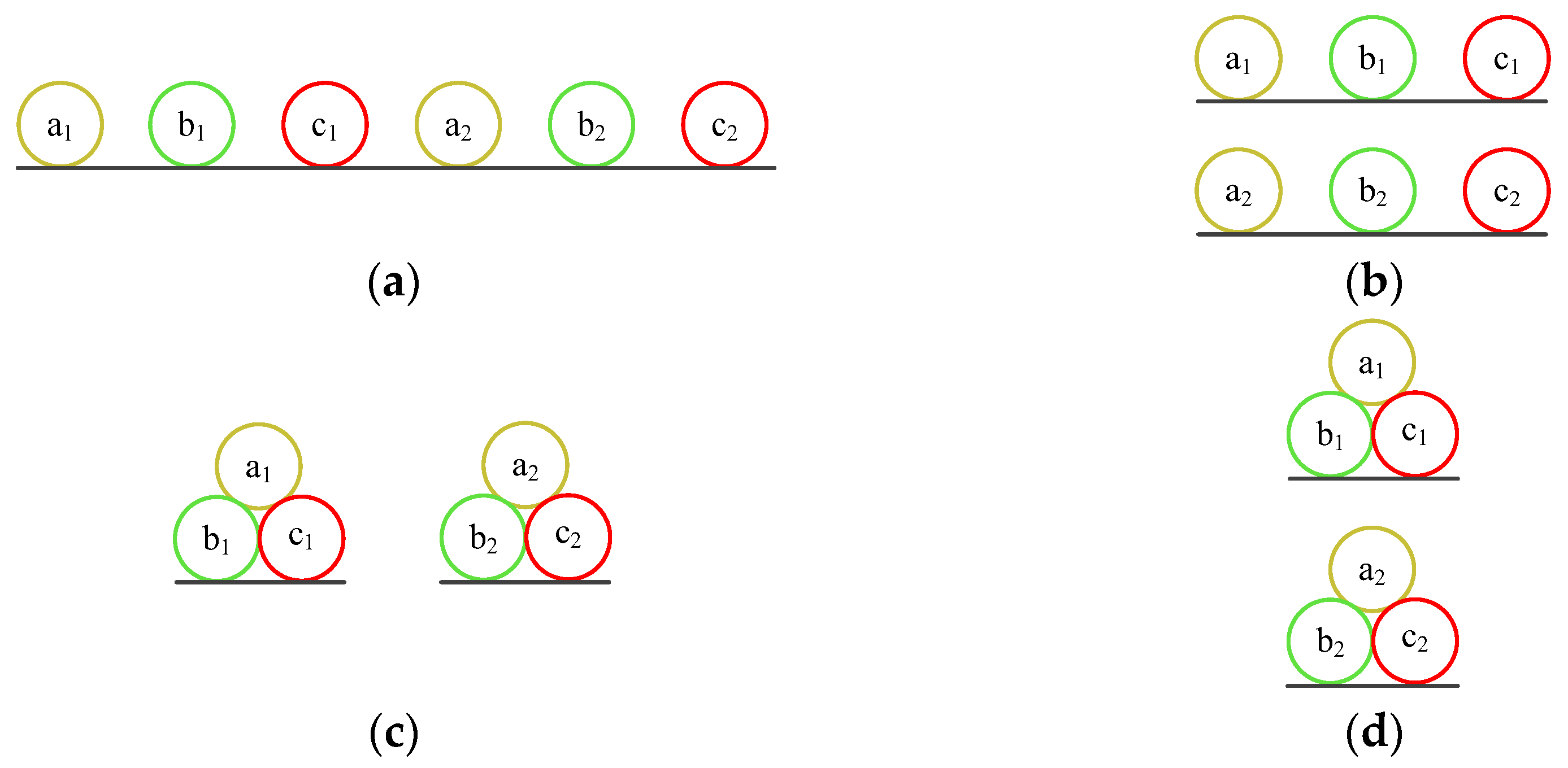
2.1. Multi-Circuit Cable Installation Methods and Asymmetry Analysis

For high-power electrical equipment, traditional three-core cables may not sufficiently meet load demands. Therefore, single-core cables arranged in parallel are widely adopted. This approach not only fulfills power requirements but also offers advantages such as ease of installation, shortened construction periods, and space efficiency. The flexibility of single-core parallel installations enhances the overall construction efficiency while enabling high-capacity power transmission within confined spaces. Figure 1 depicts the basic structure of single-core cables, while Figure 2 presents four common installation methods for double-circuit parallel cable systems.

Although multi-circuit parallel configurations enhance power transmission capacity, inconsistent cable impedance may arise due to variations in inter-phase distances and mutual inductance between phases. To quantify this effect, the zero-sequence asymmetry degree B₀ and negative-sequence through-type asymmetry degree B₂ are defined as follows.

$$\begin{array}{l}{B}_0={\displaystyle \frac{I_0^{\mathrm{I}}+I_0^{\mathrm{II}}}{I_1^{\mathrm{I}}+I_1^{\mathrm{II}}}}\\ B_2={\displaystyle \frac{I_2^{\mathrm{I}}+I_2^{\mathrm{II}}}{I_1^{\mathrm{I}}+I_1^{\mathrm{II}}}}\end{array}$$

(1)

where I₀^I and I₀^II are the zero sequence currents in the first and second circuits, respectively. I₁^II and I₁^II are the positive sequence currents in the first and second circuits, respectively. I₂^II and I₂^II are the negative sequence currents in the first and second circuits, respectively.

Among the four installation methods, the triangular vertical arrangement (Figure 2d) exhibits the lowest asymmetry degrees, with B₀ = 0.59% and B₂ = 0.5%. In this configuration, the current waveforms of the double-circuit cables align closely, and both B₀ and B₂ remain below 0.6%. Consequently, the asymmetry effects can be considered negligible when adopting the triangular vertical arrangement.

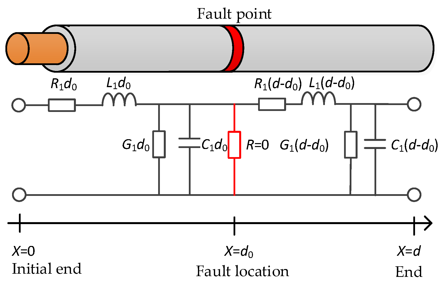
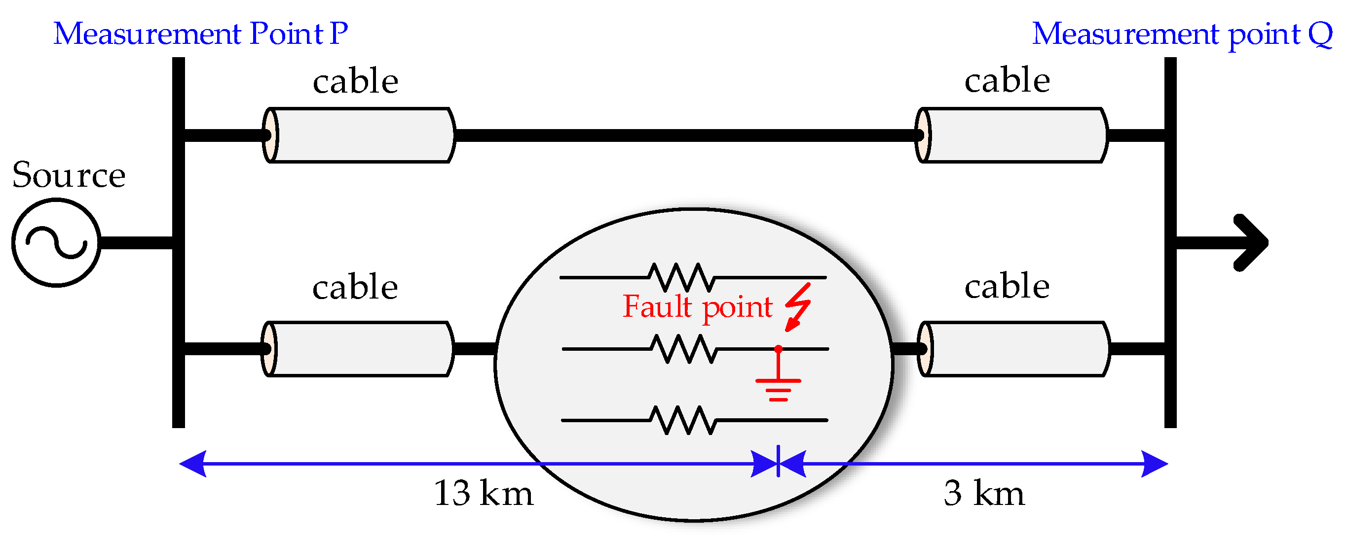
2.2. Short-Circuit Fault Model of Cable

When a short-circuit fault occurs in a power cable, the grounding resistance at the fault point is ideally close to zero under theoretical conditions. The equivalent circuit model of the cable is illustrated in Figure 3.

Under high-frequency operating conditions, the inductive reactance dominates the resistance, and the susceptance is significantly larger than the conductance. Consequently, the characteristic impedance can be approximated as

$$Z=\sqrt{{\displaystyle \frac{R_1+j\omega L_1}{G_1+j\omega C_1}}}=\sqrt{{\displaystyle \frac{L_1}{C_1}}}$$

(2)

During a cable fault, a sudden voltage collapse occurs at the fault point, initiating an electric arc. This transient event generates traveling waves propagating along the cable. The velocity of the traveling waves v is determined by the cable’s distributed parameters.

$$v=1/\sqrt{L_1{C}_1}$$

(3)

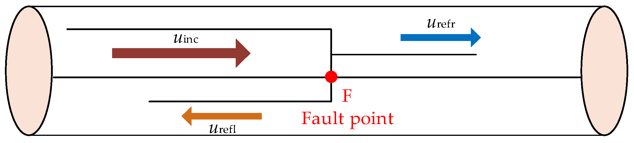
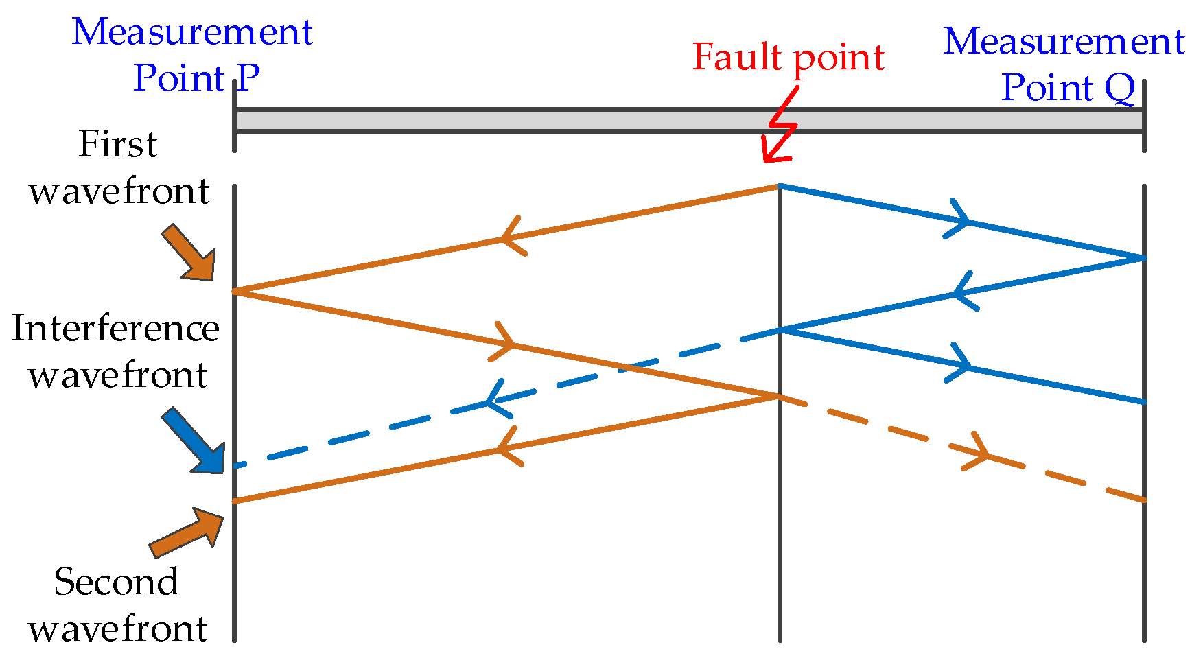
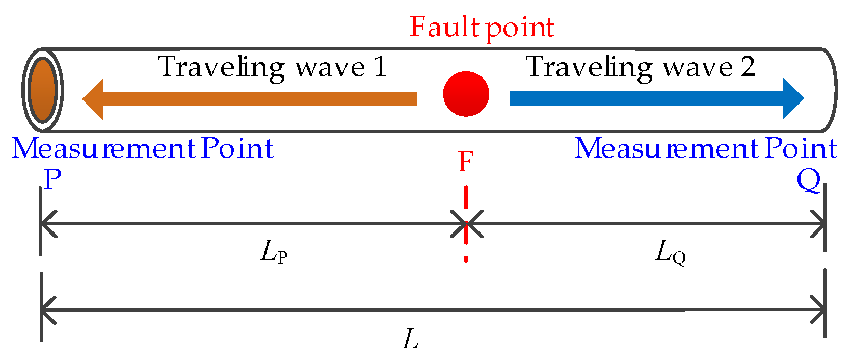
2.3. Fault Localization Method in Multi-Circuit Parallel Cables

The traveling wave method, as a primary technique for fault localization in power cables, operates based on the characteristic differences between steady-state and transient behaviors: under normal operation, cables transmit standard sinusoidal waveforms, whereas faults induce abrupt electromagnetic field variations that generate transient traveling wave signals. These signals propagate between the fault point and busbars through refraction and reflection processes, with their voltage waveforms serving as the critical features for precise fault localization.

Figure 4 illustrates the schematic diagram of traveling wave refraction and reflection, where u_inc, u_refl, and u_refr denote the incident wave, reflected wave, and refracted wave, respectively, with F marking the fault localization.

In the traveling wave method, once the cable material parameters are determined, the wave propagation velocity can be approximated as a constant. Leveraging this property, the fault distance is calculated through the linear relationship between the wave propagation time delay and velocity. Currently, the methodologies are primarily classified into single-ended and double-ended localization methods. When employing the conventional single-ended traveling wave localization method, significant challenges arise in multi-circuit parallel cable configurations experiencing simultaneous fault conditions. Each discrete fault point initiates characteristic wavefronts that subsequently interact with impedance discontinuities through successive reflection and refraction phenomena. This wave superposition creates complex signal interference patterns at the measurement terminal, particularly compromising the discernibility of correlated wavefront signatures originating from a common fault source, as shown in Figure 5. Consequently, traditional single-ended traveling wave analysis demonstrates fundamental limitations in achieving reliable fault discrimination and precise localization within multi-conductor parallel cable systems.

Compared with the single-ended traveling wave ranging method, which has the disadvantage of overlapping reflected and refracted waves, the double-ended traveling wave ranging method has obvious advantages in fault location in multi-branch cables. It determines the fault localization by measuring the time difference in wave arrivals at both cable ends, as shown in Figure 6.

We assume the fault occurs at point F on line PQ, which has a total length of L. L_p and L_Q denote the distances from F to P and Q, respectively. t_P and t_Q are the wave arrival times at P and Q, respectively. v is the wave propagation speed. Based on wave propagation principles, the fault distance can be expressed as

$$\left\{\begin{array}{l}{L}_{\mathrm{P}}+L_{\mathrm{Q}}=L\\ {\displaystyle \frac{L_{\mathrm{P}}}{v}}-{\displaystyle \frac{L_{\mathrm{Q}}}{v}}=t_{\mathrm{P}}-t_{\mathrm{Q}}\end{array}\right.$$

(4)

Then,

$$\left\{\begin{array}{l}{L}_{\mathrm{P}}={\displaystyle \frac{1}{2}}\left[L+v\left(t_{\mathrm{P}}-t_{\mathrm{Q}}\right)\right]\\ L_{\mathrm{Q}}={\displaystyle \frac{1}{2}}\left[L+v\left(t_{\mathrm{Q}}-t_{\mathrm{P}}\right)\right]\end{array}\right.$$

(5)

The double-ended ranging method utilizes the initial wavefront detection at both terminal measurement points, effectively circumventing the interference from subsequent reflection and refraction phenomena through time-domain signal discrimination, thereby demonstrating particular efficacy in multi-circuit parallel cables with concurrent fault scenarios. To quantitatively assess the localization accuracy enhancement, the optimization degree Δ is defined as

$$\Delta ={\displaystyle \frac{\left|\left|X_{\mathrm{k}}-X_0\right|-\left|X_c-X_0\right|\right|}{\left|X_c-X_0\right|}}$$

(6)

where X_k is the fault localization result using TKEO optimization, X_c is the result using traditional methods, and X₀ is the distance from the fault point to the measurement end.

3. Improved Short-Circuit Fault Localization Method

3.1. Conventional Wavelet Transform Method

The wavelet transform method, featuring multi-resolution analysis, is adept at capturing local signal characteristics, thereby rendering it ideal for fault diagnosis. Its essence lies in the comparison of a fixed basis function with the signal, thereby constructing a family of functions.

The wavelet transform basis is defined as

$${\Phi }_{u,v}\left(t\right)={\displaystyle \frac{1}{\sqrt{\left|u\right|}}}\Phi \left({\displaystyle \frac{t-v}{u}}\right)$$

(7)

where u is the scaling factor, v is the translation factor, and Φ is the mother wavelet function. The continuous wavelet transform of a signal f(t) is

$$W_f(u,v)={\displaystyle \frac{1}{\sqrt{\left|u\right|}}}{\displaystyle {\int }_{-\infty }^{+\infty }f(t)\overline{\Phi (\frac{t-v}{u}}})\mathrm{d}t$$

(8)

Different scaling factors u change the signal’s frequency, similarly to bandpass filtering. The wavelet transform decomposes a signal into low-frequency approximations and high-frequency details, with the latter aiding in detecting signal mutations.

Define a function at scale u such that, within the neighborhood of v₀, for any v₀ ∈ (v₀ − δ, v₀ + δ), it always holds that

$$\left|W_f\left(u,v\right)\right|\le \left|W_f\left(u,v_0\right)\right|$$

(9)

where v₀ is the modulus maximum point of the wavelet function and is the modulus maximum value of the wavelet transform.

In the wavelet transform domain, the modulus maxima points correspond to the time instants at which the fault signal reaches the measurement point. Thus, fault localization can be transformed into finding these modulus maxima points in the wavelet transform results.

In this paper, the Discrete Wavelet Transform (DWT) combined with the Daubechies 4th-order wavelet (db4) is employed to decompose traveling wave signals. The compact support and orthogonality of the db4 wavelet enable it to effectively match the transient characteristics of traveling wavefronts. Through a 3-level decomposition, high-frequency noise is separated from effective signal components. The first-level detail coefficients (D1) are selected for subsequent energy analysis, as their coverage of the 500 kHz–1 MHz frequency band closely aligns with the energy distribution of traveling wavefronts.

3.2. Teager–Kaiser Energy Operator

The TKEO is primarily used to highlight the relationship between the amplitude and frequency of a signal, effectively reflecting signal mutations. For continuous signals, the TKEO is defined as follows:

$$\Psi \left[r\left(t\right)\right]={[r^{\prime }\left(t\right)]}^2-r\left(t\right)r^{″}\left(t\right)$$

(10)

where $r^{\prime }\left(t\right)$ and $r^{″}\left(t\right)$ are the first- and second-order derivatives of the signal with respect to time.

For a discrete signal r(n), it can be defined as

$$\left\{\begin{array}{l}r(n)=A\cos (\omega n+\theta )\\ \omega =2\mathsf{\pi }f/f_0\end{array}\right.$$

(11)

where A is the amplitude, f is the frequency of the discrete signal r(n), f₀ is the sampling frequency, and θ is the initial phase of r(n). A, ω, and θ can be determined by setting up the following system of equations using three consecutive signal points.

$$\left\{\begin{array}{l}r(n-1)=A\cos [\omega (n-1)+\theta ]\\ r(n)=A\cos (\omega n+\theta )\\ r(n+1)=A\cos [\omega (n+1)+\theta ]\end{array}\right.$$

(12)

By solving equation set (12), we can obtain

$${[r(n)]}^2-r(n-1)r(n+1)=A^2{\sin }^2(\omega )$$

(13)

When the sampling frequency is sufficiently high, the approximation ω ≈ sin(ω) holds true, leading to

$${[r(n)]}^2-r(n-1)r(n+1)=A^2{\omega }^2$$

(14)

So, the TKEO for discrete signals is defined as

$$\begin{array}{cc}\hfill \Psi \left[r\left(n\right)\right]& ={[r(n)]}^2-r(n-1)r(n+1)\hfill \\ & =A^2{\omega }^2\hfill \end{array}$$

(15)

The TKEO effectively captures the instantaneous components of signal energy mutation when analyzing harmonic signals. Based on this, the TKEO can effectively analyze wavelet signals and accurately determine the moment when the fault-traveling wavefront reaches the measurement section.

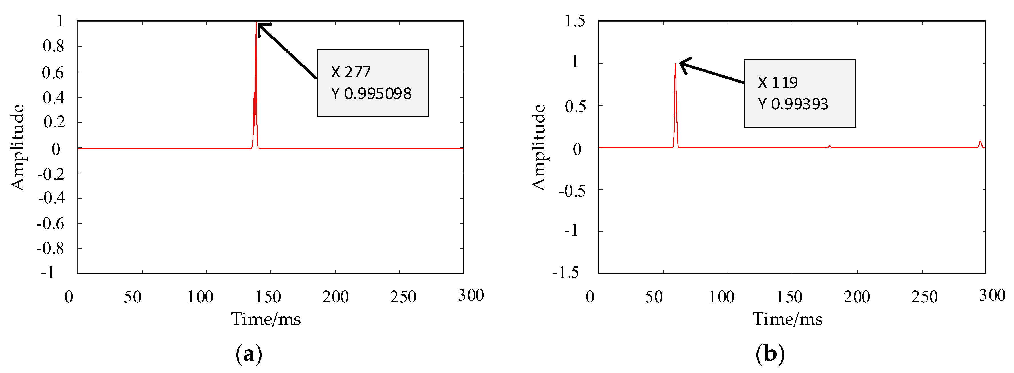
3.3. Short-Circuit Fault Localization Method Based on TKEO

Incorporating the TKEO algorithm, a signal processing method for power cable short-circuit fault location is proposed in this paper. The specific steps of this method are illustrated in Figure 7.

The process initiates with the construction of a cable simulation model to extract voltage signals from both the bus and line ends, followed by the computation of the transient component of the voltage mutation value. Upon acquiring these values, the Clarke transformation is employed to decouple the voltage components. The decoupled voltage magnitudes are then subjected to wavelet transform analysis. Subsequently, the TKEO is utilized to enhance the high-frequency wavelet components and extract the optimized modulus maxima. Ultimately, the fault location is ascertained by analyzing the time difference in the first-arriving traveling wave wavefronts at both cable ends.

4. Accuracy Verification

In order to verify the accuracy of the proposed method in this paper, four different types of short-circuit fault simulations were conducted on a double-circuit parallel cable in this chapter. The signal sampling frequency is 2 MHz. The cable parameters are shown in

Table 1. Cable parameters in all cases.

Cable Parameters	Value	Unit
Positive Sequence Resistance	0.0127	Ω/km
Zero Sequence Resistance	0.3864	Ω/km
Positive Sequence Inductance	0.2230	mH/km
Zero Sequence Inductance	0.8911	mH/km
Positive Sequence Capacitance	190.680	nF/km
Zero Sequence Capacitance	190.660	nF/km

. This case is a detailed fault location process, while the other three cases are provided to demonstrate the applicability of the method. Due to space limitations, repetitive descriptions are omitted.

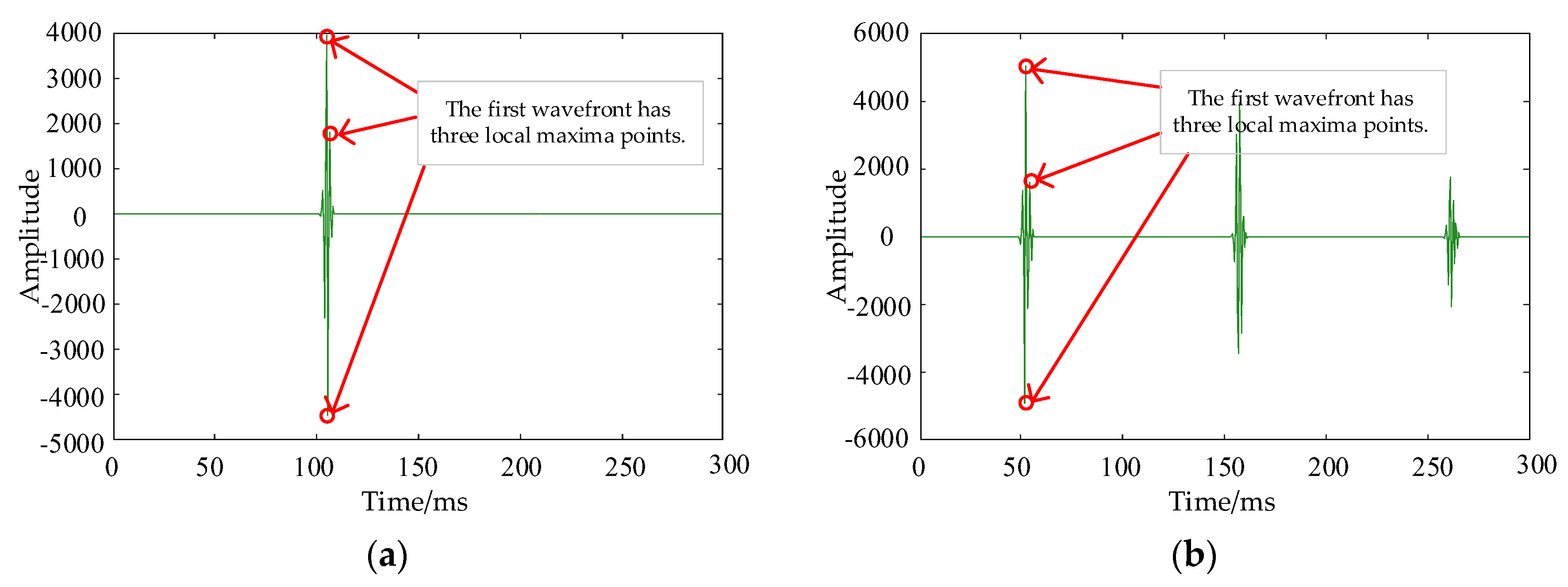
4.1. Single-Phase Grounding Fault Localization Case

Before performing fault localization, the voltage signals at the measurement points at both ends of the cable are first extracted and compared with the voltage under normal operating conditions. By analyzing the voltage fluctuations, it is possible to determine whether there are any abnormal variations. When the amplitude of the voltage fluctuation exceeds a set threshold, it can be preliminarily determined that there may be a fault in the cable line, which then triggers the subsequent fault localization process.

Firstly, a single-phase grounding fault is simulated in this case. The entire cable is 16 km long, and the fault point is set at a distance of 13 km from measurement point P and 3 km from measurement point Q. The fault time is set at 20 ms. The simulation model is shown in Figure 8.

Figure 9 shows the voltage waveforms of the three phases where a voltage mutation can be observed at the 20 ms time point, indicating the presence of a fault in the cable. Therefore, to detect whether a fault has occurred, the voltage difference between adjacent sampling points is used for judgment. If the voltage difference exceeds the preset value, it is considered that a fault exists in the line. The voltage difference waveform is shown in Figure 10. In Figure 9, Figure 10 and Figure 11, The blue line represents the voltage of Phase A, the yellow line represents the voltage of Phase B, and the red line represents the voltage of Phase C.

Figure 11 shows the transient voltage waveform after the Clarke transformation.

Firstly, the voltage signals are collected at both measurement points P and Q. Then, the Clarke transformation is used to decouple the transient voltage components and to highlight the fault characteristics. Based on the decoupled alpha modulus, we perform a three-level wavelet decomposition using the db4 wavelet transform and select the high-frequency component D1. The high-frequency components during the fault are shown in Figure 12.

As shown in Figure 12, the signal energy changes significantly when the fault-traveling wavefront reaches the measurement point. According to the modulus maximum principle, the sampling point at the time of fault can be accurately determined. However, the results in Figure 12 show that the first wavefront has three local maxima points. The wavelet transform failed to capture the accurate fault moment, leading to fault localization errors. Therefore, to improve localization accuracy, optimization using the TKEO is needed.

Optimizing Figure 12 with the TKEO yields the waveform shown in Figure 13.

The modulus maxima points can be determined based on Figure 12. By applying the TKEO optimization method to signals at both points P and Q, the precise sampling points corresponding to the arrival of fault-induced traveling wavefronts at these terminals are identified. Finally, the fault localization is calculated using the ranging Formula (5).

According to Formula (6), the fault localization optimization degree Δ for the data in

Table 2. Localization results for single-phase grounding faults.

Actual Fault Distance/km	Ranging Method	Localization Results/km	Relative Error/%
10	Without Using TKEO	10.1086	1.0860
	Using TKEO	10.0319	0.3190
11	Without Using TKEO	10.9137	−0.7845
	Using TKEO	10.9904	−0.0873
12	Without Using TKEO	12.1022	0.8517
	Using TKEO	12.0639	0.5325
13	Without Using TKEO	13.0607	0.4669
	Using TKEO	13.0223	0.1858

is calculated as 70.63%, 88.83%, 37.47%, and 63.24%, with an average optimization degree of 65.04%.

4.2. Two-Phase Grounding Fault Localization Case

In order to validate the universality of the proposed fault localization method, a two-phase grounding fault is further studied with identical cable parameters to those in Table 1. In this case, the entire cable is 24 km long. And the fault point is located at 16 km and 8 km from the measurement points P and Q, respectively. The specific two-phase grounding fault simulation diagram is shown in Figure 14.

As in the single-phase grounding fault localization case, the voltage transient components at both ends of the measurement points are extracted in this case. Then, they are decoupled through the Clarke transformation and then subjected to wavelet transformation, as depicted in Figure 15.

Then, the TKEO optimization method is applied to process the waveforms and further enhance the fault localization accuracy, as shown in the waveform diagram in Figure 16.

Finally, the fault localization is calculated using the ranging Formula (5).

Table 3. Localization results for two-phase grounding faults.

Actual Fault Distance/km	Ranging Method	Localization Results/km	Relative Error/%
14	Without Using TKEO	14.1086	0.7757
	Using TKEO	14.0319	0.2279
16	Without Using TKEO	16.1022	0.6388
	Using TKEO	16.0255	0.1594
18	Without Using TKEO	18.0958	0.5322
	Using TKEO	18.0191	0.1061
20	Without Using TKEO	20.0894	0.4470
	Using TKEO	20.0511	0.2555

compares the fault localization results with and without TKEO optimization.

According to Formula (6), the fault localization optimization degree Δ for the data in Table 3 is calculated as 70.63%, 75.05%, 80.06%, and 42.84%, with an average optimization degree of 67.15%.

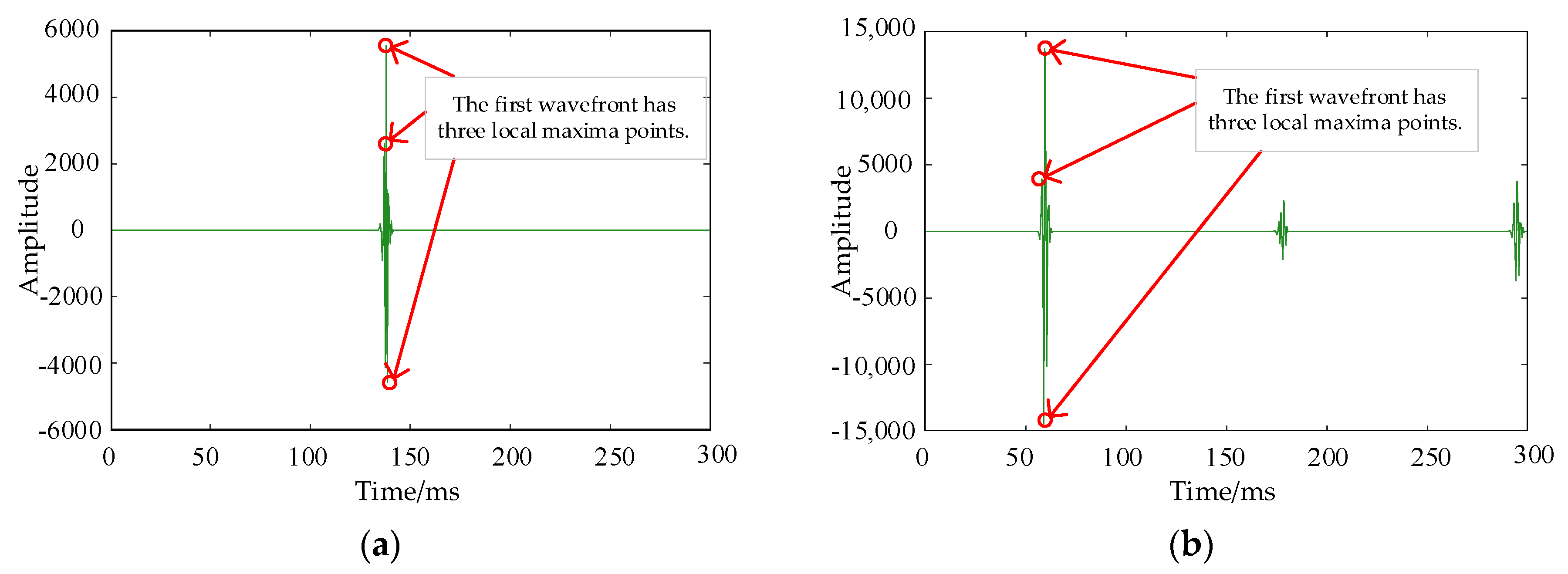
4.3. Two-Phase Short-Circuit Fault Localization Case

Furthermore, two-phase short-circuit fault simulation is taken into consideration. In this case, the entire cable is 24 km long, and the fault point is 16 km from the measurement point P and 8 km from point Q. Its simulation model is shown in Figure 17.

The voltage transient components at both the measurement points P and Q are extracted, decoupled via Clarke transformation, and then subjected to wavelet transformation. The results are shown in Figure 18.

Then, the TKEO optimization method is applied to process the waveforms, further enhancing the fault localization accuracy, as shown in the waveform diagram in Figure 19.

Finally, the fault localization is calculated using the ranging Formula (5).

Table 4. Localization results for two-phase short-circuit fault.

Actual Fault Distance/km	Ranging Method	Localization Results/km	Relative Error/%
14	Without Using TKEO	14.0703	0.5021
	Using TKEO	14.0319	0.2279
16	Without Using TKEO	16.0639	0.3994
	Using TKEO	16.0255	0.1594
18	Without Using TKEO	18.0958	0.5322
	Using TKEO	18.0575	0.3194
20	Without Using TKEO	20.0894	0.4470
	Using TKEO	20.0511	0.2555

compares the fault localization results with and without TKEO optimization.

According to Formula (6), the fault localization optimization degree Δ for the data in Table 4 is calculated as 54.63%, 59.91%, 39.98%, and 42.84%, with an average optimization degree of 49.34%.

4.4. Three-Phase Short-Circuit Fault Localization Case

Finally, the three-phase short-circuit fault, which is the most severe fault, is analyzed. The cable is 30 km long, and the fault point is set at 21 km from the measurement point P and 9 km from point Q. The three-phase short-circuit fault simulation diagram is shown in Figure 20.

The voltage transient components at both measurement points P and Q are extracted, decoupled via Clarke transformation, and then subjected to wavelet transformation. The results are shown in Figure 21.

Then, the waveform is processed using the TKEO optimization method, resulting in improved fault localization accuracy. The enhanced performance is demonstrated by the waveform characteristics in Figure 22.

Finally, the fault localization is calculated using the ranging Formula (5).

Table 5. Localization results for three-phase short-circuit faults.

Actual Fault Distance/km	Ranging Method	Localization Results/km	Relative Error/%
15	Without Using TKEO	15.0383	0.2553
	Using TKEO	15	0.0000
17	Without Using TKEO	17.0319	0.1876
	Using TKEO	16.9936	−0.0376
19	Without Using TKEO	19.1022	0.5379
	Using TKEO	19.0639	0.3363
21	Without Using TKEO	21.0958	0.4562
	Using TKEO	21.0575	0.2738

compares the fault localization results with and without TKEO optimization.

According to Formula (6), the fault localization optimization degree Δ for the data in Table 5 is calculated as 100.00%, 79.94%, 37.47%, and 39.98%, with an average optimization degree of 64.35%.

As shown in Table 2, Table 3, Table 4 and Table 5, compared with traditional fault localization methods, those optimized by the TKEO show significantly enhanced accuracy, keeping the relative error within 0.1%. The TKEO addresses the inaccuracy of wavelet transform modulus maxima, effectively extracting fault features and improving localization accuracy.

5. Conclusions

To address the challenges of complex fault signals, strong interference, and significant noise in multi-circuit parallel cable systems, this paper proposes a short-circuit fault localization method in multi-circuit parallel cables based on the TKEO. The research results indicate the following:

(1)

In multi-circuit parallel cable faults, fault signals are severely contaminated by noise, substantially complicating feature extraction. The proposed TKEO-based method effectively captures the transient energy characteristics of fault signals, enabling robust detection even under high-noise conditions.

(2)

The developed TKEO-based localization method achieves exceptional accuracy, with relative errors consistently maintained within 0.1%. Compared to conventional methods, the optimization degree of fault localization is enhanced by at least 67%, demonstrating superior performance in both simulation and experimental validations.

(3)

Signal coupling and traveling wavefront interference in multi-circuit systems critically degrade sampling precision. By integrating Clarke’s transformation for modal decoupling and the TKEO for energy thresholding, the method successfully isolates fault-induced components while suppressing electromagnetic interference, thereby improving localization reliability.

References

1. Zhang, H. Cable Fault Detection and Diagnosis Method Based on Convolutional Neural Network. In Proceedings of theIEEE International Conference on Image Processing and Computer Applications (ICIPCA), Changchun, China, 11–13 August 2023; pp. 1463–1466. [Google Scholar]
2. Kim, H.; Jeong, H.; Lee, H.; Kim, S.W. Online and Offline Diagnosis of Motor Power Cables Based on 1D CNN and Periodic Burst Signal Injection. Sensors 2021, 21, 5936. [Google Scholar] [CrossRef] [PubMed]
3. Furse, C.M.; Kafal, M.; Razzaghi, R.; Shin, Y.-J. Fault Diagnosis for Electrical Systems and Power Networks: A Review. IEEE Sens. J. 2020, 21, 888–906. [Google Scholar] [CrossRef]
4. Panahi, H.; Zamani, R.; Sanaye-Pasand, M.; Mehrjerdi, H. Advances in Transmission Network Fault Location in Modern Power Systems: Review, Outlook and Future Works. IEEE Access 2021, 9, 158599–158615. [Google Scholar] [CrossRef]
5. Gao, H.; Haidi, A.; Li, J. A Fault Diagnosis Method Based on Time Domain Reflectometry for Power Cable. IEEE Trans. Dielectr. Electr. Insul. 2024, 27, 10665355. [Google Scholar]
6. Zhang, Y.; Li, H.; Wang, X. Research on Fault Diagnosis Method of Aviation Cable Based on Improved Adaboost. J. Aerosp. Eng. 2023, 36, 123456. [Google Scholar]
7. Li, H.; Zhang, Y.; Wang, X. A High-Impedance Fault Detection Method for Active Distribution Networks Based on Time-Frequency-Space Domain Fusion Features and Hybrid Convolutional Neural Network. IEEE Trans. Power Syst. 2024, 39, 2345–2356. [Google Scholar]
8. Zhang, X.; Zhang, B.; Guo, B.; Ren, H.; Wang, W.; Ma, C. Research and Application of Fault Diagnosis and Localization Techniques for Power Communication Optical Cables Based on Multimodal Data Analysis. In Proceedings of the 2024 IEEE 4th International Conference on Data Science and Computer Application (ICDSCA), Dalian, China, 22–24 November 2024; pp. 158–162. [Google Scholar]
9. Liu, C.; Hou, Y.; Duan, Z.; Shang, R.; Wang, K.; Chen, D. Underground Power Cable Fault Detection and Localization Based on the Spectrum of Propagation Functions. IEEE Trans. Instrum. Meas. 2024, 73, 3530211. [Google Scholar] [CrossRef]
10. Hu, S.; Wang, L.; Mao, J.; Gao, C.; Zhang, B.; Yang, S. Synchronous Online Diagnosis of Multiple Cable Intermittent Faults Based on Chaotic Spread Spectrum Sequence. IEEE Trans. Ind. Electron. 2019, 66, 3217–3226. [Google Scholar] [CrossRef]
11. Wang, S.; Liu, J.; Li, Z.; Zhang, H.; Zhang, L.; Liu, H. Diagnosis and Location of Defects in a Cross-Bonding Cable System Based on Multi-Phase High-Voltage High-Frequency Collaborative Excitation. IEEE Trans. Ind. Electron. 2024, 71, 14946–14956. [Google Scholar] [CrossRef]
12. Gao, C.; Wang, L.; Mao, J.; Hu, S.; Zhang, B.; Yang, S. Non-Intrusive Cable Fault Diagnosis Based on Inductive Directional Coupling. IEEE Trans. Power Deliv. 2019, 34, 1684–1694. [Google Scholar] [CrossRef]
13. Jiang, W.; Wang, D.; Liu, B.; Hu, Y.; Zhou, L. Fault Diagnosis for Shielded Cable in EMUs Based on TLS-ESPRIT and 3D-BIS Images. IEEE Trans. Transp. Electrif. 2024, 11, 2230–2242. [Google Scholar] [CrossRef]
14. Huang, J.; Zhou, K.; Zhao, Q.; Xu, Y.; Meng, P.; Yuan, H.; Fu, Y.; Lin, S. Diagnosis and Localization of Moisture Defects in HV Cable Water-Blocking Buffer Layer Based on Characteristic Impedance Variation. IEEE Trans. Dielectr. Electr. Insul. 2024, 31, 3322–3330. [Google Scholar] [CrossRef]
15. Jiang, W.; Wang, D.; Hu, Y.; Liu, B.; Zhou, L.; Qian, G.; Li, Z. Fault Diagnosis for Shielded Cables Based on MSST Algorithm and Impedance Polar Plots. IEEE Trans. Instrum. Meas. 2024, 73, 1–12. [Google Scholar] [CrossRef]
16. Zhang, T.; Wang, Q.; Shu, Y.; Xiao, W.; Ma, W. Remaining Useful Life Prediction for Rolling Bearings With a Novel Entropy-Based Health Indicator and Improved Particle Filter Algorithm. IEEE Access 2023, 11, 3062–3079. [Google Scholar] [CrossRef]
17. Sian, H.; Kuo, C.; Der Lu, S.; Wang, M. A Novel Fault Diagnosis Method of Power Cable Based on Convolutional Probabilistic Neural Network with Discrete Wavelet Transform and Symmetrized Dot Pattern. IET Sci. Meas. Technol. 2022, 17, 58–70. [Google Scholar] [CrossRef]
18. Wolfson, E.J.; Fekete, T.; Loewenstein, Y.; Shriki, O. Multi-scale entropy assessment of magnetoencephalography signals in schizophrenia. Sci. Rep. 2024, 14, 14680. [Google Scholar] [CrossRef] [PubMed]
19. Wang, C.; He, J.; Yi, J.; Tao, J.; Zhang, C.Y.; Zhang, X. Multi-Scale Permutation Entropy for Audio Deepfake Detection. In Proceedings of the ICASSP 2024—2024 IEEE International Conference on Acoustics, Speech and Signal Processing (ICASSP), Seoul, Republic of Korea, 14–19 April 2024; pp. 1406–1410. [Google Scholar]
20. Hu, M.; Liang, H. Perceptual Suppression Revealed by Adaptive Multi-scale Entropy Analysis of Local Field Potential in Monkey Visual Cortex. Int. J. Neural Syst. 2013, 23, 1350005. [Google Scholar] [CrossRef]
Figure 1. Single-core cable structure diagram.
Energies 18 02432 g001
Figure 2. Installation methods for double-circuit parallel cables: (a) horizontally installed in parallel; (b) horizontal double-layer installation; (c) horizontal installation in a pin-shaped configuration; (d) vertical installation in a pin-shaped configuration.
Energies 18 02432 g002
Figure 3. Short-circuit fault model of multi-circuit parallel cables. R1, L1, G1, and C1 represent the per-unit-length resistance, inductance, conductance, and capacitance of the cable, respectively. d0 denotes the coordinate of the fault localization, while d corresponds to the coordinate of the cable endpoint.
Energies 18 02432 g003
Figure 4. Schematic diagram of traveling wave refraction and reflection.
Energies 18 02432 g004
Figure 5. Wavefront interference in the single-ended traveling wave localization method.
Energies 18 02432 g005
Figure 6. Traveling wave propagation path of the double-ended traveling wave localization method.
Energies 18 02432 g006
Figure 7. TKEO-based short-circuit fault localization flowchart.
Energies 18 02432 g007
Figure 8. Single-phase grounding fault simulation model diagram.
Energies 18 02432 g008
Figure 9. Diagram of single-phase grounding fault voltage at measurement point P.
Energies 18 02432 g009
Figure 10. Voltage preset value comparison diagram.
Energies 18 02432 g010
Figure 11. The transient voltage waveform after the Clarke transformation.
Energies 18 02432 g011
Figure 12. Wavelet transform high-frequency component waveform of single-phase grounding fault (a) at measurement point P; (b) at measurement point Q.
Energies 18 02432 g012
Figure 13. TKEO-optimized signals of single-phase grounding fault (a) at measurement point P; (b) at measurement point Q.
Energies 18 02432 g013
Figure 14. Two-phase grounding fault simulation model diagram.
Energies 18 02432 g014
Figure 15. Wavelet transform high-frequency component waveform of two-phase grounding fault (a) at measurement point P; (b) at measurement point Q.
Energies 18 02432 g015
Figure 16. TKEO-optimized signals of two-phase grounding fault (a) at measurement point P; (b) at measurement point Q.
Energies 18 02432 g016
Figure 17. Two-phase short-circuit fault simulation model diagram.
Energies 18 02432 g017
Figure 18. Wavelet transform high-frequency component waveform of two-phase short-circuit fault (a) at measurement point P; (b) at measurement point Q.
Energies 18 02432 g018
Figure 19. TKEO-optimized signals of two-phase short circuit fault (a) at measurement point P; (b) at measurement point Q.
Energies 18 02432 g019
Figure 20. Three-phase short-circuit fault simulation model diagram.
Energies 18 02432 g020
Figure 21. Wavelet transform high-frequency component waveform of three-phase short-circuit fault (a) at measurement point P; (b) at measurement point Q.
Energies 18 02432 g021
Figure 22. TKEO-optimized signals of three-phase short circuit fault (a) at measurement point P; (b) at measurement point Q.
Energies 18 02432 g022