Online Identification Method for Mechanical Parameters of Dual-Inertia Servo System

Abstract

Rotary table servo systems are widely used in industrial manufacturing. In order to satisfy the demands of low-speed and high-torque applications, rotary table servo systems are typically applied with a reduction gear and gearbox, causing transmission system limit loop oscillation and reducing the system’s transmission accuracy. Accordingly, the single-axis servo rotary table is taken as the object of study, with the objective of enhancing the positioning precision of the load side. The identification of the mechanical parameters of the dual-inertia servo system is thus undertaken. A simplified mathematical model of the dual-inertia system is constructed, the principle of mechanical parameter identification of the dual-inertia system is elucidated, an online identification algorithm based on the forgetting factor recursive least square (FFRLS) is investigated, and factors affecting the identification accuracy are analyzed. The efficacy of the recognition algorithm is validated through simulations and experimentation. The experiments on the DSP 28,335 platform demonstrate that the dual-inertia system mechanical parameter recognition algorithm is capable of identifying rotor inertia, load inertia, and shaft stiffness online simultaneously. The recognition error is less than 10%, the recognition accuracy is high, and the algorithm exhibits a certain degree of robustness.

1. Introduction

In a dual-inertia system based on a permanent magnet synchronous motor (PMSM), the elastic transmission mechanism, such as the reducer and coupling, is prone to mechanical resonance, which reduces the precision of servo system transmission. Model prediction and introduction of state feedback are effective methods to suppress mechanical resonance, but the control parameters depend on the mechanical parameters of the system. In the design of servo drive system controllers, in order to achieve a better response process or higher positioning accuracy, the controller parameter tuning usually needs to be substituted for mechanical parameter values. For example, in the design of a speed loop controller, the accurate rotational inertia is necessary. Chang, H. et al. point out that mismatched parameters will lead to slow dynamic response or poor steady-state performance of the system [1]. Manufacturer’s production differences or variations in operating conditions may cause changes in the mechanical parameters of the system, resulting in a decline in control performance. So, it is crucial to identify the mechanical parameters of this study.

Parameters in a servo drive system include internal electrical parameters (resistance, inductance, magnetic chain, etc.) and external mechanical parameters (rotational inertia, friction damping, drive shaft stiffness, etc.), where the internal parameters are used for the design of a current loop controller. And the external parameters are used for the design of a speed loop controller. The main difference between a single-inertia and a multi-inertia system parameter identification is the difference in external mechanical parameters. And the multi-inertia system adds the mechanical parameters of the transmission mechanism in addition to the parameters of the drive motor and load. Thenozhi, S. et al. concluded that the identification algorithms of each parameter in a single-inertia system have been more mature, including acceleration and deceleration methods, least squares, and improvement algorithms [2]; Song, Z. et al. point out that model reference adaptive method have been more mature [3]; Lian, C. et al. point out that observer-based methods have been more mature [4]; Zhang mentioned the extended Kalman filtering method as the identification algorithm [5], etc. Currently, this function is available in servo drives such as the Mitsubishi MR-JE-40A and Panasonic A6 [6] in Japan. The multi-inertia system parameter identification is represented by double inertia; due to the mechanical structure of the introduction of more parameters, complex working conditions and other issues appear more difficult. However, since the technology has not yet matured, the application of the method is not as rich as the single-inertia system. For the dual-inertia servo system, it is quite challenging to construct the full-rank identification equation due to the excessive mechanical parameters, so the mechanical parameter identification technology is relatively immature [7]. At present, there are mainly two types of methods: parametric and non-parametric methods.

The parametric method recognizes the system parameters by assuming a system model such that the difference between its output and the actual output of the system satisfies a set performance index function. With the development of digitalization, the assumed system model has been transformed from a continuous data discrimination model to a discrete data discrimination model. Seppo E. Sarika’s team at Aalto University, Finland used a discrete-time polynomial model with an Output Error (OE) structure in 2012 and a random binary sequence as the excitation signal. The comparisons of the identification accuracy under different test methods, such as open loop, indirect closed loop, and direct closed loop, pointed out that the identification results deviated greatly in the case of a closed loop at speed due to the influence of the controller [8]. In order to overcome the difficulties of closed-loop identification, the team proposed an improved indirect method in 2013, which used a pseudo-random binary sequence (PRBS) as the excitation signal for six external mechanical parameters (drive motor inertia and friction coefficient, load motor inertia and friction coefficient, driveshaft stiffness and friction coefficient), and a random binary sequence (PRBS) as the excitation signal, combined with the least squares method, to find out the parameters in the discrete domain, and then transformed to the frequency domain through the zero-pole matching method to obtain the identification results. However, due to its cumbersome arithmetic process, it needs to be combined with dSPACE, which limits its application in industry [9]. Luczak, D. et al. considered the different identification settings and gave simulation and experimental results for two different mechanism signals, PRBS and Chirp, under ARX and OE identification models, respectively [10].

The non-parametric method achieves identification based on the system response curve, such as impulse response and frequency response characteristics. Ref. [11] superimposed the PRBS on the stator current component i_q for the excitation of an encoder-less system. The motor speed is obtained using an extended speed adaptive observer, signal processing is performed, frequency response is calculated, baud plots are plotted, and resonance frequencies are obtained by Welch’s method. Zhou [12] mentioned a method for identification, employing an iterative process based on the linearized and weighted total least squares approach. This methodology enables the derivation of a transfer function without any prerequisite knowledge concerning resonance characteristics or time delay. However, Calvini, M. et al. mentioned that the non-parametric identification method cannot be used for systems with serious nonlinear features, because the nonlinear features will greatly change the system frequency response, resulting in poor identification accuracy [13].

Inspired by the references, this article first establishes a mathematical model of a dual-inertia servo system and then uses recursive least squares with forgetting factors to construct a discrete identification function, achieving online identification of the main mechanical parameters. At the same time, the factors affecting identification accuracy are analyzed, and finally, the effectiveness of the identification algorithm is demonstrated through simulation and experiments. This article solves the parameter identification problem of multi-inertia systems based on dual inertia. Based on the identified stiffness and inertia values, it can provide support for more complex nonlinear factors such as gap analysis, reduce sensor costs, and improve the dynamic response capability and position control accuracy in precision manufacturing, especially in micromachining processes. The technology proposed in this article provides technical support.

2. Mathematical Modelling of Dual-Inertia Systems

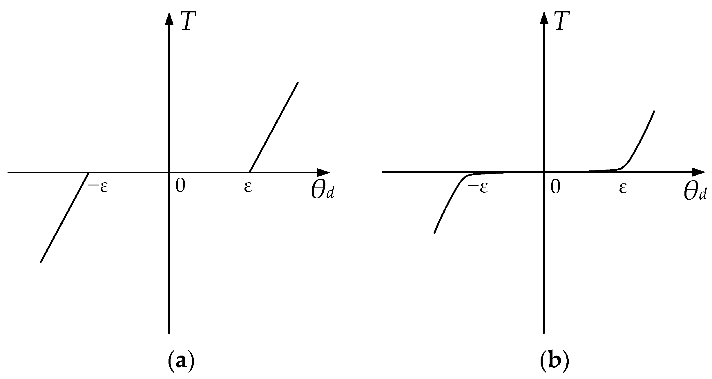
The rotary vector reducer, ball screws, and other traditional connections of the servo system are often accompanied by a nonlinear gap, typically in the form of a certain amount of clearance, with the aim of ensuring the transmission of flexibility to avoid jamming. However, the long-term operation of machinery and equipment, coupled with the inevitable effects of wear and tear, will also result in an increase in the gap. The introduction of the gap will further exacerbate the mechanical resonance. With regard to the study of clearance, the current prevailing approach is the approximate dead zone model and the dead zone model [14], as illustrated in Figure 1a,b. While the former model, despite its greater accuracy, is relatively complex and has a limited impact on the primary calculation interval, this paper establishes a dead zone model for study.

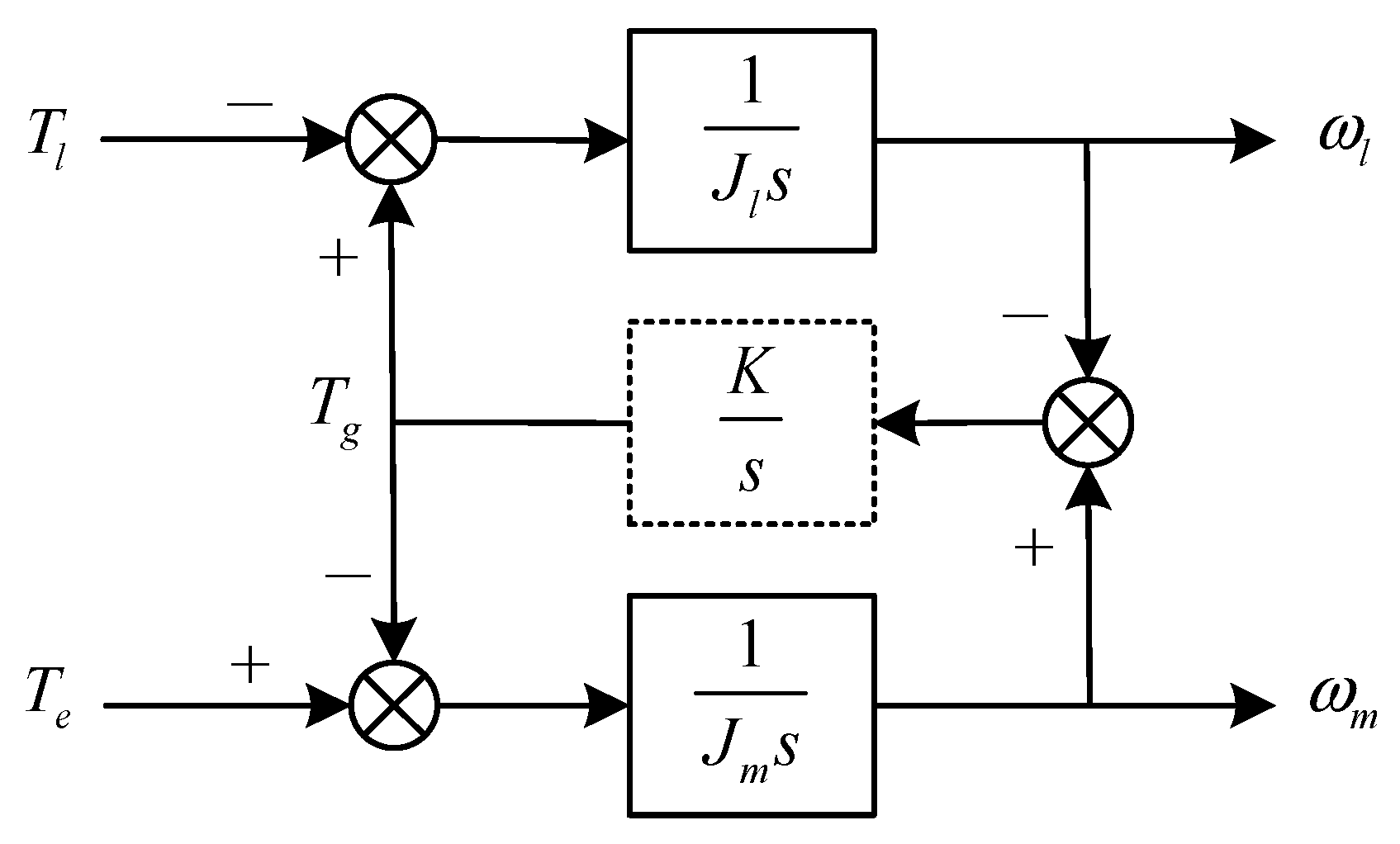
Thus, as Figure 2 shows, in a dual-inertia system, the drive motor and the load are connected via a driveshaft with a torsional stiffness of K, a damping coefficient of c, a clearance of 2ε, and a simplified ratio of 1. In this regard, Wang et al. proposed a block diagram of an equivalent model for a dual-inertia system [12].

Consider that the effect of the gap is mainly reflected in the initial position of non-engagement or changes in the direction of motion to produce positioning errors, while in the identification of mechanical parameters can be maintained in one direction of rotation, necessarily engaged. Therefore, the clearance only has an effect at the initial stage of identification and does not affect the final iteration results. Neglecting the gap, the coupling inertia and the damping coefficient of each part—that is, the mechanical parameters to be identified—are simplified as the drive motor inertia J_m, the coupling stiffness K, and load inertia J_l, and the motion process of each inertial body in the double-inertia system are analyzed to establish a mathematical model: when the drive is given a current to generate the electromagnetic torque T_e, which drives the drive motor with rotational inertia of J_m to rotate; the load side is static due to the inertia; and there is an angular difference, it causes the drive shaft to twist and deform, generating transfer torque. This torque is both the load torque of the drive motor and the driving torque of the load, which acts together with the load-side torque T_l to determine the load speed. The mathematical model of the above process is as follows:

$$\left\{\begin{array}{l}{J}_m{\ddot{\theta }}_m=T_e-T_g\hfill \\ J_l{\ddot{\theta }}_l=T_g-T_l\hfill \\ {\omega }_m={\dot{\theta }}_m\hfill \\ \begin{array}{l}{\omega }_l={\dot{\theta }}_l\hfill \\ T_g=K\left({\theta }_m-{\theta }_l\right)\hfill \end{array}\hfill \end{array}\right.$$

(1)

A simplified block diagram of the dual-inertia system is shown in Figure 3 [14].

From the diagram above, A(s) and B(s) are the transfer function; the transfer equation can be defined as

$$G_l(s)={\displaystyle \frac{{\omega }_m(s)}{T(s)}}={\displaystyle \frac{B(s)}{A(s)}}$$

(2)

In Equation (2), T(s) represents electromagnetic torque and G_l(s) represents the relationship between electromagnetic speed and electromechanical torque.

The A(s) and B(s) in the equation is

$$\left\{\begin{array}{l}A(s)=J_m{J}_l{s}^3+(J_{m}K+J_{l}K)s\hfill \\ B(s)=(J_l{s}^2+K)T_e(s)-K{T}_l(s)\hfill \end{array}\right.$$

(3)

The motor speed is determined by the electromagnetic torque and load torque together, and its transfer function is

$${\omega }_m(s)={\displaystyle \frac{(J_l{s}^2+K)}{J_m{J}_l{s}^3+(J_{m}K+J_{l}K)s}}{T}_e(s)-{\displaystyle \frac{K}{J_m{J}_l{s}^3+(J_{m}K+J_{l}K)s}}{T}_l(s)$$

(4)

where the transfer function from motor speed to electromagnetic torque is

$${\omega }_m(s)={\displaystyle \frac{(J_l{s}^2+K)}{J_m{J}_l{s}^3+(J_{m}K+J_{l}K)s}}{T}_e(s)$$

(5)

From (5), the system exhibits a pair of conjugate zero poles; the conjugate zero point is the anti-resonance frequency (ARF); the conjugate poles are the natural torsional frequency (NTF); the zero poles make the system produce a relatively strong response to the input of a specific frequency, i.e., trigger mechanical resonance.

$${\omega }_{\mathrm{ARF}}=\sqrt{{\displaystyle \frac{K}{J_l}}}$$

(6)

$${\omega }_{\mathrm{NTF}}=\sqrt{{\displaystyle \frac{J_{m}K+J_{l}K}{J_m{J}_l}}}$$

(7)

3. Identification of Mechanical Parameters for Dual-Inertia Systems

3.1. The Principle of Least Squares

The least square (LS) method was first introduced by K.F. Gauss in his work on the prediction of celestial orbits and is based on the principle of minimizing the sum of the squares of the errors in each set of data. In 2013, Seppo E. S.’s team at Aalto University, Finland combined the least squares method to derive the parameters in the discrete domain and then transformed them to the frequency domain by the zero-pole matching method to obtain the identification results [8]. In this article, the n sets of input and output observations of an observable system are expressed as in (8), and the estimates of the system parameters can be obtained according to the least squares method as in (9).

$$\{y(k),u(k),k=1,2,\cdots ,n\}$$

(8)

$$\mathit{\theta }={({\mathit{\varphi }}^{\mathrm{{\rm T}}}\mathit{\varphi })}^{-1}{\mathit{\varphi }}^{\mathrm{{\rm T}}}\mathit{Y}$$

(9)

where θ is the estimate output of system, ϕ is the data vector matrix, and Y is the system output matrix.

However, when using LS, every time an observation is added, it is necessary to re-solve the identification of the new observation together with all the previous data, which leads to a large number of repeated calculations, and the quantity of data increases dramatically over time, which seriously affects the computational speed of the system. In order to improve computational efficiency, the recursive least square (RLS) algorithm is introduced, which is based on the idea of assuming that the deviation of the estimated values of the system parameters at k moments and k – 1 moments is ∆, i.e.,:

$$\mathit{\theta }(k)=\mathit{\theta }(k-1)+\mathrm{\Delta }$$

(10)

Also, by the least square’s method, the estimate for moment k is obtained as

$$\mathit{\theta }(k)={[{\mathit{\varphi }}^T(k)\mathit{\varphi }(k)]}^{-1}{\mathit{\varphi }}^T(k)\mathit{Y}(k)$$

(11)

in which $\mathit{\varphi }(k)=\left(\begin{array}{c}\mathit{\varphi }(k-1)\\ {\mathit{\phi }}^T(k)\end{array}\right),\mathit{Y}(k)=\left(\begin{array}{c}\mathit{Y}(k-1)\\ y(k)\end{array}\right)$.

Let the covariance matrix P(k) be

$$\mathit{P}(k)={[{\mathit{P}}^{-1}(k-1)+\mathit{\phi }(k){\mathit{\phi }}^T(k)]}^{-1}$$

(12)

Thus:

$${\mathit{P}}^{-1}(k)={\mathit{P}}^{-1}(k-1)+\mathit{\phi }(k){\mathit{\phi }}^T(k)$$

(13)

From (11) and (12), the estimate for the k – 1 moment is

$$\mathit{\theta }(k-1)=\mathit{P}(k-1){\mathit{\varphi }}^T(k-1)\mathit{Y}(k-1)$$

(14)

From (13) and (14):

$${\mathit{\varphi }}^T(k-1)\mathit{Y}(k-1)=[{\mathit{P}}^{-1}(k)-\mathit{\phi }(k){\mathit{\phi }}^T(k)]\mathit{\theta }(k-1)$$

(15)

Thus, the estimates of the system parameters at moment k can be corrected by moment k – 1 to obtain

$$\mathit{\theta }(k)=\mathit{P}(k){\mathit{\varphi }}^{{\rm T}}(k)\mathit{Y}(k)=\mathit{\theta }(k-1)+\mathit{K}(k)[y(k)-{\mathit{\phi }}^T(k)\mathit{\theta }(k-1)]$$

(16)

where K(k) the gain vector and K(k) = P(k) φ(k).

The iterative formula for the recursive least square’s method can be obtained from the matrix inverse lemma as well as (15) as

$$\left\{\begin{array}{c}\mathit{\theta }(k)=\mathit{\theta }(k-1)+\mathit{K}(k)[y(k)-{\mathit{\phi }}^T(k)\mathit{\theta }(k-1)] \hfill \\ \mathit{P}(k)=[\mathit{E}-\mathit{K}(k){\mathit{\phi }}^T(k)]\mathit{P}(k-1)\hfill \\ \mathit{K}(k)=\mathit{P}(k-1)\mathit{\phi }(k)/[1+{\mathit{\phi }}^T(k)\mathit{P}(k-1)\mathit{\phi }(k)]\hfill \end{array}\right.$$

(17)

where I is the unit matrix. Although the RLS algorithm solves the problem of a large number of repeated calculations well, its default is that the old and new data are equally important, which will not reflect the real-time status of the motor. Therefore, the attenuation coefficient is added to RLS to weaken the influence of the old data on the discriminated values, forming the recursive least squares method with forgetting factor, and the iteration formula is modified as

$$\left\{\begin{array}{c}\mathit{\theta }(k)=\mathit{\theta }(k-1)+\mathit{K}(k)[y(k)-{\mathit{\phi }}^T(k)\mathit{\theta }(k-1)]\hfill \\ \mathit{P}(k)={\displaystyle \frac{1}{\lambda }}[\mathit{E}-\mathit{K}(k){\mathit{\phi }}^T(k)]\mathit{P}(k-1)\hfill \\ \mathit{K}(k)=\mathit{P}(k-1)\mathit{\phi }(k)/[\lambda +{\mathit{\phi }}^T(k)\mathit{P}(k-1)\mathit{\phi }(k)]\hfill \end{array}\right.$$

(18)

In the formula, the value range of forgetting factor λ is usually 0.9~1. The smaller λ is, the faster the convergence speed is, the larger λ is, and the smaller the fluctuation in algorithm recognition results is. After many simulations and experimental verification, λ = 0.99 was finally selected for this topic.

3.2. Mechanical Parameter Identification Algorithm for Dual-Inertia Systems

In order to apply FFRLS, the system transfer function needs to be converted from the frequency domain to the discrete domain. The commonly used discretization methods [15] and their advantages and disadvantages are listed below:

(1)

First-order backward difference: the mapping relationship is severely distorted, the transformation accuracy is low, and there are fewer engineering applications;

(2)

First-order forward difference: the mapping relationship is severely distorted, and the stability of the system after discretization cannot be guaranteed (unless the sampling period is small);

(3)

Bilinear transformation (Tustin) method: better accuracy, easy to apply, the disadvantage is that the high-frequency characteristics of the distortion are serious;

(4)

Zero-pole matching method: due to the need to decompose the transfer function into zero-pole form and the need for steady-state gain matching, the application is not convenient enough;

(5)

z-conversion method (impulse response invariant method): z-conversion is more cumbersome and prone to frequency aliasing;

(6)

z-transform method with keeper: also has the disadvantages of z-transform.

Considering the frequency range of the dual-inertia system and the ease of application of the discrete method, Tustin’s method is used in this topic. T_s is the discrete sampling period; the transfer function of the system in the discrete domain is obtained as

$$s=(2/T)(1-z^{-1})/(1+z^{-1})$$

(19)

$${\omega }_m(z)={\displaystyle \frac{{\theta }_1{z}^3+{\theta }_2{z}^2+{\theta }_{2}z+{\theta }_1}{z^3+{\theta }_3{z}^2-{\theta }_{3}z-1}}{T}_e(z)-{\displaystyle \frac{{\theta }_4{z}^3+3{\theta }_4{z}^2+3{\theta }_{4}z+{\theta }_4}{z^3+{\theta }_3{z}^2-{\theta }_{3}z-1}}{T}_l(z)$$

(20)

Among the above equation:

$$\left\{\begin{array}{c}{\theta }_1={\displaystyle \frac{4J_l{T}_s+K{T_s}^3}{8J_m{J}_l+2(J_{m}K+J_{l}K){T_s}^2}}\hfill \\ {\theta }_2={\displaystyle \frac{-4J_l{T}_s+3K{T_s}^3}{8J_m{J}_l+2(J_{m}K+J_{l}K){T_s}^2}}\hfill \\ {\theta }_3={\displaystyle \frac{-24J_m{J}_l+2(J_{m}K+J_{l}K){T_s}^2}{8J_m{J}_l+2(J_{m}K+J_{l}K){T_s}^2}}\hfill \\ {\theta }_4={\displaystyle \frac{K{T_s}^3}{8J_m{J}_l+2(J_{m}K+J_{l}K){T_s}^2}}\hfill \end{array}\right.$$

(21)

Convert the above equation into the expression required by FFRLS, and the output ω_m(k) at k stage is

$$\begin{array}{ll}\hfill {\omega }_m(k)=& {\theta }_1[T_e(k)+T_e(k-3)]+{\theta }_2[T_e(k-1)+T_e(k-2)]\hfill \\ & +{\theta }_3[{\omega }_m(k-2)-{\omega }_m(k-1)]+{\omega }_m(k-3)\hfill \\ & -{\theta }_4[T_l(k)+3T_l(k-1)+3T_l(k-2)+T_l(k-3)]\hfill \end{array}$$

(22)

Let the output be a parameter vector and a data vector as follows:

$$\begin{array}{ll}\hfill \mathit{\theta }=& {[{\theta }_1 {\theta }_2 {\theta }_3 1 {\theta }_4]}^{\mathrm{T}}\hfill \\ \hfill \mathit{\varphi }=& [T_e(k)+T_e(k-3),T_e(k-1)+T_e(k-2),\hfill \\ & -{\omega }_m(k-1)+{\omega }_m(k-2),{\omega }_m(k-3),\hfill \\ & -(T_l(k)+3T_l(k-1)+3T_l(k-2)+T_l(k-3)){]}^{\mathrm{T}}\hfill \end{array}$$

(23)

The data vector consists of the sampled values of electromagnetic torque T_e, load torque T_l, and motor speed ω_m, and the initial values are all set to 0. The parameter vector corresponds to five system parameters, of which the coefficient of ω_m(k – 3) is always 1 and does not need to be identified; here, all the initial values of the parameters are still set to 0.01 according to empirical formulas, the final results of which can be used to judge whether the identification algorithm can converge to the true value or not; the initial value of the covariance matrix P (0) = 10⁶ I(6). According to the initial value and the input and output, the results of parameter identification in the discrete domain are calculated iteratively by (19).

After the discrete domain parameter identification is completed, the equation is solved by substituting into (21) to complete the conversion of the parameters to be sought from the discrete domain to the frequency domain. The equations are solved as (24), which are all polynomials, avoiding the nonlinear operations such as ln function brought by other discrete methods, saving computational resources and parameter conversion time. It is worth noting that there are four equations and three to-be-sought mechanical parameters in (21), among which θ₄ does not need to participate in the conversion process, which means that the load torque T_l only participates in the iteration as a compensating effect without affecting the conversion process.

$$\left\{\begin{array}{c}{J}_m=-{\displaystyle \frac{T_s({\theta }_3-1)}{6{\theta }_1-2{\theta }_2}}\hfill \\ J_l={\displaystyle \frac{2T_s(2{\theta }_1-{\theta }_2+{\theta }_1{\theta }_3)}{(3{\theta }_1-{\theta }_2\left)\right({\theta }_1+{\theta }_2)}}\hfill \\ K={\displaystyle \frac{16{\theta }_1-8{\theta }_2+8{\theta }_1{\theta }_3}{T_s{(3{\theta }_1-{\theta }_2)}^2}} \hfill \end{array}\right.$$

(24)

The flowchart of the system identification procedure is shown in Figure 4.

4. Simulation Verification

Algorithmic Validity

Least squares with forget factor, also known as exponentially weighted least squares or recursive least squares with a forget factor, is an adaptive algorithm used for online parameter estimation in time-varying systems. In order to verify the effectiveness of the above algorithm, the model as Figure 5 shown is built and simulated in MATLAB 2023b/Simulink, and the model parameters are consistent with the experimental platform, as shown in

Table 1. Main parameters of the motor.

Parameters	Value
Rated power (W)	750
Rated current (A)	3
Rated torque (N·m)	2.39
Poles	5
Inertia (kg·m2)	1.82 × 10−4

.

Plum blossom coupling is used as the flexible coupling, and since its stiffness is unknown, chirp sweep method is used to determine the resonance characteristics of the system and determine the coupling stiffness, which is used to compare with the identified results. Given the d-axis current i_d* = 0 and q-axis current i_q* = sin (2π(125 t²)), the motor speed response waveform is shown in Figure 6, and its FFT analyze result is shown in Figure 7. The anti-resonance frequency is 204.8 Hz; according to Equation (4), the stiffness of the coupling can be calculated as K = 301.36 N·m/rad.

The rotational speed reference signal is n_r* = 200 + 200 sin (5πt) rpm, the simulation sampling period is 0.0001 s, and the identification results are shown in Figure 8 and Figure 9.

The discrete domain parameter θ(4) converges from the initial value of 0.01 to the true value of 1 in (23), indicating the effectiveness of the current parameter identification algorithm. The comparison of the identification results with the actual values is shown in

Table 2. Simulation results of mechanical parameter identification of dual-inertia system.

Parameters	Ture Value	Identification Value	Identification Error (%)
Jm (kg·m2)	1.82 × 10−4	1.813 × 10−4	0.38
Jl (kg·m2)	1.82 × 10−4	1.828 × 10−4	0.44
K (N·m/rad)	301.36	301.7	0.11

, with small identification errors and high identification accuracy.

5. Influence of System Parameters on Recognition Accuracy

(1)

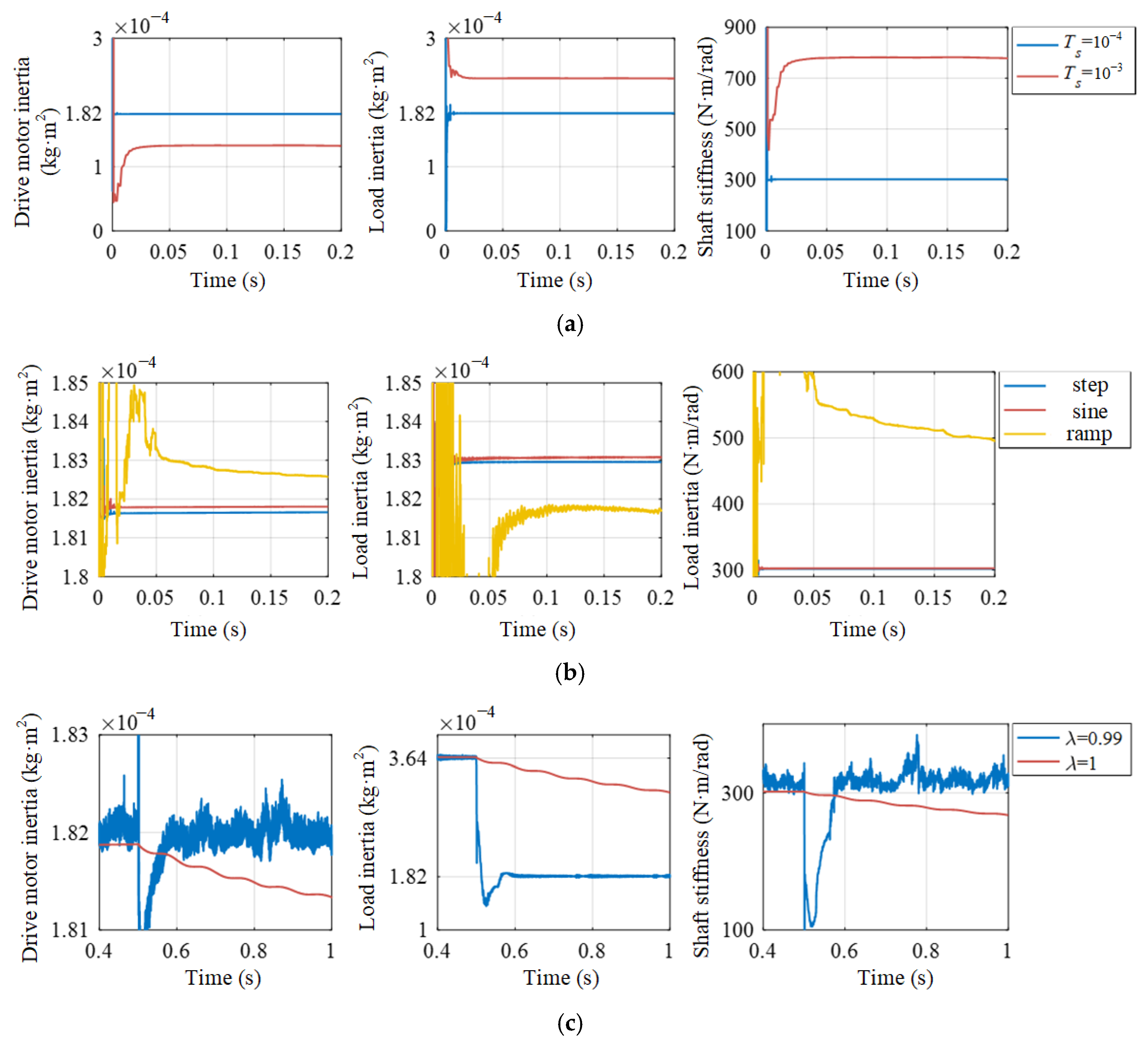
Discrete time

Yang, M. et al. point out that the smaller the discretization period is, the closer the discrete domain function is to the continuous domain function, and the higher the discrimination accuracy is [16]. In order to correspond to the experiment platform hardware, we choose the switching frequency between 1 k~10 kHz. Figure 10a gives a comparison of the identification results in two cases where T_s is 0.001 s and 0.0001 s, respectively. The convergence process of the recognition algorithm is slow when the discrete period is large. The numerical accuracy of the final convergence is also poor.

(2)

Given signal

Given different speed signals, the comparison of the recognition results is shown in

Table 3. Parameter identification results for different given speeds.

No.	Given Type	Value (rpm)	Jm Identification Error (%)	Jl Identification Error (%)	K Identification Error (%)
1	Step	50	0.05	0.53	0.44
2		200	0.29	0.44	0.59
3	Ramp	1000 t	0.38	0.06	40.3
4		4000 t	0.42	0.20	6.85
5	Sine	200 sin (5πt)	0.05	0.57	0.46
6		200 sin (10πt)	0.16	0.37	0.49

. Under the three signal forms, the recognition accuracies of the inertia J_m and J_l on both sides are high and can reach within 1% under ideal simulation conditions. However, the identification error of the shaft stiffness K under the slope given speed signal is extremely high, as high as 40.3%. As the slope of the given signal increases, the identification error decreases significantly. The simulation waveforms are shown in Figure 10b for the second, fourth, and sixth given signals. The convergence speeds and recognition accuracies of the step signal and sinusoidal signal do not differ much, but the convergence speeds are relatively slow, and the recognition results fluctuate a lot in the slope of the given signal. From the derivation of the algorithm, it can be seen that the recognition process depends on the transient process of the motor speed rise, while the acceleration is small and the transient process is short when the ramp is given, which is not conducive to the recognition.

(3)

Forgetting factor

As mentioned before, the forgetting factor λ affects the convergence speed and volatility of the identification results. In the real working condition, the weapon station will have the situation of sudden unloading, which leads to the sudden change in inertia on the load side. Therefore, relevant experiments are needed to verify the robustness of the algorithm. Figure 10c shows the recognition waveforms under different forgetting factors when the load inertia is suddenly reduced at 0.5 s. When λ = 1, the convergence is still not possible within 0.5 s, and the convergence speed is slow, but the waveform of the recognition result is smoother; when λ = 0.99, the recognition result is re-converged to the vicinity of the true value within 0.1 s, and the convergence speed is fast, but there are many signal burrs and fluctuation is large.

After comprehensive consideration, in the mechanical parameter identification experiment, this paper selected a sinusoidal signal as the given signal, with forgetting factor λ = 0.99. Discretization time needs to be based on the performance of the controller and other algorithms to further determine the time required.

6. Experimental Verification

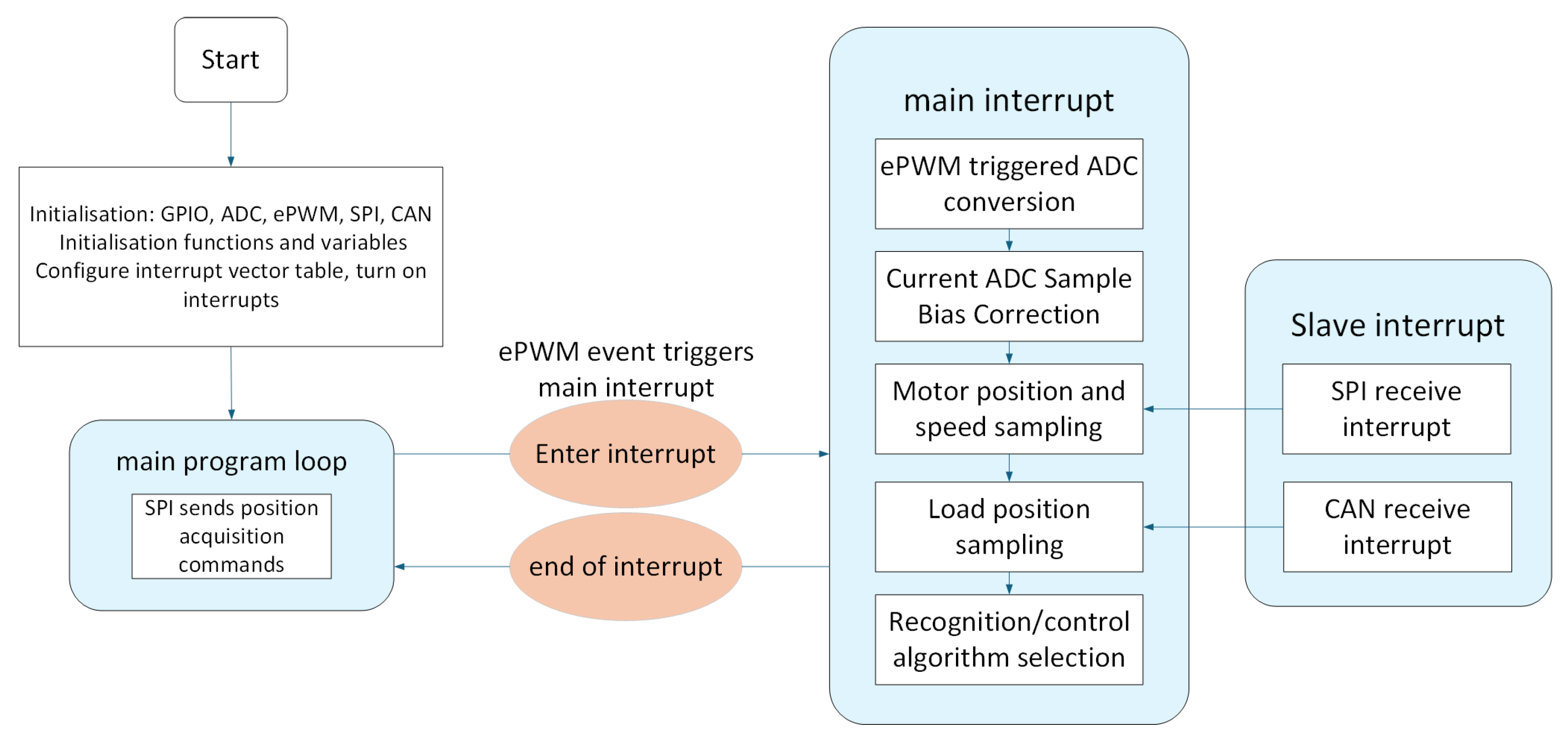
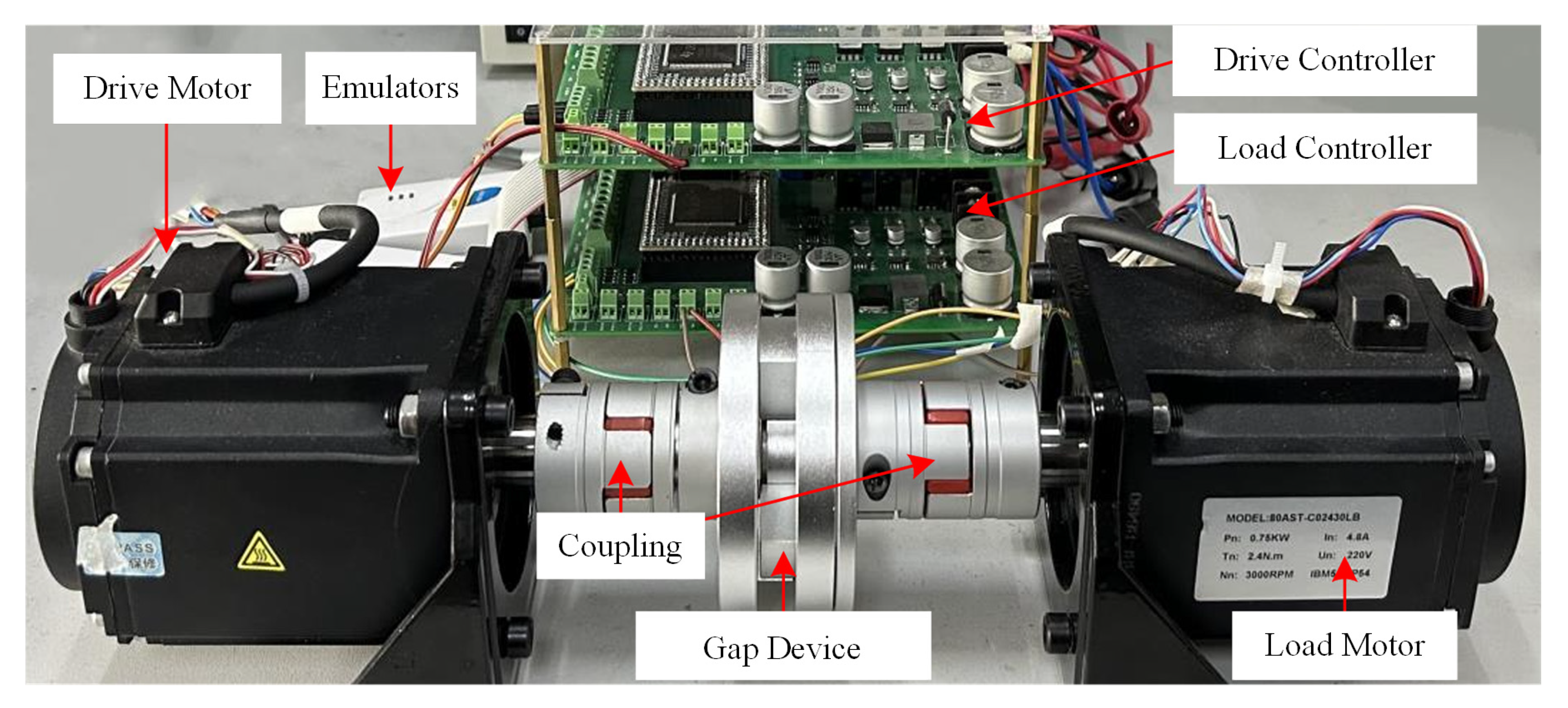
Details on the experimental platform of this research’s software platform and hardware platform are shown in Figure 11 and Figure 12.

The controller of the experimental platform uses the DSP TMS320F28335 chip from Texas Instruments (Dallas, TX, USA). The three-phase currents of the motor are obtained through the sampling module. Through the real-time position feedback from the 18 bits AS5047P absolute encoder, the ePWM output duty cycle is calculated and updated to drive the motor rotation. The load-side controller is the same as that of the drive-side, and both transmit position signals in both directions via CAN communication. The experimental platform uses two M02430LBX motors.

The parameters of the platform are shown in

Table 4. Dual-inertia system experimental platform parameters.

Parameters	Values
Switching frequency (Hz)	10 k
Rated power (W)	750
Rated current (A)	2
Rated rotation speed (rpm)	3000
Rotor inertia (kg·m2)	1.82 × 10−4
ADC resolution	12 bits
DAC resolution	12 bits

below.

The iterative algorithm is a fifth-order matrix operation, which takes more time, and FFRLS also has requirements for discrete time (i.e., sampling time), so it is necessary to test the algorithm time. The clock period of the controller used in the experiment is 0.67 ns, and the running time of the test programmed using breakpoints is 4994 clock cycles (33 μs) for the motor control programmed. The time of the parameter recognition algorithm is shown in

Table 5. Dual-inertia system parameter identification time test.

Load Condition	Order of Operation	Iteration Duration	Conversion Time	Total Duration
Unladen	4	46 μs	5 μs	51 μs
Payload	5	84 μs	4 μs	88 μs

, with a total running time of 84 μs for no-load operation, and 121 μs for with-load operation. When the current loop control frequency is 10 kHz and the speed loop control frequency is 1 kHz, the recognition time in the loaded case the discrimination time exceeds one current loop cycle. In order to simplify the control and improve the recognition accuracy as much as possible, the sampling time is 0.0002 s.

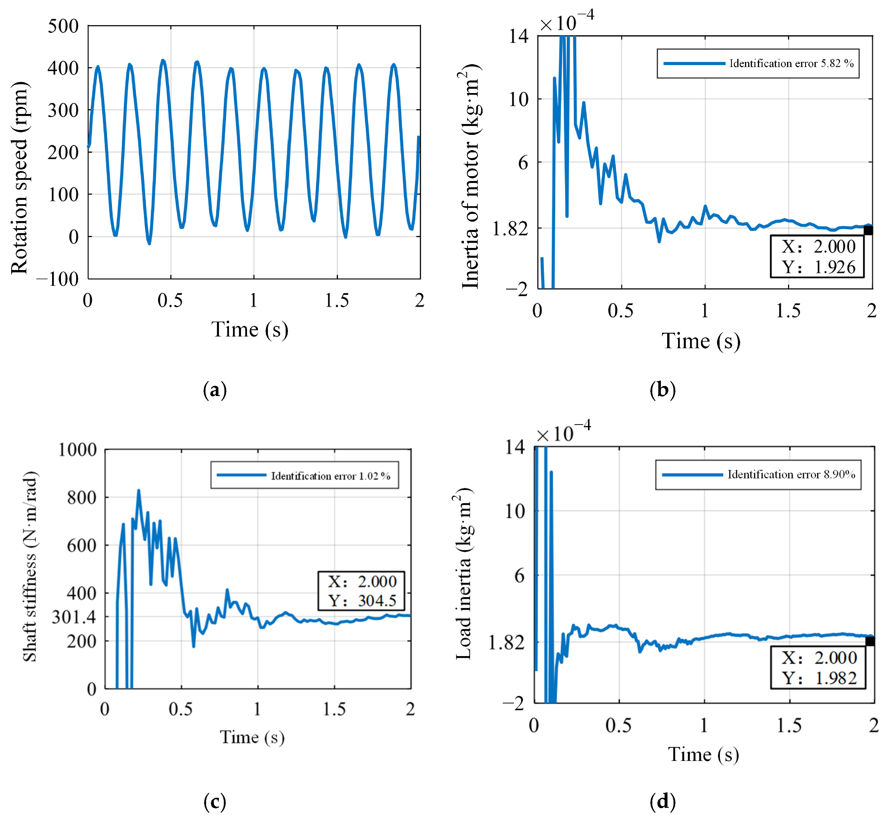
Given n_r* = 200 + 200 sin (5πt) rpm with sinusoidal speed, the system response waveform and the convergence waveform of the discriminated values of mechanical parameters are shown in Figure 13. It is considered to be basically converged in 0.6 s, and the discriminated values of the drive motor inertia, load inertia, and shaft stiffness in 2 s are 1.93 × 10⁻⁴ kg·m², 1.98 × 10⁻⁴ kg·m², and 304.5 N·m/rad, with identification errors of 5.82%, 8.90%, and 1.02%, respectively.

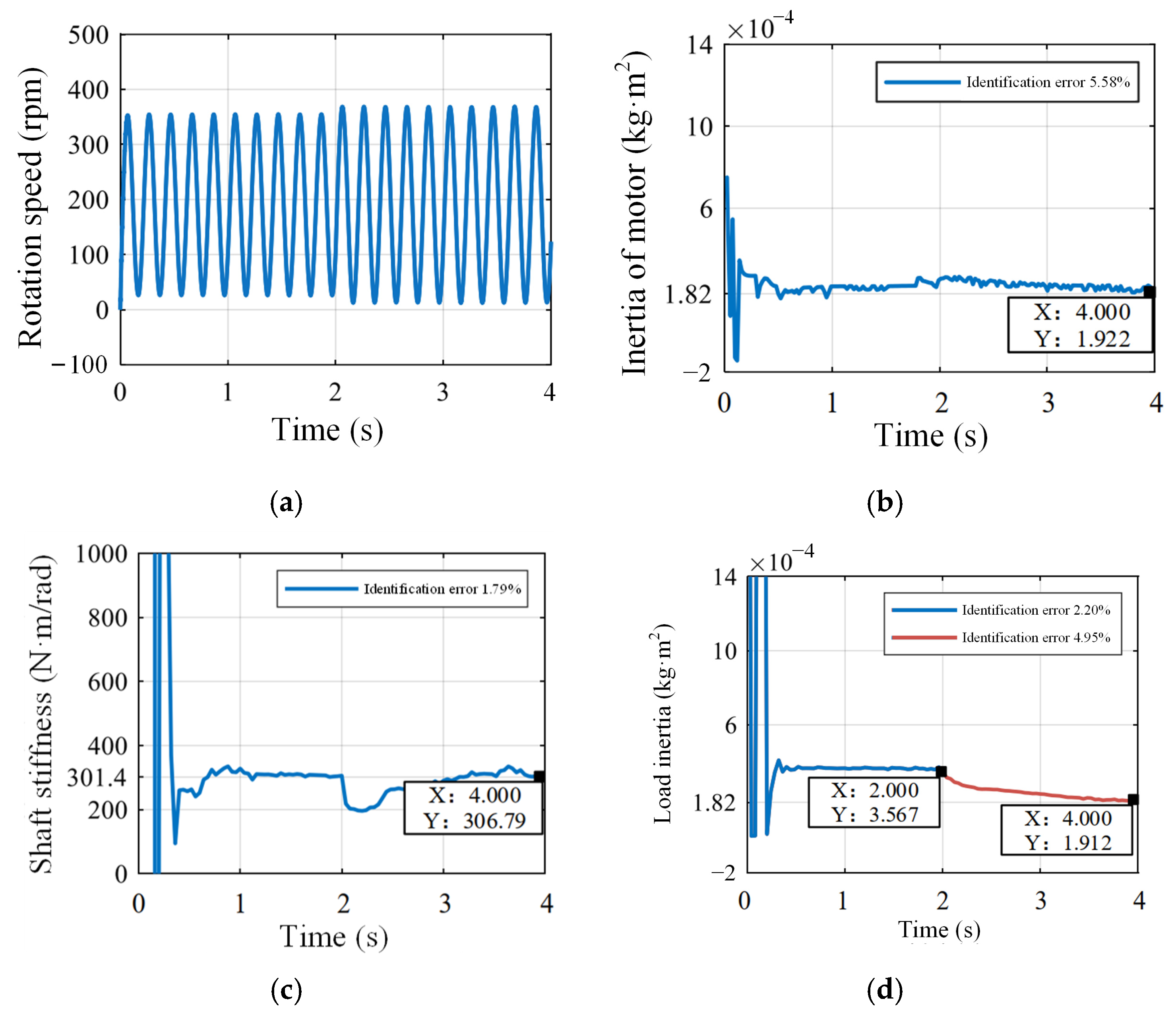
Figure 14 shows the system response and recognition waveforms when the load inertia changes suddenly. The load inertia decreases from 2 J_l to J_l at 2 s, the drive motor inertia and shaft stiffness converge to the real value after fluctuation, while the load inertia converges slower and the recognition accuracy decreases from 2.2% to 4.95%, which is due to the fact that the covariance matrix P is not re-initialized.

The experiment shows that the mechanical parameter identification algorithm of the dual-inertia system can simultaneously identify three main mechanical parameters online. From the experiment results shown in Figure 13 and Figure 14, all the identification errors are less than 10%, which shows the algorithm has high identification accuracy and certain robustness.

7. Conclusions

In this paper, a new algorithm is constructed and validated using recursive least squares with forgetting factor for the problem of identifying the mechanical parameters of a two-inertia elastic system. First, the dual-inertia system is modeled and analyzed to obtain its mathematical model. Second, using the recursive least squares method with forgetting factor, an online identification algorithm for the main mechanical parameters of the dual-inertia system is constructed, and the drive motor inertia, load inertia, and coupling stiffness of the system are accurately obtained. This backstepping adaptive controller based on backtracking compensation can effectively compensate for the backtracking effect, improve the stability of the system, and realize accurate tracking. Finally, the algorithm is simulated and experimentally verified. The experimental results show that the algorithm can recognize the three main mechanical parameters at the same time, with high recognition accuracy and a certain robustness. However, when the system structure is unknown (single inertia, thrip inertia, and above), the identification algorithm cannot be implemented, making it necessary to conduct research on systematization and generalization algorithms in a nonlinear system.