A Hybrid Dual-Axis Solar Tracking System: Combining Light-Sensing and Time-Based GPS for Optimal Energy Efficiency

Abstract

Fixed solar panels face significant energy loss as they cannot consistently capture optimal sunlight. Because of that, the overall efficiency of the PV panel will be reduced, and the installation requires larger land space to generate appropriate power; this stems from the use of a dual-axis solar tracking system, which can significantly increase overall energy production. The system is based on the combination of two approaches to precisely track the sunlight: first, using multiple LDRs (light-dependent resistors) as photo sensors to track the position of the sun by balancing the resistivity using a proportional integral deprival (PID) controller, and the second approach using the time-based control for cloudy days when sunlight is diffused, getting the time GPS coordinates and time to calculate the accurate position of the sun by determining the azimuth and altitude angle. This dual system significantly improves energy production by 33.23% compared to fixed systems and eliminates errors during shaded conditions while reducing unnecessary energy use from continuous GPS activation. The prototype uses two linear actuators for both angles and a 100-watt solar panel mounted on the dual-axis platform.

1. Introduction

In recent years, as industries and technologies advances, the world’s energy needs have grown continuously. The process of extracting and using conventional energy sources releases greenhouse gases, which play a major role in the phenomenon of global warming, a pressing global concern [1]. One type of renewable and sustainable energy that may serve as an effective substitute for traditional primary energy sources is solar energy [2]. In some developed countries, the cost of photovoltaic (PV)-based energy generation has already reached parity with fossil-fuel-based energy resources, making it a viable and competitive alternative [3,4]. Straightforward installation, low maintenance requirements, and the ease of moving components are the leading causes behind the faster growth of solar energy compared to any other solar collecting technique. This growth is reflected in the overall increase in solar energy capacity and utilization, which amounts to 29.6% [5]. A solar cell, which is referred to as a photovoltaic (PV) cell, is any device that uses its photovoltaic action concept to transform solar radiation into DC current. The advancement of alternative sources of energy has drawn global interest from academics due to numerous investigations demonstrating that renewable sources of energy are more sustainable and friendly to the environment than fossil fuels [6,7,8,9]. While “photovoltaic cell” is a term often used in technical contexts, “solar cell” is more commonly used when referring to equipment specifically designed to absorb solar energy [10].

The solar spectrum varies depending on the precise moment of day and position, impacting the performance of PV systems. South-facing tilted PV arrays achieve a tracking efficiency of 95% around noon compared to continuous tracking systems, and dual-axis tracking can increase annual output by up to 36% [11]. Per-day energy generation sees a 25% increase with single-axis tracking and a 35% increase with dual-axis tracking compared to fixed PV modules [12]. Therefore, designing a model that combines dual-axis solar tracking with light-dependent resistor (LDR) sensors or global positioning system (GPS) technology can significantly improve PV energy generation and motion tracking efficiency. This implementation will result in a system with higher tracking efficiency than fixed flat-plate approaches while utilizing sensors that are less expensive than conventional options [13]. The solar spectrum varies depending on the precise moment of day and position. Due to the sun’s continuous motion throughout the daytime, a fixed PV panel inclined at the ideal tilt angle is inadequate [14].

Photovoltaic panels are considered the most advanced renewable energy source for increasing the energy output of solar systems and generating electricity, leading to the implementation of sun-tracking and panel position adjustment systems. The sunbeam frequently changes direction seasonally, causing low efficiency in current solar conversion systems. The sun’s rays coordinate themselves in two orientations relative to Earth: moving along its radiation axis and the horizon. The first is the daily east–west flow, where the angle of incidence varies as the sun moves. A dual-axis solar tracker can increase output power by allowing flexible motion of the solar panel around both the vertical and horizontal axes. With this technology, the sun is tracked effectively, and the solar panel provides maximum energy. Variations in the sun’s azimuth angle and the Earth’s elevation (zenith angle) necessitate solar trackers to have two degrees of freedom to continually monitor the sun [15,16].

Single-axis tracking and dual-axis tracking are the two main categories of solar tracking systems. Dual-axis tracking ensures that the tracked panel always receives the maximum possible solar energy due to its two rotatable axes. It is determined that, with 54.39% of the papers consulted, the closed-loop solar tracking control approach is the most utilized. The most used control algorithms in active solar tracking systems are on–off (57.02%), fuzzy logic (10.53%), proportional–integral–derivative (6.14%), and proportional–integral (4.39%) [17].

When a PV module is implemented, its movement about the rotation axis can be predicted using a set of photovoltaic (PV) or light-dependent resistor (LDR) sensors and fixed time-based measurements using GPS for latitude and time. The system’s control unit includes a microcontroller, a sensor unit, an actuator motor, and a power supply. Linear actuator control drives are activated by signals gathered by the sensors to follow the sun and maintain the panel’s normal direction of irradiation [18].

To harness the maximum power from solar panels, tracking the solar beam throughout the day is crucial, as it can exponentially increase the panels’ efficiency. Various solar tracking techniques and methods, such as biphasic liquid tanks and single-axis and dual-axis systems, fall under two main categories: passive and active solar tracking systems [19].

The passive solar tracking system works on the principle of heat conversion using liquid in two different tanks to track the sun. In contrast, the active solar tracking system uses transducers and actuators to follow the solar pattern. Depending on the system’s degrees of freedom, there are two main types of active solar tracking systems: single-axis and dual-axis [20].

Active solar tracking technology can increase the precision of solar tracking by using a motor or hydraulic actuator managed by a group of controller units to tilt the solar panel according to the sun’s movement. Sun-pointing sensors are typically used in solar tracking models to enhance the power-collecting capacity for PV installations. When the sun’s radiation strikes perpendicular to the panels’ surface, the solar power system generates more electrical power. The system’s complexity depends on the number of axes involved in moving the solar panels horizontally, vertically, or both. Single-axis tracking models are less complex and more affordable than dual-axis tracking models, but the latter outperforms the former in efficiency.

Despite the development of numerous solar tracking technologies, efficiency and power output remain challenges [21]. Installing PV panels on solar tracking systems increases solar radiation exposure, thereby achieving high PV system efficiency. Tracking can be carried out manually, automatically, semi-automatically, continually, or constantly [22]. This approach is favored for its longevity, ease of installation, economic spending and maintenance costs, and higher efficiency, resulting in a lower levelized cost of energy (LCOE) [23]. However, PV energy is not without objections, as the vast tracts of land required for grid-connected PV plants typically become unusable for agri-food production [24]. According to studies, photovoltaic solar energy produced 270 TWh of power in 2022, a 26% increase over 2021. 2016 saw solar PV overcome wind and hydropower as the third-largest source of green power. To achieve the Net Zero Scenario’s objective of 8300 TWh in 2030 from the current level of 1300 TWh, a yearly average increase of 26% in energy production must be obtained between 2023 and 2030. The rate of growth is comparable to that of 2022, but perseverance will be needed as the PV market expands [9]. The

Table 1. The comparison of cost and payback time of various tracking systems.

Solar Tracking System	Cost of Installing the System per Watt	Recovery Time
Fixed solar panel	Vary from $2 to $2.4 per watt	For crystalline systems 1.5 to 3.5 years and for thin film 1 to 1.5 years.
Single-axis tracking	Around $1.17 per watt according to efficiency.	3 years for tracker investment.
Dual-axis tracking	Around $0.36 per watt according to efficiency.	3.5 to 5 years for tracker investment.

presents the total cost and payback period for different types of solar installations.

Alternative methods of increasing the efficiency of solar panels, such as passive cooling of the double junction and triple junction solar cells, can increase the efficiency up to 42.0%. There are various techniques to reduce the temperature of the cells. A few of them use an aluminum plate of 2mm thickness as a heat sink [25], using different heatsink configurations (TEG, HS, TEG-HS, and TEG-micro-channel heat pipe (MCHP)-HS) [26]. In addition to heatsinks, there are other ways to reduce the temperature, such as liquid immersion, natural ventilation, heat pipes, and using phase-change materials [27]. Although passive cooling does not require continuous power consumption, it needs a large initial budget. The best solution for getting maximum efficiency for the solar cell is to use the combination of both dual-axis solar tracking systems equipped with passive heat dissipation techniques. In one of the experiments done at the Ferdowsi University of Mashhad, Iran, they performed an experiment using a test tube filled with deionized water and silicon carbide nanofluid to achieve a power increase similar to that of a fixed-based system from 9.64 W to 20.8 W, more than double the fixed system [28].

Importance of Using This System

The efficiency of static solar panels remains a challenge, particularly in applications where space is limited and maximizing energy output is crucial. In such contexts, including cruise ships, automobiles, and buildings with restricted space, the implementation of dual-axis solar tracking systems can play a transformative role. Unlike fixed systems, dual-axis trackers adjust the position of solar panels in real time to follow the sun’s trajectory across the sky, ensuring optimal sunlight capture and significantly enhancing energy efficiency.

Therefore, the proposed system is illustrated in Figure 1. This system provides precise solar tracking, using real-time sunlight sensing and time-based tracking for cloudy weather. This system is for cruise ships, where dual-axis trackers provide a reliable renewable energy source, reducing fuel reliance and emissions. Electric and hybrid automobiles can extend driving ranges and reduce charging frequency by optimizing solar energy capture. Urban buildings with limited roof space can generate more electricity from their solar installations, sustainably meeting a more significant portion of their energy needs. This project aims to design and implement a precise dual-axis solar tracking system using real-time sensors, combining light-dependent resistors (LDRs), photodiodes, and GPS to achieve accurate sun tracking, mitigate calibration errors, and maximize solar exposure. By addressing the efficiency challenges of static solar panels, this innovative solar tracking technology has the potential to enhance sustainability and energy independence across various sectors.

2. Design Methodology

The dual-axis solar tracking system can track the sun’s movements in two-axis motion.

The linear actuators rotate the solar panel in two axes to change the direction of the solar panel. The proposed methodology combines two different solar tracking systems by combining real-time solar tracking using LDR with time-based solar prediction algorithms using GPS for latitude and time to precisely track the sun’s movement even on shady days, as illustrated in the block diagram in Figure 2.

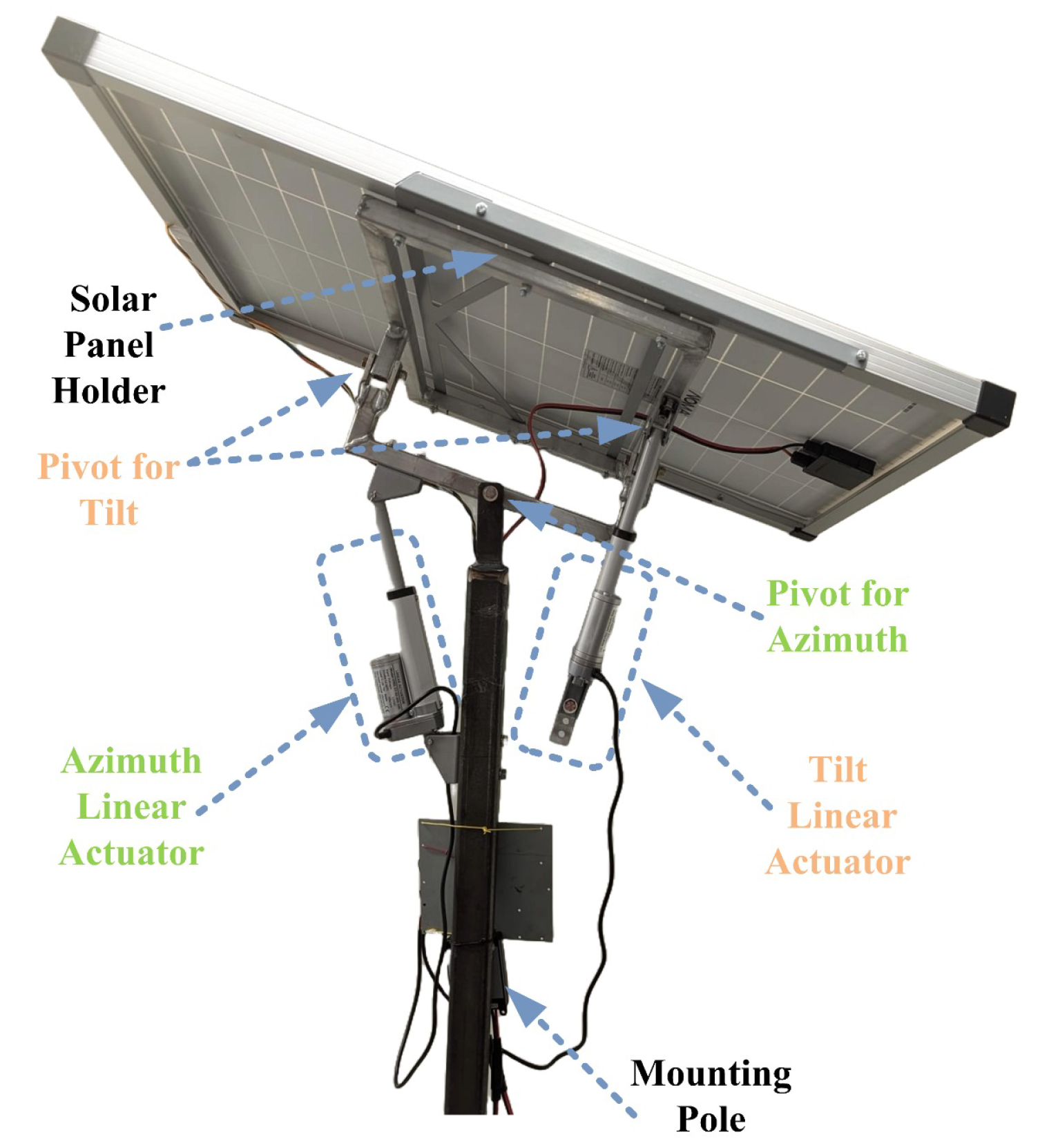
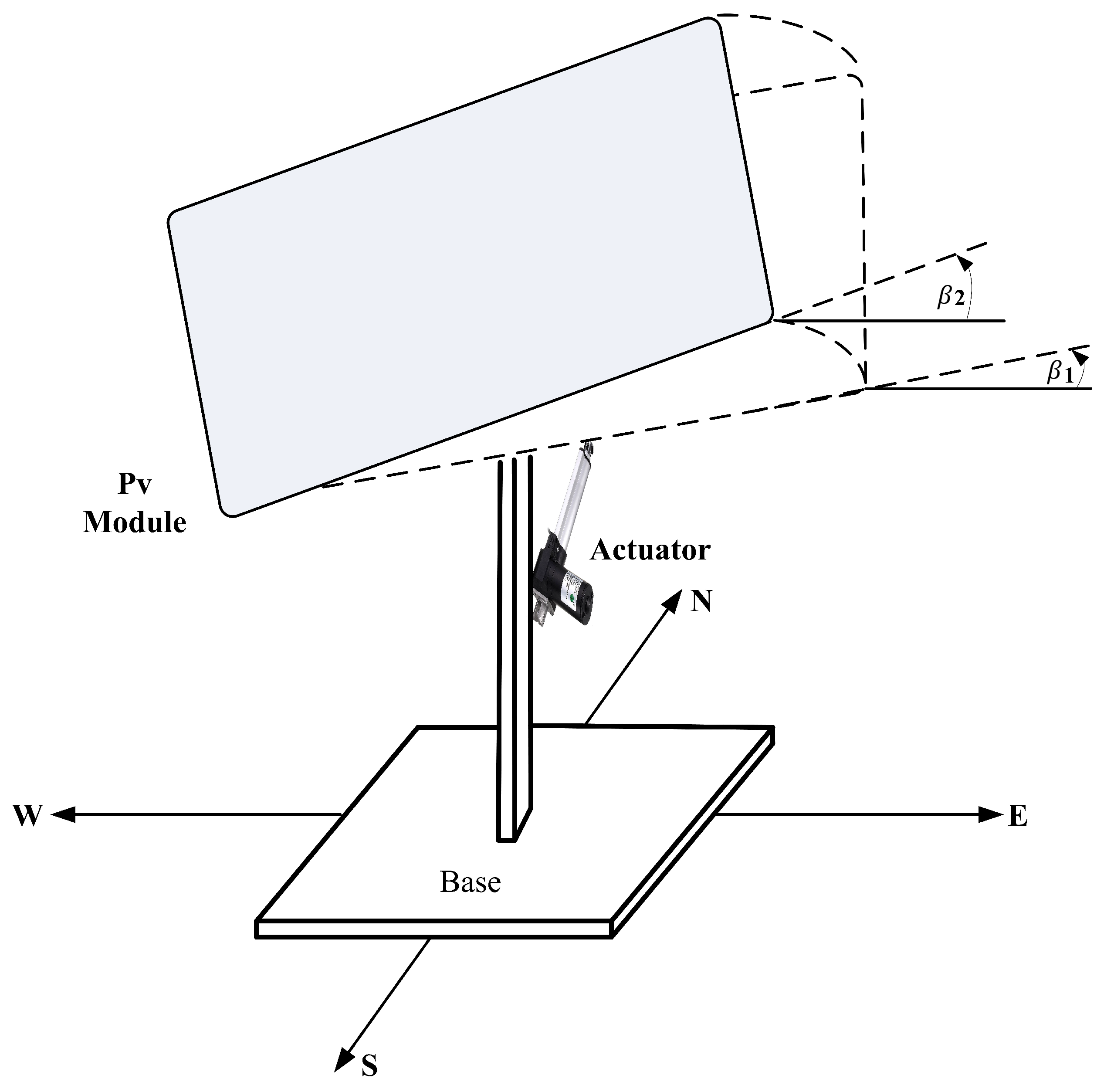
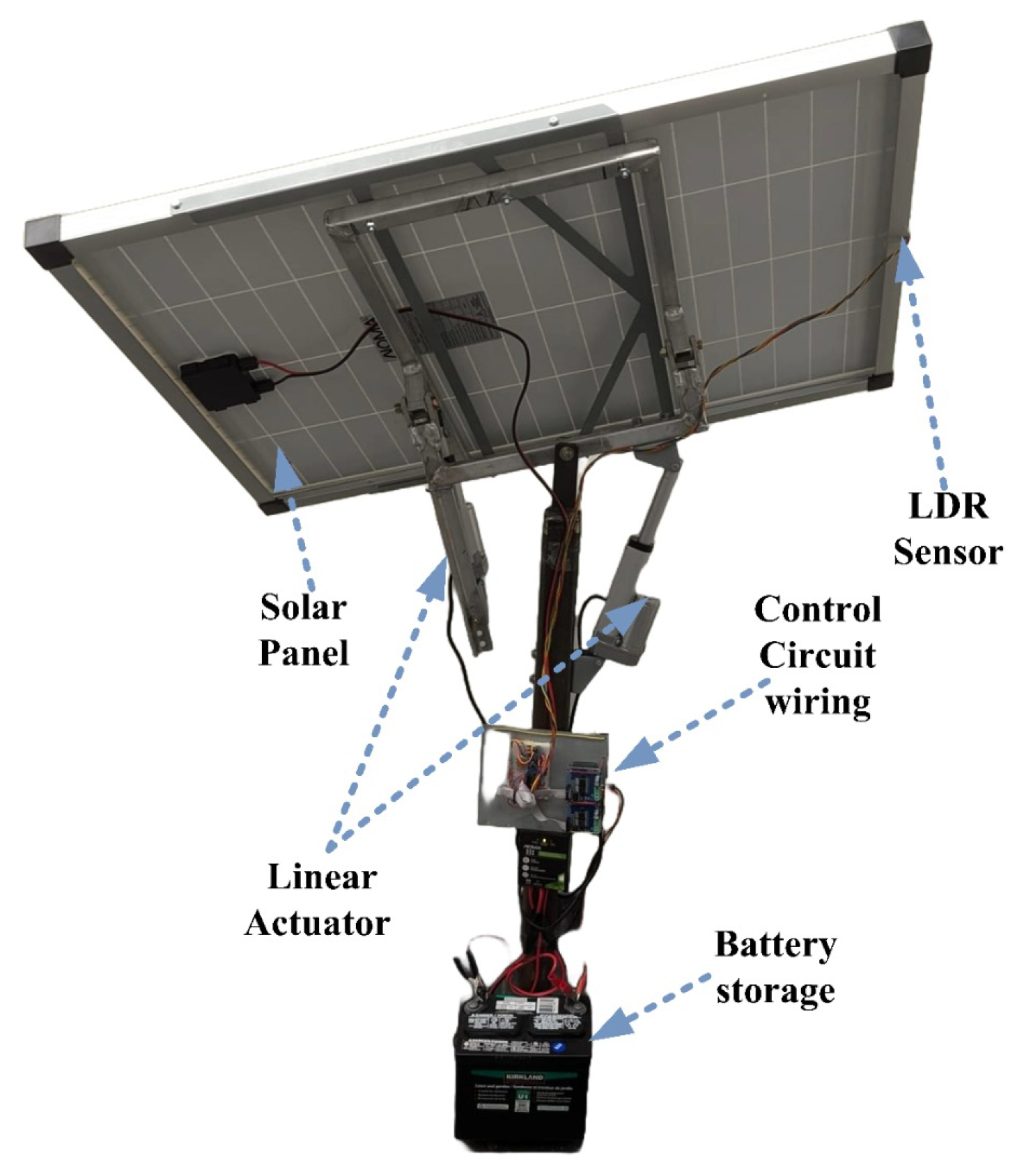
2.1. Physical Structure Design

The structure consists of two main pivot points to move in two dimensions. The first pivot point for motion covers the azimuth angle ($\alpha$) and solar altitude angle ($\beta$) or tilt angle to track the sun even in a continuously changing environment like on the top of a cruise ship and other automotives. Two-axis movement is achieved through the retraction and extension of the linear actuators connected to the system, which converts the 4 inch linear motion into the angular motion of the solar tracking system. These linear actuators are attached on top of each other to control ($\alpha$) and ($\beta$) angles simultaneously. The monopole design provides structural support and covers less base area, which makes it easier to install in small spaces, and it is also cost-efficient. The designed structure is shown in Figure 3.

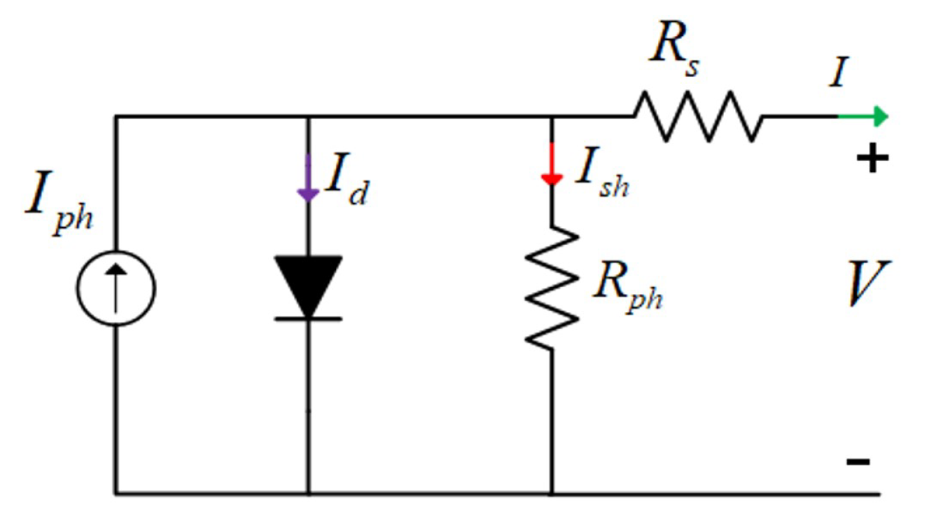
2.2. Modeling of the PV Panel

The photovoltaic diode is used to convert solar energy into electrical energy, so the equivalent circuit of a single solar cell is shown in Figure 4. However, a single cell cannot generate enough energy; that is why the array of multiple solar cells connected in series and parallel act as a single, large PV panel to power up the load [29].

Performing mathematical modeling using Kirchhoff’s current law to determine the output current of a single PV cell is equal to the following:

$$I=I_{ph}-I_r\left(e^{\frac{V+I{R}_s}{nAkT}}-1\right)-{\displaystyle \frac{V}{R_s}},$$

(1)

where V represents the output voltage of PV, $I_r$ is the saturation current, and $I_{p}h$ is the photocurrent. Temperature is T, and k is the Boltzmann constant, where $R_s$ represents the series for shunt resistance.

$$I_{\mathrm{sh}}={\displaystyle \frac{V+I{R}_{\mathrm{s}}}{R_{\mathrm{sh}}}}.$$

(2)

By putting the value from Equation (2) into (1) we get the following:

$$V=nk{T}_{r}ln\left({\displaystyle \frac{I_{ph}+I_r-I_{sh}}{I_r}}\right).$$

(3)

The data sheet of the selected solar panel NOMA(_)011-2514-0 is illustrated in

Table 2. Parameters of the selected PV module.

Specification of PV Under Standard Conditions	Value
Maximum power 100 W Number of cells per module	36
Open-circuit voltage	21.5 V
Short-circuit current	6.1 A
Voltage at maximum power point	17.1 V
Current at maximum power point	5.5 A
Temperature coefficient of Isc	(0.065 ± 0.015) (%)/°C
Temperature coefficient of Voc	−(80 ± 10) mV/°C
Temperature coefficient of power	0.47 ± 0.2 (%)/°C
Operating temperature	−40 °C to 85 °C
Dimensions	100.3 × 67.3 × 3.5 cm
Weight	19 lb/8.7 kg
Power tolerance	±5(%)

.

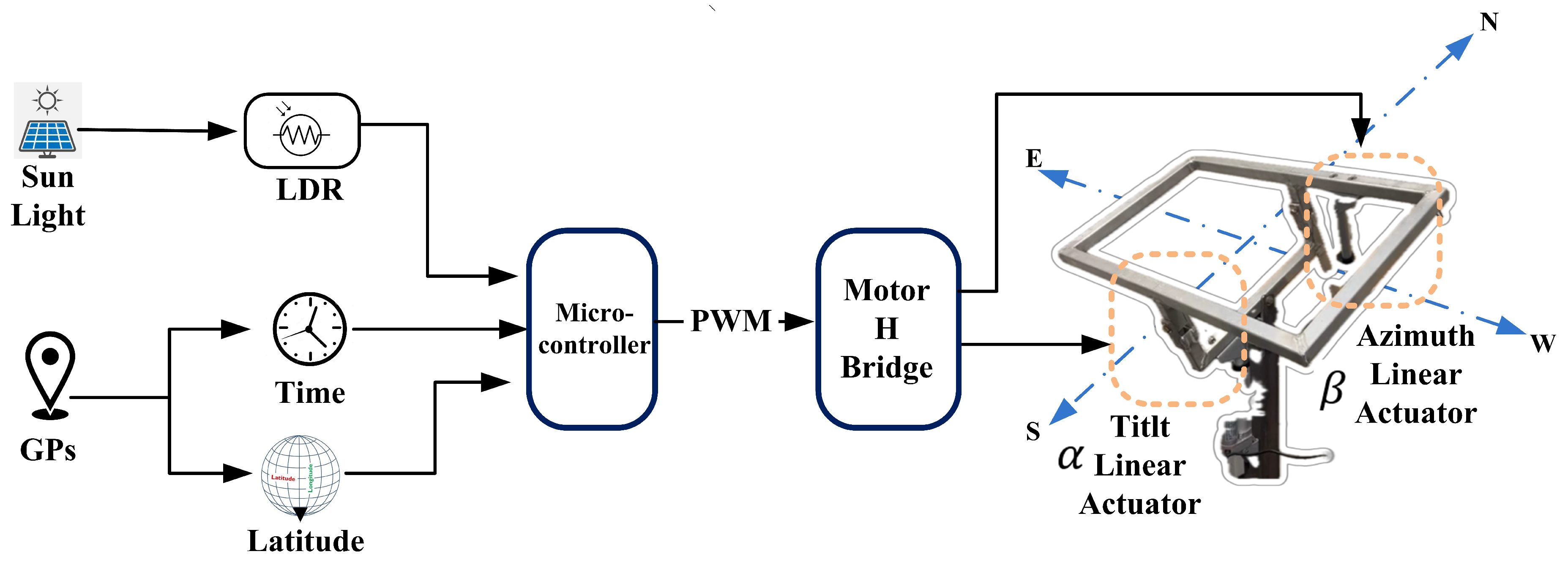
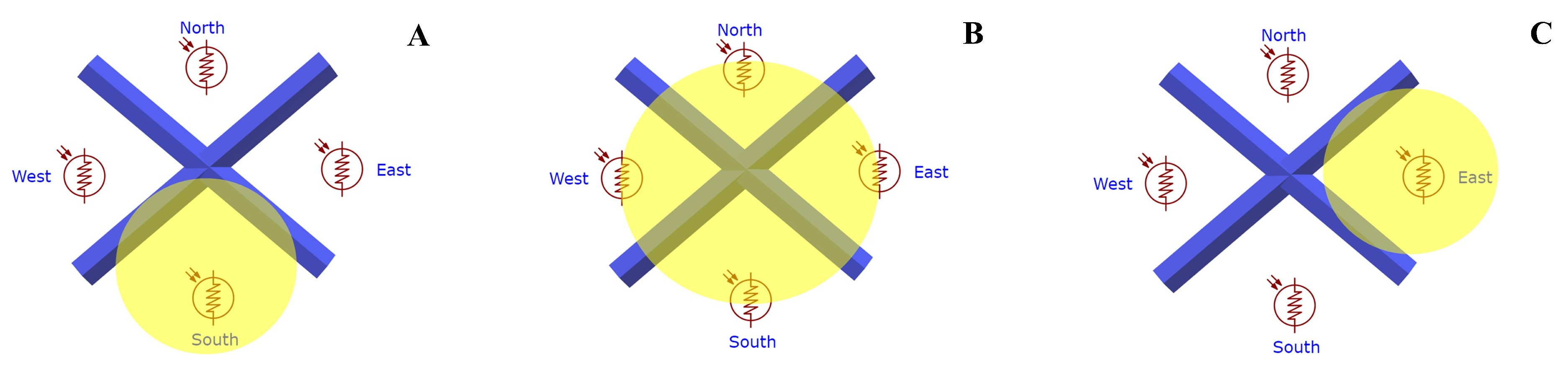
2.3. Solar Tracking System Using a Sensor

The rotation of the Earth on its axis directly affects the apparent motion of sunlight from east to west. In actuality, it is our planet that is orbiting the sun despite the appearance of the opposite. The way that the sun appears to move affects how much power a solar collector receives. The power density on the absorbing surface is equal to the incident power density when the sun’s rays are perpendicular to the surface; although the sun generally swings from east to west, lots of factors affect its precise path throughout the year. One of these factors is the degree of latitude: the sun’s path through the sky is lowered depending on how north or south it is. Also, because of the tilt of the Earth on its axis, the sun’s path changes with the seasons. In the summer, the sun shines higher in the sky than in winter. The solar altitude ($\alpha$), i.e., the angle between the sun’s position and the horizontal plane of the Earth’s surface, and the solar azimuth ($\beta$), the angle between a vertical plane incorporating the solar disk and a line running due north, can be used to determine the location of the sun in the sky with respect to a location on the surface of the Earth, as shown in Figure 5.

2.3.1. Mechanism for Tracking the Sun

The algorithm is designed to operate autonomously. It functions by comparing the average amount of sunlight received by each of the four light-dependent resistors (LDRs). The sun tracking algorithm operates by taking the difference between adjacent LDRs and is programmed using a PID controller to mitigate errors. The LDRs are labeled based on their location: north, south, east, and west [30].

The method determines the average light intensity falling in each direction, providing a positioning sense for the Sun. The mean intensity of the east–west and north–south LDRs are compared first in the procedure. Actuator one turns clockwise if the average intensity of the north LDRs is less than that of the south, and vice versa. When the average light intensity in the east exceeds the average sunlight intensity in the west, actuator two rotates clockwise. In order to track azimuth and title angle, the prototype is constructed with two DC linear actuators, as illustrated in Figure 6. In theory, the actuators may be directly powered by the controller battery storage integrated into the same circuit, but in practice, they are powered separately by the microcontroller.

For sunlight tracking, the naming represents the universal movement of the Sun concerning compass directions; therefore, north and south will be responsible for controlling linear actuator-1 for tilt, one connected to adjusting the azimuth angle, while the east and west sensors are responsible for linear actuator-2 for the azimuth angle. The tracking algorithm uses the difference of two values with the absolute error value to find the sun’s location. All the sensors are separated so that this separation will not allow light to penetrate through, so the resistors will maintain the change in the resistivity to adjust the angle of the panel accordingly. The effect of sunlight on various sensors is illustrated in Figure 7.

Error on the X-axis (horizontal):

errorX = LDRW − LDRE.

Error on the Y-axis (vertical):

errorY = LDRN − LDRS.

The sensor uses the voltage divider principle because static charge can cause an error in the values; therefore, all the pins are grounded by 10 K resistors, also known as pull-down resistors, as shown in Figure 8. The complete light sensor module contains four of these circuits, and these four LDRs use four analog input pins of the microcontroller. The analog input pins of the Arduino (microcontroller) are 10-bit; therefore, the variation will be $2^{10}$, which is from 0 to 1023, and the resistivity represents the light intensity.

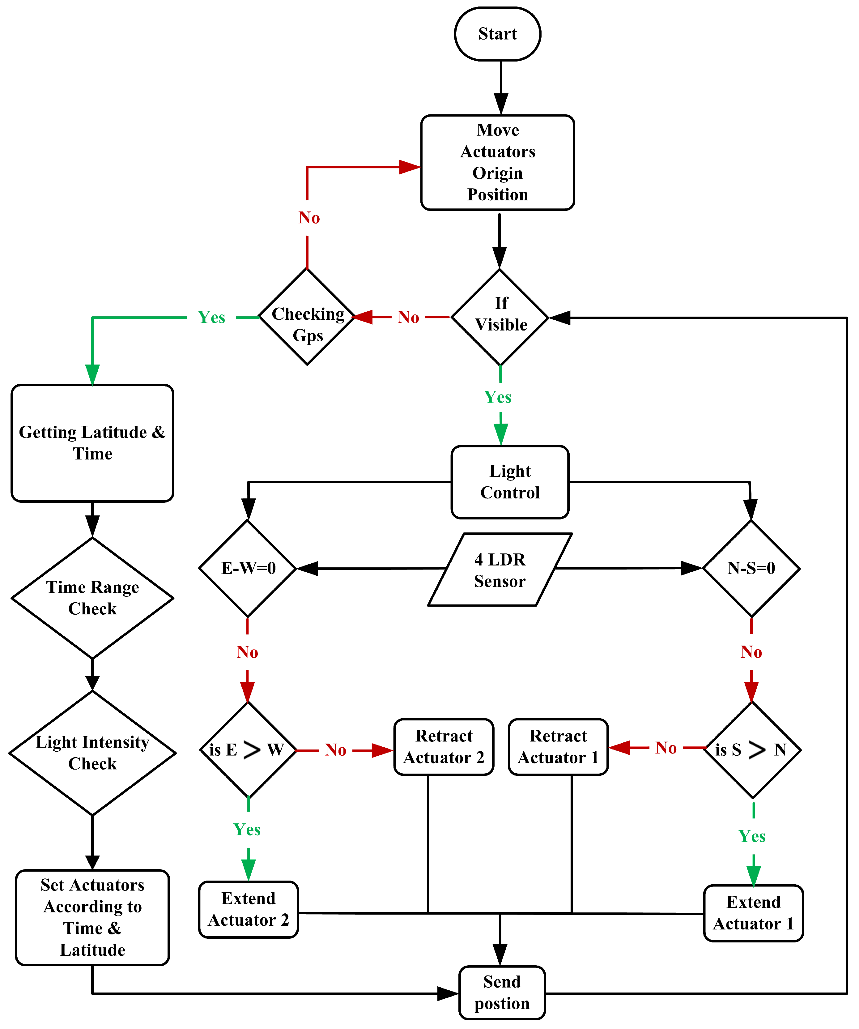
2.3.2. Algorithm Design

The control algorithm works by comparing the two LDR values for both axes: x-axis movement (azimuth) and y-axis movement (tilt). To ensure the solar panel’s position always faces the sun’s position, the mean for both angles should be zero. To maintain this mean, we use a PID controller by moving both actuators. The control algorithm is illustrated in Figure 9 below.

The algorithm uses the comparison of the difference to find the output pin, as shown in

Table 3. Different cases for the control of actuators.

LDR1 (North)	LDR2 (South)	LDR3 (West)	LDR4 (East)	X Axis Action	Y Axis Action
1	1	1	1	Stop	Stop
1	1	1	0	Extend	Retract
1	1	0	1	Retract	Extend
1	1	0	0	Extend	Extend
1	0	1	1	Retract	Retract
1	0	1	0	Extend	Retract
1	0	0	1	Retract	Extend
1	0	0	0	Extend	Extend
0	1	1	1	Retract	Retract
0	1	1	0	Extend	Retract
0	1	0	1	Retract	Extend
0	1	0	0	Extend	Extend
0	0	1	1	Retract	Retract
0	0	1	0	Extend	Retract
0	0	0	1	Retract	Extend
0	0	0	0	Stop	Stop

.

The system working principle tuning cases begins with the first condition to check whether the light is available by comparing it to the minimum thrust–hold value. If that condition is not satisfied, the system will move toward a time-based approach by getting the time and latitude from the GPS module. The first approach is as follows: if light is available, find the difference between two opposite sensors (north LDR and south LDR; east LDR and west LDR). This difference is used to find the error by using the PID controller. The difference between north and south is responsible for the change in altitude ($\alpha$), and between east and west is for the azimuth angle ($\beta$). These angles are controlled by the movement of actuator 2 and actuator 1, respectively.

The second approach uses time-based control; therefore, the initial check will be regarding time, which should be in the range between sunrise and sunset. Then, the light sensitivity check will check whether there is enough light to generate energy or not, and after that, the time-based algorithm will calculate the altitude ($\alpha$) and azimuth ($\beta$) angles to control both actuators concerning the angles calculated by the time-based algorithm. The close loop feedback of the PID is used to maintain the gain out of the output in such a way that we can always make error X and error Y equal to zero. The block diagram of the PID is illustrated in Figure 10.

Error with PID gain on the x-axis: OutputX = Kp x errorX + Ki x integralX + Kd x derivative.

Error with PID gain on the y-axis: OutputY = Kp x errorY + Ki x integralY + Kd x derivativeY.

PID controllers are regarded as the best. PID, or proportional–integral–derivative, is a class of devices used in industrial settings to control temperature, flow, pressure, and speed, among other process factors. A PID controller, as the name implies, combines additional integral and derivative alterations with proportional control to help the device automatically adjust for changes in the system. A control-loop feedback device controls every process variable in this controller. PID controllers maintain the output between the process variable and the setpoint or desired output error-free by using closed-loop techniques.

The three PID controller parameters (proportional, integral, and derivative) must be tuned in order for the controller to function as intended. The literature suggests a number of PID controller tuning and design techniques. Three general categories can be used to group PID design methods:

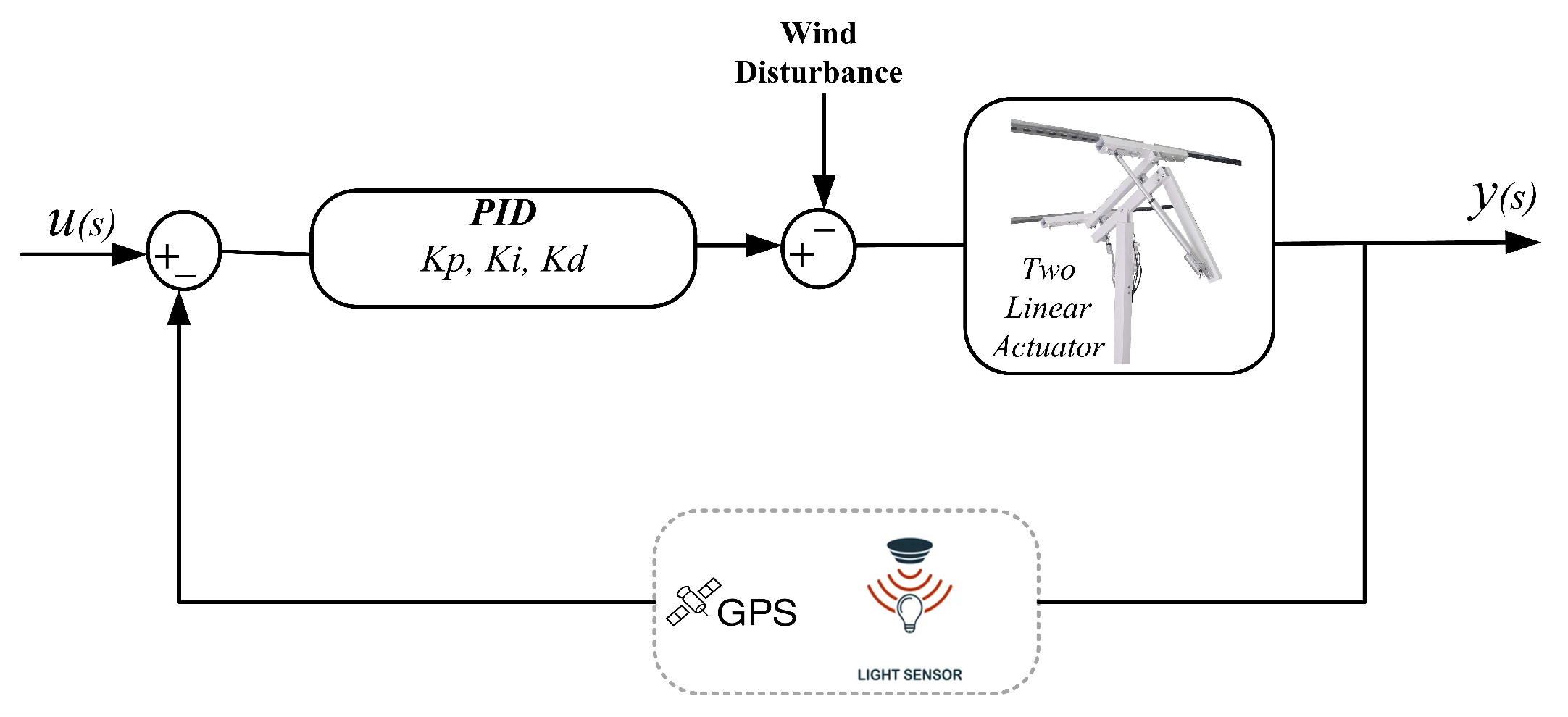
• PID control according to output/input response;
• PID control according to process model;
• PID control according to algorithmic optimization.

State–space or transfer function models are examples of the process models needed for controller design in model-based PID design. Designing for the phase margin and gain is part of the model-based design approach.

Figure 11 depicts the IMC closed-loop control structure, where $G_s$ is the matching transfer function model, $C_{(IMC.S)}$ is the transfer function of the IMC controller, and $G_{sis}$ is the transfer function of the unstable process. The IMC controller $C_{(IMC.S)}$ is equivalent to the IMC principle. Here, a PID controller is used alongside a first- or second-order filter. The PID tuning and testing values are give in the

Table 4. All the tuning cases of the system’s PID controller.

Case	Kp	Ki	Kd	Description
1	1.0	0.02	0.05	Standard values for initial testing.
2	0.5	0.01	0.02	Lower values for smoother control response.
3	2.0	0.05	0.10	Higher values for more aggressive control action for faster response.
4	1.0	0.02	0.01	Higher derivative gain for better stability.
5	1.0	2.0	3.0	Higher integral action for aggressive control.
6	1.0	2.0	3.0	Balanced increase in Kp with standard Ki and Kd.

.

2.4. Time-Based Control of the System

The time-based control of the system is done by using GPS to get real-time latitude and time data and adjust the angle of the solar panel according to the given time, date, and latitude.

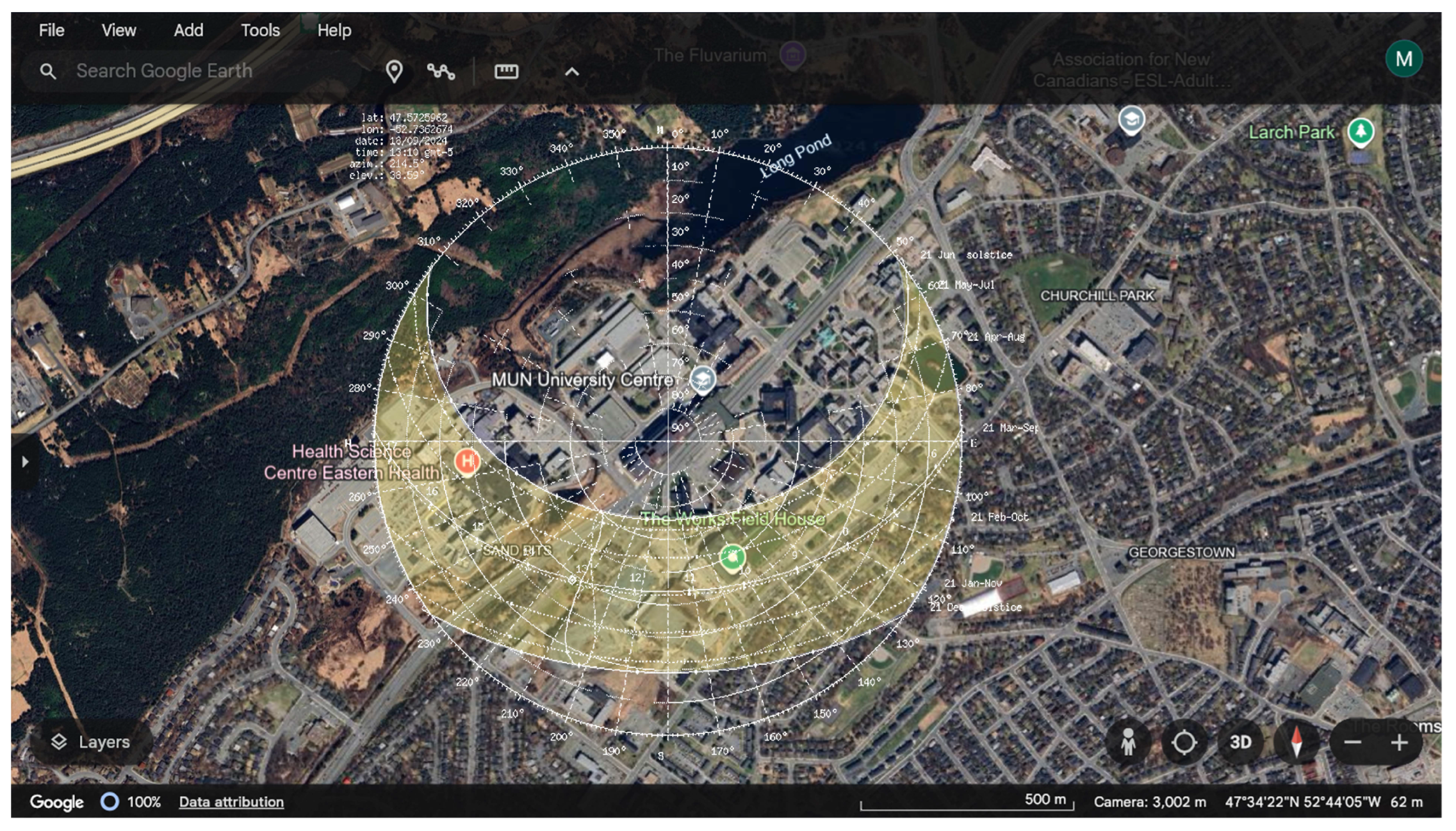
2.4.1. Determining the Decline Angle and Time-Algorithmic Formula

As long as the azimuth and elevation angles are known, every point on the celestial sphere can be located using the horizon coordinate system. The elevation angle is the difference between the ground plane and the sun’s incidence direction. The angle formed by the sun’s rays projected upon the earth and the local median is known as the azimuth angle, which indicates the direction of the Sun [31]. Both the declination angle and the hour angle determine the precision of the elevation angle and azimuth angle. Selecting the proper declination formula and equation of solar time determines the accuracy of the elevation angle and azimuth angle. The accuracy of the hour angle and declination angle is determined by Equations (1) and (2) [32]. Solar declination ($\delta$) is determined as follows:

$$\delta =sin\left({\displaystyle \frac{360}{365.25}}\right)·sin\left(23.44\right)·cos\left({\displaystyle \frac{360}{\pi }}·(d+10)\right)+0.0167·sin\left({\displaystyle \frac{360}{365.25}}·(d-2)\right),$$

(4)

where d is the day of the year (1 to 365 or 366 for leap years). The hour angle measures the Sun’s position relative to the observer’s meridian. It changes throughout the day. The simple formula is as follows:

$$H={15}^{\circ }·(T_{\mathrm{actual}}-12),$$

(5)

$$T_{\mathrm{actual}}=T_{\mathrm{offset}}+t,$$

(6)

where t is equal to the LST and is more accurate. The total offset (in minutes) in the solar time will be the addition of two corrections:

$$T_{\mathrm{offset}}=E_{\mathrm{ot}}+\mathrm{LatiV}\left(\mathrm{minute}\right),$$

(7)

$$\begin{array}{c}\hfill E_{\mathrm{ot}}=229.18\ast \left[0.000075+0.001868cos\left(\gamma \right)-0.032077sin\left(\gamma \right)\right.\\ \hfill \left.-0.014615cos\left(2\gamma \right)-0.040849,sin\left(2\gamma \right)\right]\end{array}$$

(8)

$$\gamma ={\displaystyle \frac{2\ast \pi }{365}}\left[\mathrm{days}-1+{\displaystyle \frac{\mathrm{hour}-12}{24}}\right],$$

(9)

$$\mathrm{LatiV}=4\left[\mathrm{latitude}-15\ast \Delta \mathrm{TZ}\right],$$

(10)

where $\Delta$TZ is the difference in the local time zone to the universal time (UTC). The longitude latitude is measured in degrees and is negative to the west. Here, h is the solar hour angle, and LST is the local solar time in a 24 h format.

The altitude angle ($\beta$) represents the Sun’s elevation above the horizon. It can be calculated using the following equations:

$$sin\left(\beta \right)=sin\left(\varphi \right)·sin\left(\delta \right)+cos\left(\varphi \right)·cos\left(\delta \right)·cos\left(H\right),$$

(11)

$$\beta ={sin}^{-1}\left[sin\left(\varphi \right)·sin\left(\delta \right)+cos\left(\varphi \right)·cos\left(\delta \right)·cos\left(H\right)\right],$$

(12)

where $\beta$ is the solar elevation angle, $\delta$ is the declination angle, $\varphi$ is the latitude of the location, and h is the solar hour angle.

The azimuth angle ($\alpha$) indicates the Sun’s direction (measured clockwise from the north). It can be found using the following equations:

$$cos\left(\alpha \right)=cos\left(\beta \right)·cos\left(\varphi \right)-sin\left(\alpha \right)·sin\left(\varphi \right)-sin\left(\delta \right),$$

(13)

$$\alpha ={cos}^{-1}\left(cos\left(\beta \right)·cos\left(\varphi \right)-sin\left(\alpha \right)·sin\left(\varphi \right)-sin\left(\delta \right)\right).$$

(14)

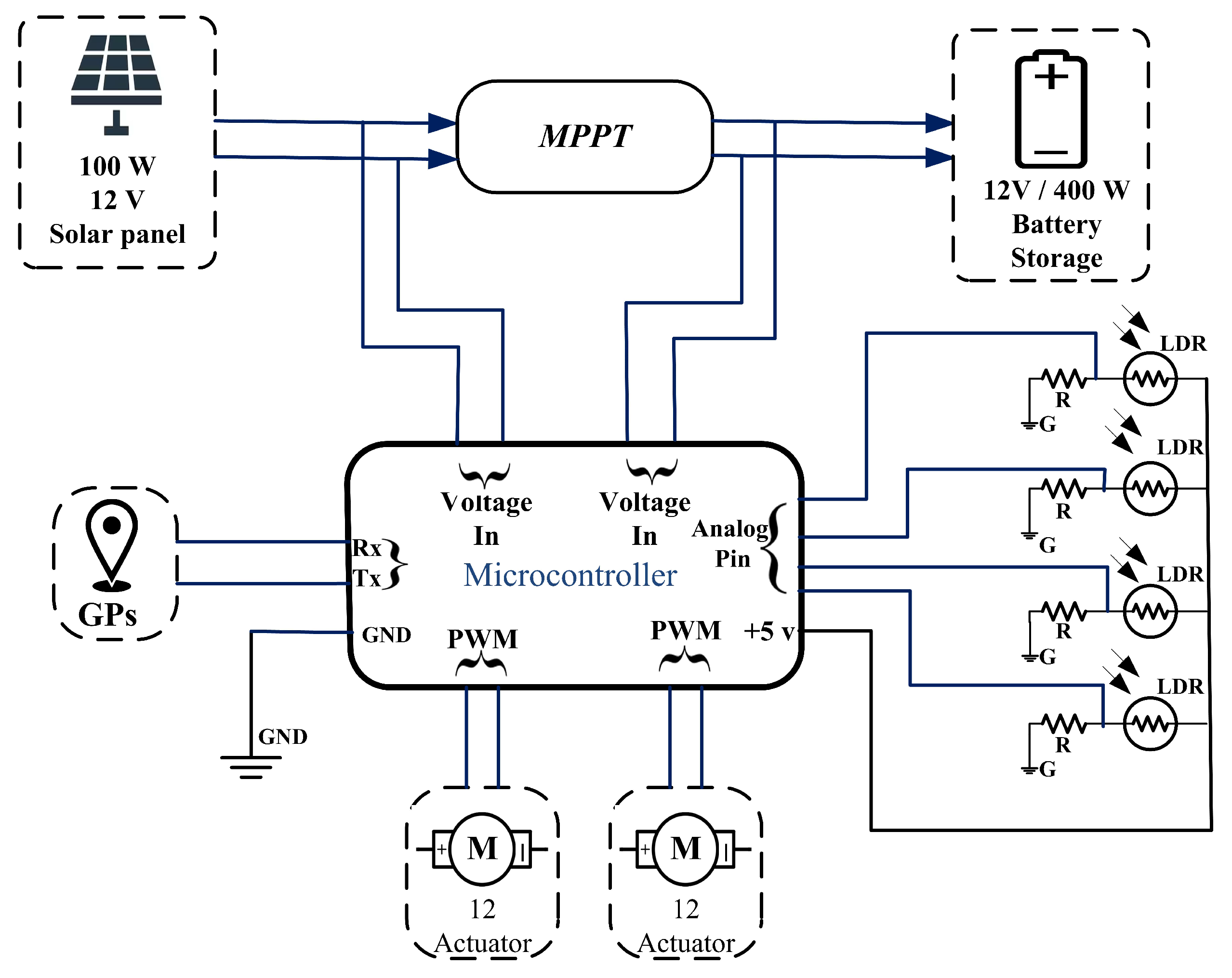
2.4.2. Systems Methodology

The time-based algorithm works by getting the accurate time to measure both axis angles for the solar tracking system. We are using the BE-180 GPS module to get the latitude and time to measure those angles. Then, the acquired time and latitude values will be used in Equations (12) and (14) to find both angles, as illustrated in

Table 5. The change in the angles of both axes with respect to the time in St. John’s, NL, Canada.

Time	Azimuth	Altitude	Position
5:12	86.7	0	Sunrise
6:00	95.41	7.08
7:00	106.95	16.98
8:00	119.65	26.26
9:00	134.32	34.33
10:00	151.62	40.42
11:00	171.39	43.63
11:24	179.84	43.93	Noon
12:00	192.11	43.3
13:00	211.51	39.51
14:00	228.3	32.99
15:00	242.56	24.65
16:00	254.98	15.21
17:00	266.37	5.22
17:35	273	0	Sunset

.

Figure 12 illustrates the movement of the Sun to optimize solar light capture. This figure displays the complete daily cycle of the sun in St. John’s, NL, Canada, highlighting the angles between sunrise and sunset. By tracking these angles, the figure demonstrates how solar panels can be positioned to maximize sunlight exposure by adjusting the azimuth and altitude actuators throughout the day.

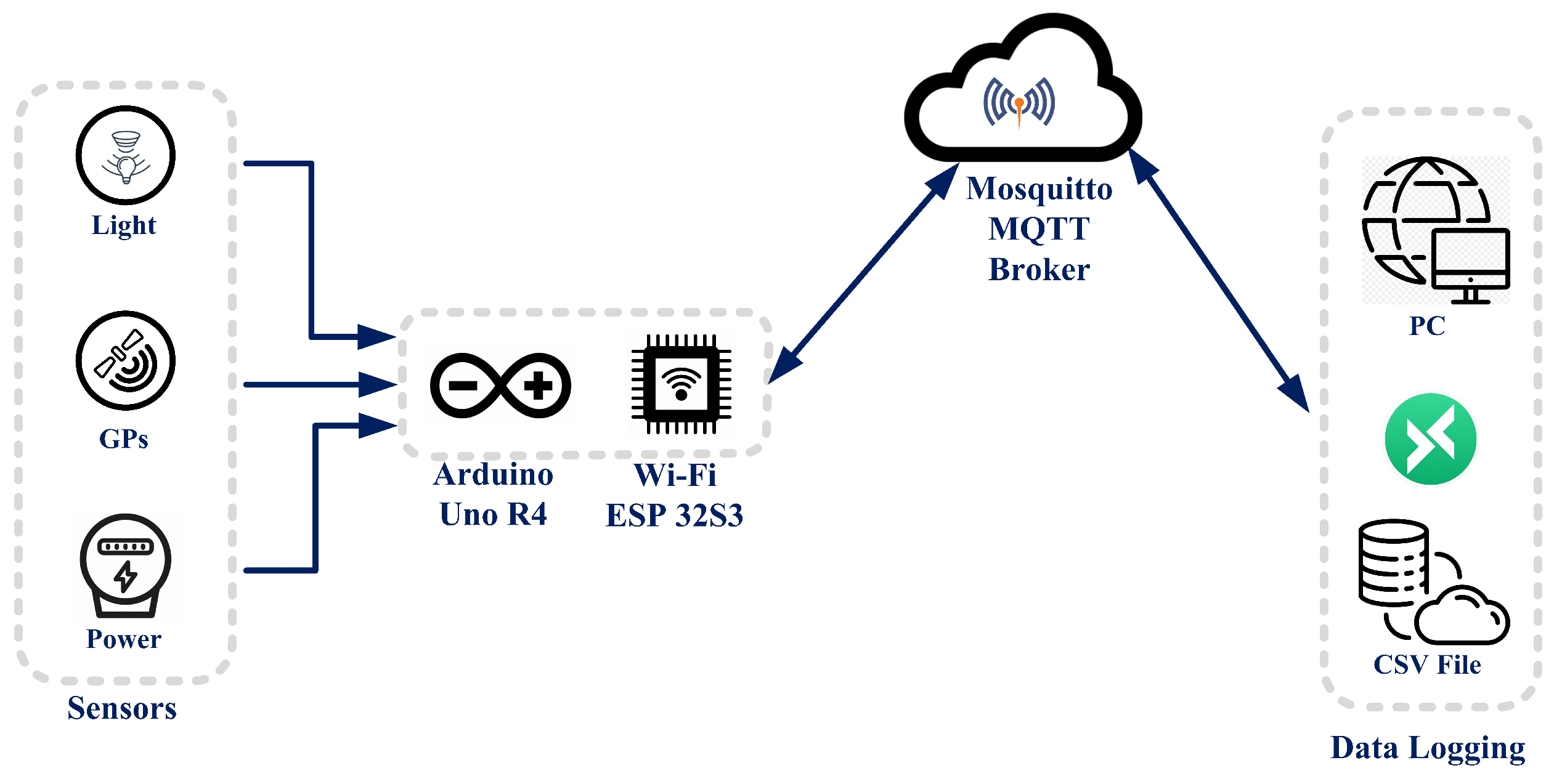
2.4.3. IoT Cloud Server

In order to collect real-time GPS coordinates and determine the power generated accurately through the solar panel for comparison and data collection, we set up an IoT network using an Arduino R4 microcontroller, a Beitian BE-180 GPS module, acs712 current sensor, and a voltage sensor.

The network is based on the message queuing telemetry transport protocol (MQTT). This protocol is very lightweight and was specially designed for machine-to-machine communication. Therefore, most IoT devices use this protocol to send and receive data over a secure SSL network. The messages on this protocol can be only two bytes long, making it easily scalable without the expenditure of more power.

Real-Time GPS and Solar Panel Data Collection Using an IoT Network:

The following steps outline the process of collecting real-time GPS coordinates and determining the power generated by a solar panel using an IoT network. The system is designed for efficient data collection, comparison, and analysis.

1. System Setup: The system uses an Arduino R4 Wifi microcontroller, a Beitian BE-180 GPS module, an ACS712 current sensor, and a voltage sensor to collect real-time data. These components work together to gather the following information:

• GPS coordinates: latitude and longitude values for location tracking.
• Voltage and current: key parameters to determine the power generated by the solar panel.
• Time: for temporal analysis and logging.

2. IoT Network Configuration: An MQTT-based IoT network is used for data transmission. The MQTT protocol is lightweight, making it suitable for low-power, scalable machine-to-machine communication. It operates over a secure SSL connection and allows devices to exchange compact messages efficiently.

3. How MQTT Works: The MQTT network follows a client–server model:

• Clients: devices that can either publish (send) or subscribe to (receive) messages on specific “topics”.
• Broker: a server that facilitates communication between clients.

In this setup,

• the Arduino R4 solar node acts as a publisher, sending data such as time, latitude, voltage, and current to the broker under a specific topic (e.g., the solar tracker).
• the MQTT Mosquitto broker manages the communication, ensuring reliable data transmission between devices.

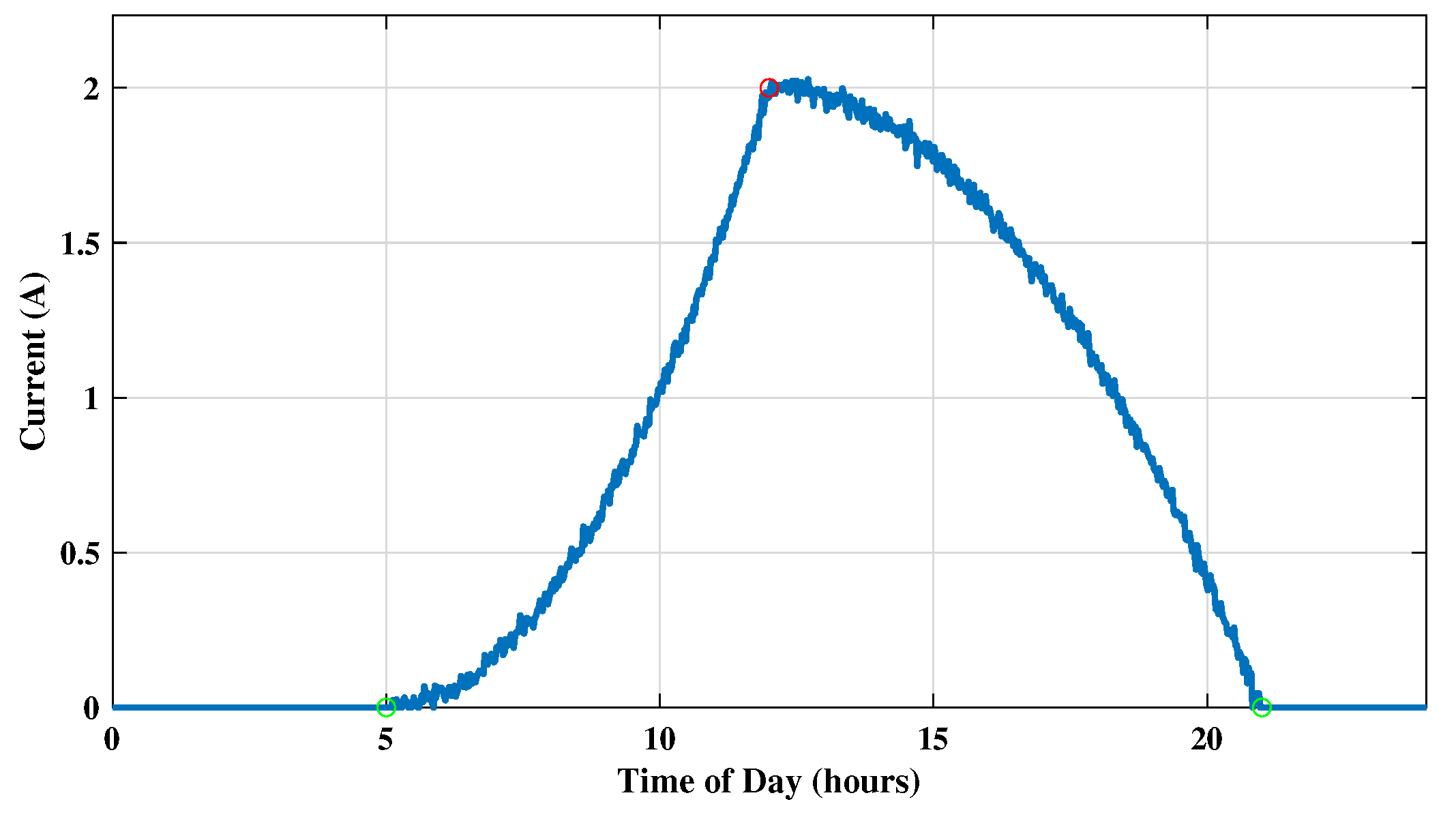
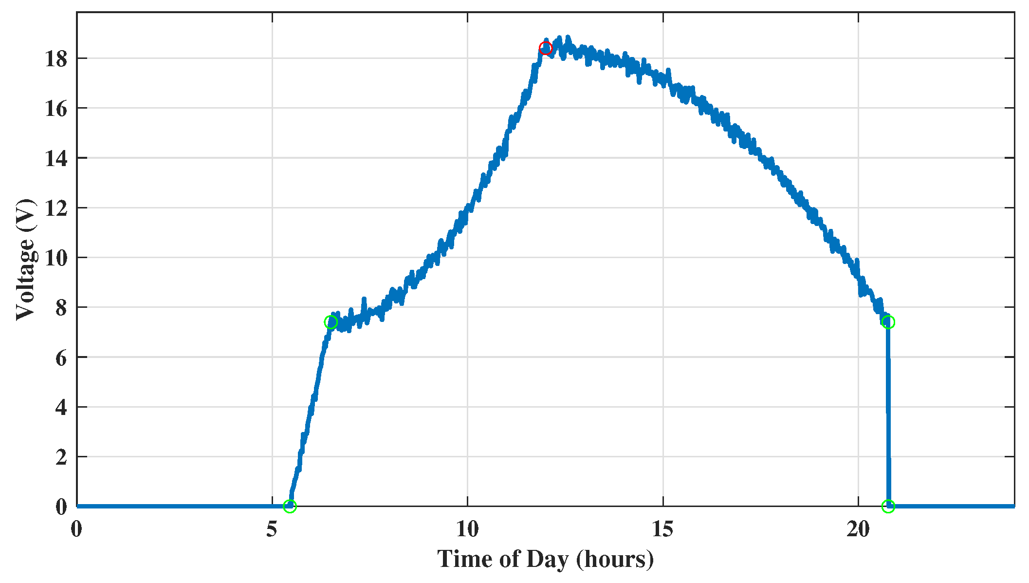
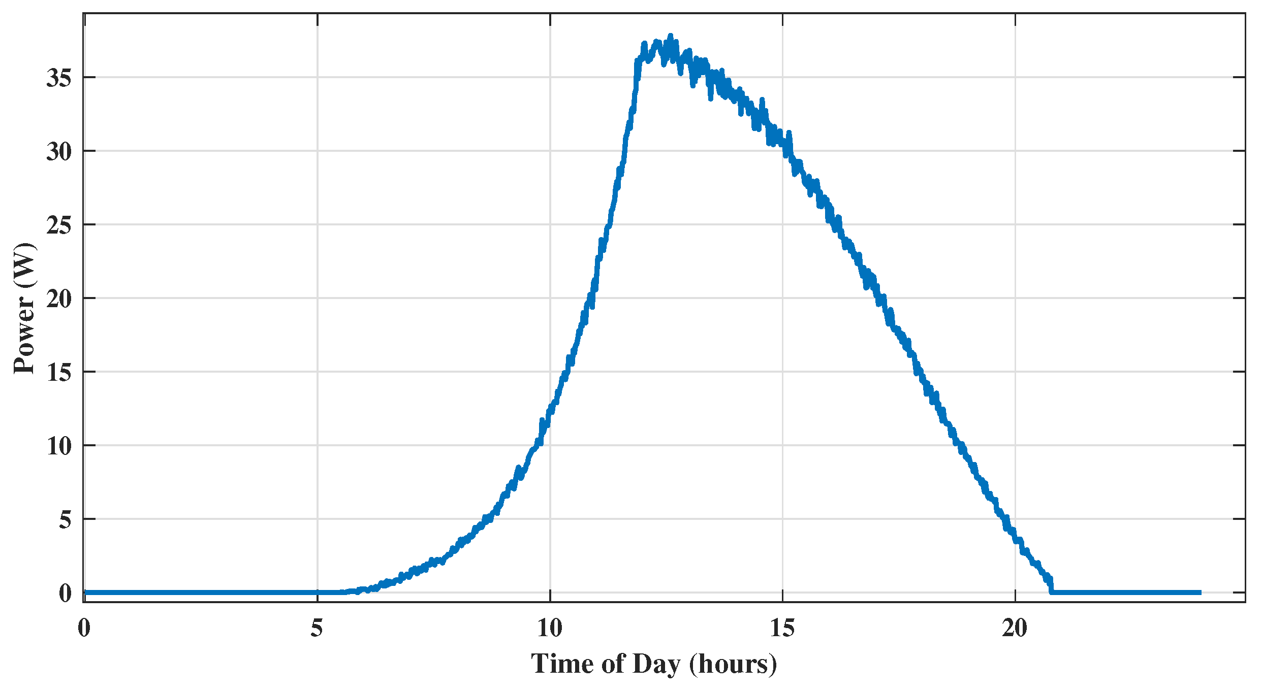
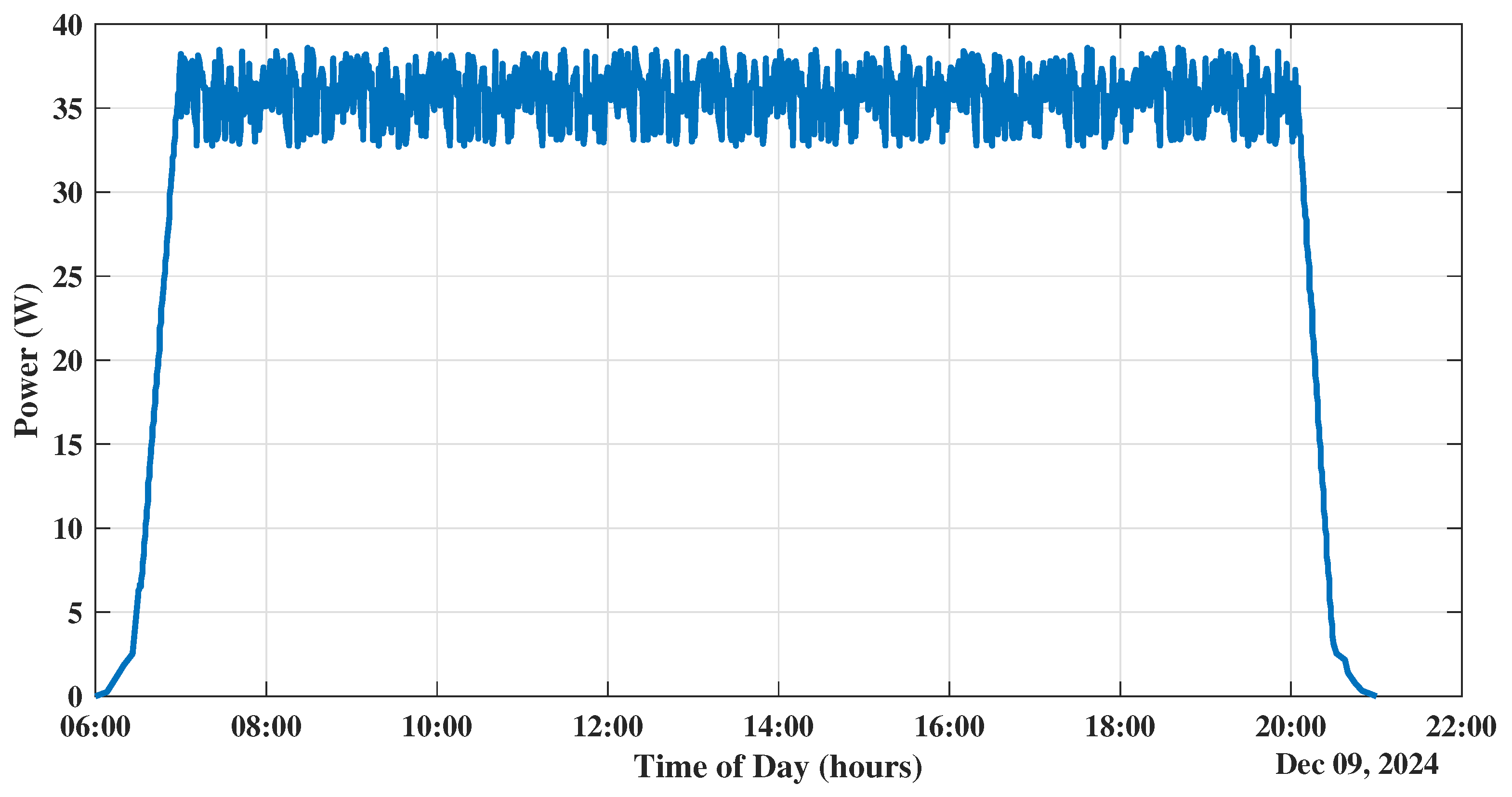
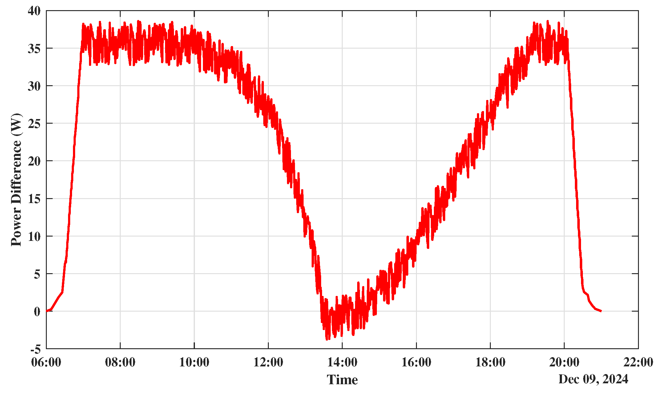
4. Data Logging: A second MQTT client, implemented using the MQTTX Windows app, subscribes to the same topic to receive published data. This client logs the data into a CSV (comma-separated values) file for further analysis and evaluation.

The working principle of the MQTT network is based on a simple client–server network, where all the clients can either subscribe to or publish the message on the same topic. The broker serves as the server and is used for communication between all the clients. These clients can also subscribe to or publish the same topic from the broker to get the data, as illustrated in Figure 13. In our system, the MQTT client Arduino R4 solar node publishes the data (time, latitude, voltage, and ampere) to the broker under the tag (the topic of the solar tracker) to the MQTT mosquito broker. The second MQTT client is used for data logging using the MQTTX Windows app (1.10.1) to subscribe to the same topic to get the data and store it into a CSV (comma-separated values) file for results and evolution.

3. Results

The results represent the change in the values of the LDR when light comes from a different direction, and how it affects the change in the resistance of the LDR, which can change the 10-bit analog input voltage, as shown in Figure 14.

The prototype structure with important components of the system labeled is illustrated in the structure in Figure 15. All results were obtained in a controlled laboratory environment using high-intensity light under minimal load conditions. A comparative analysis of fixed and tracking solar panel systems clearly demonstrates the performance difference in Figure 16 and Figure 17. The tracking system significantly outperformed the fixed system, highlighting its superior efficiency and effectiveness in harnessing solar energy.

The results of the voltage in the oscilloscope for the solar tracking mode are presented below.

When comparing the performance of dual-axis PV tracking systems with fixed-base PV systems, several key metrics are analyzed to understand the differences in efficiency and power output as illustrated in Figure 18 and Figure 19.

Efficiency: Calculate the efficiency of the dual-axis PV tracking system as a percentage:

$$\mathrm{Efficiency}\left({\eta }_i\right)={\displaystyle \frac{P_{\mathrm{tracking},i}}{P_{\mathrm{fixed},i}}}\times 100.$$

(15)

Difference: Calculate the absolute power difference between the two systems:

$$P_{\mathrm{difference},i}=P_{\mathrm{tracking},i}-P_{\mathrm{fixed},i}.$$

(16)

Power percentage: Calculate how much more power the dual-axis PV tracking system produces on average, relative to the fixed-base system:

$$\mathrm{Extra}\mathrm{Power}\mathrm{Percentage}={\displaystyle \frac{{\sum }_{i=1}^n{P}_{\mathrm{tracking},i}-{\sum }_{i=1}^n{P}_{\mathrm{fixed},i}}{{\sum }_{i=1}^n{P}_{\mathrm{tracking},i}}}\times 100,$$

(17)

where

• n is the total number of time points;
• ${\sum }_{i=1}^n{P}_{\mathrm{tracking},i}$ is the total power from the photovoltaic tracking system at all time points;
• ${\sum }_{i=1}^n{P}_{\mathrm{fixed},i}$ is the total power from the fixed photovoltaic system at all time points.

4. Discussion

As illustrated in Figure 14, laboratory findings show a strong relationship between light-dependent resistor (LDR) resistance and the light incident angle. The resistance of the LDR varies noticeably with the angle of rotation of the light source because all sensors are separated in such a way that only the light at the top of the sensor module will fall equally on each sensor, as illustrated in Figure 7, which affects the analog input voltage. This behavior is explained by the photoconductive characteristics of the LDR, which allow it to dynamically change its electrical resistance in response to changes in the direction of sunlight.

It is very clear how sensitive the LDR is to light when the light source is above the sensor. The maximal exposure to light in this setup results in relatively low resistance for all the LDRs (e.g., no change in direction).

The voltage output of dual-axis tracking and stationary solar systems differs significantly, as both graphs illustrate. The fixed system shows noticeable daily swings and fluctuating voltage levels based on the Sun’s position. In contrast, the dual-axis tracking system maintains a reasonably constant voltage profile. This discrepancy is especially evident at noon when the fixed system has a notable voltage peak. The dual-axis tracking capacity is used to maximize energy capture during whole periods by orienting solar panels toward the light and is responsible for obtaining higher efficiency. As a result, the fixed-based system may experience temporary peaks at noon; however, the dual-axis tracking system consistently delivers a more stable and efficient power output throughout the day as illustrated in Figure 20. This advantage is crucial for optimizing energy production and reducing reliance on grid-supplied electricity.

The power difference in the system is visible in Figure 21. There is a huge difference between the morning and evening time; however, the difference is almost non-existent. The calculation of the efficiency to determine the total difference in the efficiency over a one-day period is around 33.23 without any distractions and shade.

5. Conclusions

This research study effectively utilized real-time sensor data to develop and establish a highly accurate solar tracking system. Through the integration of LDR (light-dependent resistor) sensors and GPS, the system was able to precisely identify the location and orientation of the Sun, thereby enabling the solar panel to maintain optimal alignment throughout the day. This capability ensures that the system can effectively track the Sun’s position and adjust the panel accordingly, contributing to a substantial 33.23% increase in energy production compared to a fixed panel. The system’s tracking accuracy was thoroughly examined, demonstrating its ability to achieve the desired level of precision, such as tracking the Sun within the designated azimuth angle range of 1200 and tilt angle range of 900. According to the findings, the installation of a solar tracking device has significantly increased power generation.

• The dual-axis tracker enhances PV panel energy production by 33.23%.
• IoT integration supports real-time monitoring and system optimization.
• Cost analysis confirms economic viability with a 3.5 to 5-year payback period.
• The environmental impact is minimized through efficient land use.

References

1. Wang, J.M.; Lu, C.L. Design and implementation of a sun tracker with a dual-axis single motor for an optical sensor-based photovoltaic system. Sensors 2013, 13, 3157–3168. [Google Scholar] [CrossRef] [PubMed]
2. Abdullah, M.Z.; Sudiharto, I.; Eviningsih, R.P. Photovoltaic system MPPT using fuzzy logic controller. In Proceedings of the 2020 International Seminar on Application for Technology of Information and Communication (iSemantic), Semarang, Indonesia, 19–20 September 2020; IEEE: Piscataway, NJ, USA, 2020; pp. 378–383. [Google Scholar]
3. van Sark, W.G.; Muizebelt, P.; Cace, J.; de Vries, A.; de Rijk, P. Grid parity reached for consumers in the Netherlands. In Proceedings of the 2012 38th IEEE Photovoltaic Specialists Conference, Austin, TX, USA, 3–8 June 2012; IEEE: Piscataway, NJ, USA, 2012; pp. 002462–002466. [Google Scholar]
4. Candelise, C.; Winskel, M.; Gross, R.J. The dynamics of solar PV costs and prices as a challenge for technology forecasting. Renew. Sustain. Energy Rev. 2013, 26, 96–107. [Google Scholar] [CrossRef]
5. Allington, L.; Cannone, C.; Pappis, I.; Barron, K.C.; Usher, W.; Pye, S.; Brown, E.; Howells, M.; Walker, M.Z.; Ahsan, A.; et al. Selected ‘Starter kit’energy system modelling data for selected countries in Africa, East Asia, and South America (# CCG, 2021). Data Brief 2022, 42, 108021. [Google Scholar] [PubMed]
6. Borhanazad, H.; Mekhilef, S.; Saidur, R.; Boroumandjazi, G. Potential application of renewable energy for rural electrification in Malaysia. Renew. Energy 2013, 59, 210–219. [Google Scholar] [CrossRef]
7. Juswanto, W. Renewable Energy and Sustainable Development in Pacific Island Countries; ADB Institue: Tokyo, Japan, 2016. [Google Scholar]
8. Birol, F. Energy Is at the Heart of the Sustainable Development Agenda to 2030; IEA: Paris, France, 2021. [Google Scholar]
9. Azam, M.S.; Bhattacharjee, A.; Hassan, M.; Rahaman, M.; Aziz, S.; Shaikh, M.A.A.; Islam, M.S. Performance enhancement of solar PV system introducing semi-continuous tracking algorithm based solar tracker. Energy 2024, 289, 129989. [Google Scholar] [CrossRef]
10. Rajesh, T.; Tamilselvan, K.; Vijayalakshmi, A.; Kumar, C.N.; Reddy, K.A. Design and implementation of an automatic solar tracking system for a monocrystalline silicon material panel using MPPT algorithm. Mater. Today Proc. 2021, 45, 1783–1789. [Google Scholar] [CrossRef]
11. Chander, M.; Chopra, K.; Joshi, J.; Mukerjee, A. Comparative study of different orientations of photovoltaic system. Sol. Wind Technol. 1988, 5, 329–334. [Google Scholar] [CrossRef]
12. Ramamurthy, V.; Tiku, P.; Radhamohan, V.; Rao, M. Evaluation of outdoor performance of polycrystalline silicon photovoltaic panel. In Proceedings of the 6th International Photovoltaic Science and Engineering Conference, New Delhi, India, 10–14 February 1992; pp. 10–14. [Google Scholar]
13. Jamroen, C.; Komkum, P.; Kohsri, S.; Himananto, W.; Panupintu, S.; Unkat, S. A low-cost dual-axis solar tracking system based on digital logic design: Design and implementation. Sustain. Energy Technol. Assess. 2020, 37, 100618. [Google Scholar] [CrossRef]
14. Zhu, Y.; Liu, J.; Yang, X. Design and performance analysis of a solar tracking system with a novel single-axis tracking structure to maximize energy collection. Appl. Energy 2020, 264, 114647. [Google Scholar] [CrossRef]
15. Muthukumar, P.; Manikandan, S.; Muniraj, R.; Jarin, T.; Sebi, A. Energy efficient dual axis solar tracking system using IOT. Meas. Sens. 2023, 28, 100825. [Google Scholar] [CrossRef]
16. Singh, R.; Kumar, S.; Gehlot, A.; Pachauri, R. An imperative role of sun trackers in photovoltaic technology: A review. Renew. Sustain. Energy Rev. 2018, 82, 3263–3278. [Google Scholar] [CrossRef]
17. Fuentes-Morales, R.F.; Diaz-Ponce, A.; Peña-Cruz, M.I.; Rodrigo, P.M.; Valentín-Coronado, L.M.; Martell-Chavez, F.; Pineda-Arellano, C.A. Control algorithms applied to active solar tracking systems: A review. Sol. Energy 2020, 212, 203–219. [Google Scholar] [CrossRef]
18. Abdollahpour, M.; Golzarian, M.R.; Rohani, A.; Zarchi, H.A. Development of a machine vision dual-axis solar tracking system. Sol. Energy 2018, 169, 136–143. [Google Scholar] [CrossRef]
19. Alhajri, K.; Al Jahdhami, M.A.; El-Saleh, A.A. An overview on solar tracking systems. In Proceedings of the Asia Conference on Electrical, Power and Computer Engineering, Shanghai, China, 22–24 April 2022; pp. 1–6. [Google Scholar]
20. Bukit, F.R.; Sani, A.; Hasugian, I.A.; Butar-Butar, T.D.P. The Affect of Solar Panel Tilt Angle with Reflector on The Output Power Using Calculation and Experimental Methods. In Proceedings of the 2022 6th International Conference on Electrical, Telecommunication and Computer Engineering (ELTICOM), Medan, Indonesia, 22–23 November 2022; IEEE: Piscataway, NJ, USA, 2022; pp. 80–84. [Google Scholar]
21. Stebi, M.A.; Jeyam, A. Estimation of household appliances and monitorization for impact reduction using electro chemical sensor. Int. J. Syst. Des. Comput. 2023, 1, 26–34. [Google Scholar]
22. Fernández-Ahumada, L.; Ramírez-Faz, J.; López-Luque, R.; Varo-Martínez, M.; Moreno-García, I.; De La Torre, F.C. Influence of the design variables of photovoltaic plants with two-axis solar tracking on the optimization of the tracking and backtracking trajectory. Sol. Energy 2020, 208, 89–100. [Google Scholar] [CrossRef]
23. Kavlak, G.; McNerney, J.; Trancik, J.E. Evaluating the causes of cost reduction in photovoltaic modules. Energy Policy 2018, 123, 700–710. [Google Scholar] [CrossRef]
24. Nonhebel, S. Renewable energy and food supply: Will there be enough land? Renew. Sustain. Energy Rev. 2005, 9, 191–201. [Google Scholar] [CrossRef]
25. Rejeb, O.; Radwan, A.; Abo-Zahhad, E.M.; Ghenai, C.; Serageldin, A.A.; Ahmed, M.; El-Shazly, A.A.; Bettayeb, M.; Abdelrehim, O. Numerical analysis of passive cooled ultra-high concentrator photovoltaic cell using optimal heat spreader design. Case Stud. Therm. Eng. 2020, 22, 100757. [Google Scholar] [CrossRef]
26. Badr, F.; Radwan, A.; Ahmed, M.; Hamed, A.M. An experimental study of the concentrator photovoltaic/thermoelectric generator performance using different passive cooling methods. Renew. Energy 2022, 185, 1078–1094. [Google Scholar] [CrossRef]
27. Ma, T.; Li, Z.; Zhao, J. Photovoltaic panel integrated with phase change materials (PV-PCM): Technology overview and materials selection. Renew. Sustain. Energy Rev. 2019, 116, 109406. [Google Scholar] [CrossRef]
28. Taheri, A.; Malayjerdi, M.; Kazemi, M.; Kalani, H.; Nemati-Farouji, R.; Passandideh-Fard, M.; Sardarabadi, M. Improving the performance of a nanofluid-based photovoltaic thermal module utilizing dual-axis solar tracker system: Experimental examination and thermodynamic analysis. Appl. Therm. Eng. 2021, 196, 117178. [Google Scholar] [CrossRef]
29. Tiwari, H.; Ghosh, A. Power flow control in solar PV fed DC Microgrid with storage. In Proceedings of the 2020 IEEE 9th Power India International Conference (PIICON), Sonepat, India, 28 February–1 March 2020; IEEE: Piscataway, NJ, USA, 2020; pp. 1–6. [Google Scholar]
30. Patel, K.; Borole, S.; Ramaneti, K.; Hejib, A.; Singh, R.R. Design and implementation of sun tracking solar panel and smart wiping mechanism using tinkercad. IOP Conf. Ser. Mater. Sci. Eng. 2020, 906, 012030. [Google Scholar] [CrossRef]
31. Huang, M.; Zhou, Z. Solar Tracking and Group Control System Based on EtherCAT. In Proceedings of the 2018 Chinese Automation Congress (CAC), Xi’an, China, 30 November–2 December 2018; IEEE: Piscataway, NJ, USA, 2018; pp. 1959–1962. [Google Scholar]
32. Sproul, A.B. Derivation of the solar geometric relationships using vector analysis. Renew. Energy 2007, 32, 1187–1205. [Google Scholar] [CrossRef]
Figure 1. Block diagram illustrating the proposed hybrid dual-axis solar tracking system, combining real-time sunlight sensing with time-based GPS tracking for optimized solar energy capture.
Energies 18 00217 g001
Figure 2. Electrical circuit diagram of the dual-axis solar tracking system showing connections between sensors, controllers, and actuators.
Energies 18 00217 g002
Figure 3. Mechanical structure of the dual-axis solar tracking system, highlighting the two pivot points for azimuth and altitude adjustments, supported by linear actuators.
Energies 18 00217 g003
Figure 4. Equivalent circuit model of a single photovoltaic (PV) cell used for energy generation, depicting the relationship between the current, voltage, and resistance.
Energies 18 00217 g004
Figure 5. Annual sun path diagram showing the azimuth and tilt angles used for designing the dual-axis tracking system to optimize solar exposure.
Energies 18 00217 g005
Figure 6. Illustration of the solar panel’s angular adjustments enabled by linear actuators for azimuth and tilt tracking based on light intensity changes.
Energies 18 00217 g006
Figure 7. Effect of sunlight on light-dependent resistors (LDRs) under varying conditions: (A) sunlight concentration on the south LDR, (B) balanced sunlight concentration across all LDRs, and (C) sunlight concentration on the east LDR.
Energies 18 00217 g007
Figure 8. Schematic diagram of the light sensor module, showing the connection of LDRs to the microcontroller using pull-down resistors for accurate light-intensity measurement.
Energies 18 00217 g008
Figure 9. Flow diagram of the solar tracking algorithm, illustrating the decision-making processes for adjusting the azimuth and tilt angles based on light intensity and time-based control.
Energies 18 00217 g009
Figure 10. Block diagram of the PID control system for regulating linear actuator movements to ensure precise solar panel tracking.
Energies 18 00217 g010
Figure 11. Internal model control (IMC)-based PID control block diagram for optimizing solar tracking performance, showing control-loop feedback mechanisms.
Energies 18 00217 g011
Figure 12. Daily solar path for St. John’s, NL, illustrating changes in azimuth and altitude angles from sunrise to sunset for optimizing panel positioning.
Energies 18 00217 g012
Figure 13. Flow diagram of the IoT-based data acquisition system for real-time monitoring of GPS coordinates and solar power output.
Energies 18 00217 g013
Figure 14. The change in the analog reading values of all LDR sensors.
Energies 18 00217 g014
Figure 15. Assembled prototype with component labeling.
Energies 18 00217 g015
Figure 16. Current of the PV panel at a fixed position of 30 latitude.
Energies 18 00217 g016
Figure 17. Voltage of the PV panel at a fixed position of 30 latitude.
Energies 18 00217 g017
Figure 18. Power of the PV panel at a fixed position of 30 latitude.
Energies 18 00217 g018
Figure 19. Voltage and current of the PV panel using the solar tracking system.
Energies 18 00217 g019
Figure 20. Power of the PV panel using a solar tracking system.
Energies 18 00217 g020
Figure 21. The difference in the power of both systems.
Energies 18 00217 g021