A Digital Twin of Hot Pumping Waxy Oil Through a Main Pipeline

Abstract

This article presents a digital twin of hot pumping waxy oil through a main pipeline. Digital copies of the original object data were identified through sensor measurements from SCADA and ECMAS, forming the basis of the SmartTranPro 1.7.1 Software. The mathematical model of the software describes the process of hot pumping waxy oil regarding heat exchange with the environment. The intelligent algorithms of the SmartTranPro 1.7.1 Software were used to determine the actual dependencies of the digital twins of the objects, hydraulic parameters, and heat transfer for the Kassymov–Bolshoi Chagan hot main pipeline, which has a length of 450 km. The results of the thermal–hydraulic calculations for the hot pumping of waxy oil are in good agreement with the actual sensor data from SCADA and ECASM. The optimization calculations of the heating temperature for waxy oil show an economic efficiency of 38.9% for the hot pumping method.

1. Introduction

A digital twin is a sophisticated algorithm that predicts the behavior of a natural physical process based on accurate data [1,2,3,4] in order to recommend necessary solutions [5,6]. It can simulate various production processes and predict their operation in natural conditions [7,8,9,10]. By integrating technologies such as the Internet of Things (IoT), data analytics, and artificial intelligence (AI), a digital twin enhances operational efficiency and decision-making processes.

The software receives sensor data from a physical system to create a digital duplicate, facilitating a deeper understanding and analysis of natural objects or systems [11,12]. Users can use digital twins to explore options for improving production processes [13,14,15,16,17] or increasing labor productivity [18,19,20], since they provide data for training, analyzing, and understanding objects and system functions [21,22,23,24,25].

The purpose of digital twins is to detect unacceptable deviations from ideal conditions across multiple parameters. Such a deviation is a reason to optimize the process, improve quality, or increase efficiency. A digital twin displays the production processes, providing a dynamic digital model of a physical object’s historical and current behavior [26,27].

As highlighted in the literature [1,2,3,4,5,6,7,8,9,10,11,12,13,14,15,16,17,18,19,20,21,22,23,24,25,26,27,28,29,30], various issues related to the development of digital twins for industrial production have been analyzed. Notably, only one study [31] provides a detailed description of the pipeline system, including the diagrams, sensors, and measurement instruments placed along the length of the pipelines. The integration of intelligent networks has significantly enhanced oil transportation across broader corporate frameworks, leveraging the sensor network’s cumulative focus on optimizing energy resource utilization [31].

This paper examines a digital twin of the technological process of hot pumping waxy oil through a main pipeline. SCADA (Supervisory Control and Data Acquisition) and ECMAS (Electricity Controlling and Monitoring Automated System) sensors verify the correctness of the source data. The accuracy of the digital twin is assessed by comparing the digital model and the physical objects of the main pipeline.

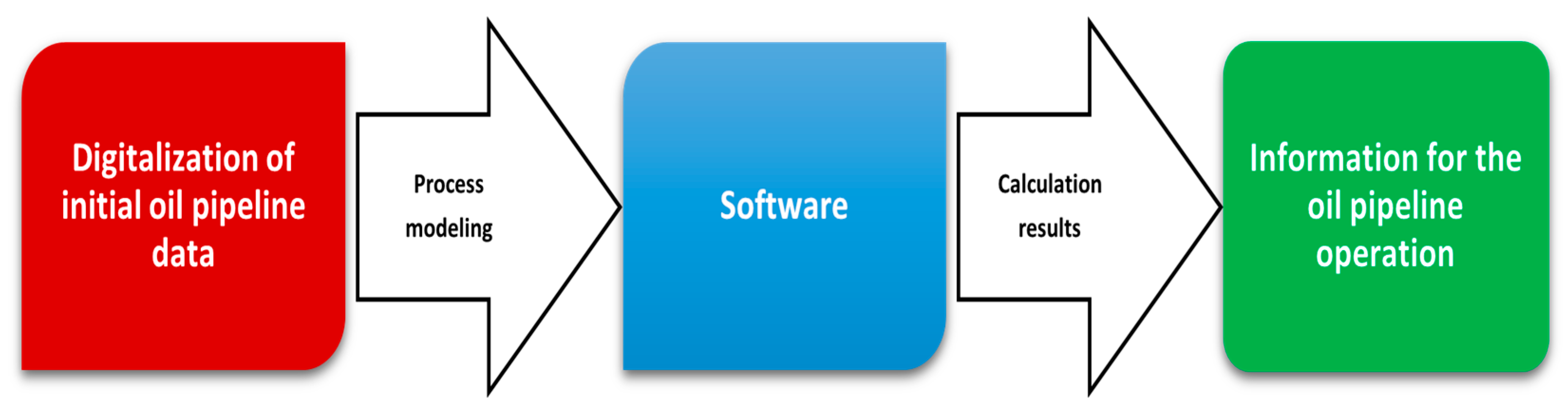
2. Digital Twin of Waxy Oil Hot Pumping

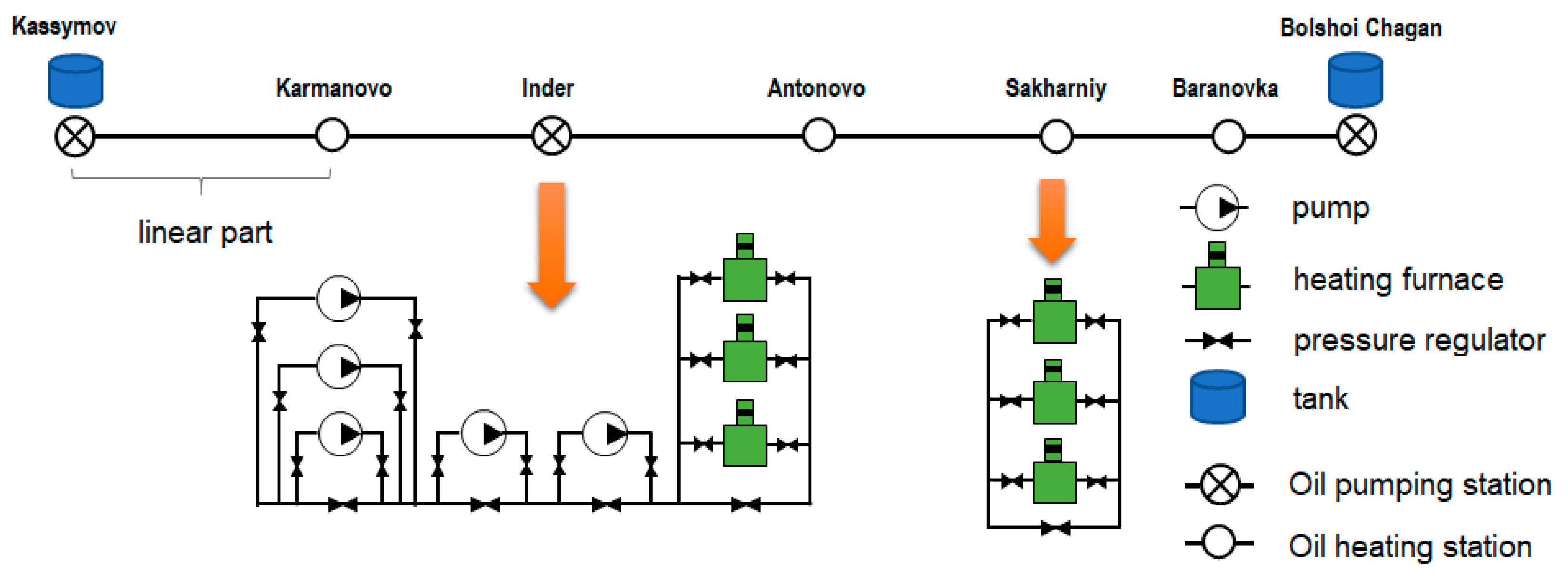
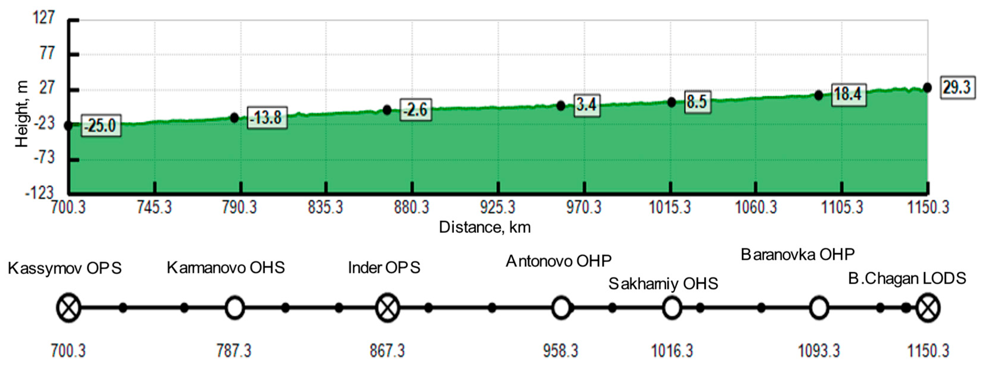
2.1. Structure

Figure 1 demonstrates the digital twin structure, which consists of a database of digitized source data, process modeling, software, calculation results, and oil pipeline operation information.

Figure 2 shows the Kassymov–Bolshoi Chagan main pipeline located in Kazakhstan. It has six linear sections: Kassymov–Karmanovo; Karmanovo–Inder; Inder–Antonovo; Antonovo–Sakharniy; Sakharniy–Baranovka; and Baranovka–Bolshoi Chagan. Each linear section consists of underground pipelines at a depth of H = 1.5 m and shut-off valves. Pumps and heating furnaces are located at the Kassymov, Inder, and Bolshoi Chagan oil-pumping stations (OPS), which have boosters, main pumps, and pressure regulators. Additionally, heating furnaces are located at the Karmanovo, Antonovo, Sakharniy, and Baranovka oil-heating stations (OHS).

2.2. Digital Duplicates of Original Data

The SmartTran Software database includes digital duplicates of the linear section profiles, the pump and heating furnace characteristics, the hydraulic and heat transfer parameters of the pipeline, and the oil’s physicochemical and rheological properties.

Figure 3 shows a digital profile of the Kassymov–Bolshoi Chagan main pipeline. The profile height increases from −25 m (Kassymov) to +29.3 m (Bolshoi Chagan).

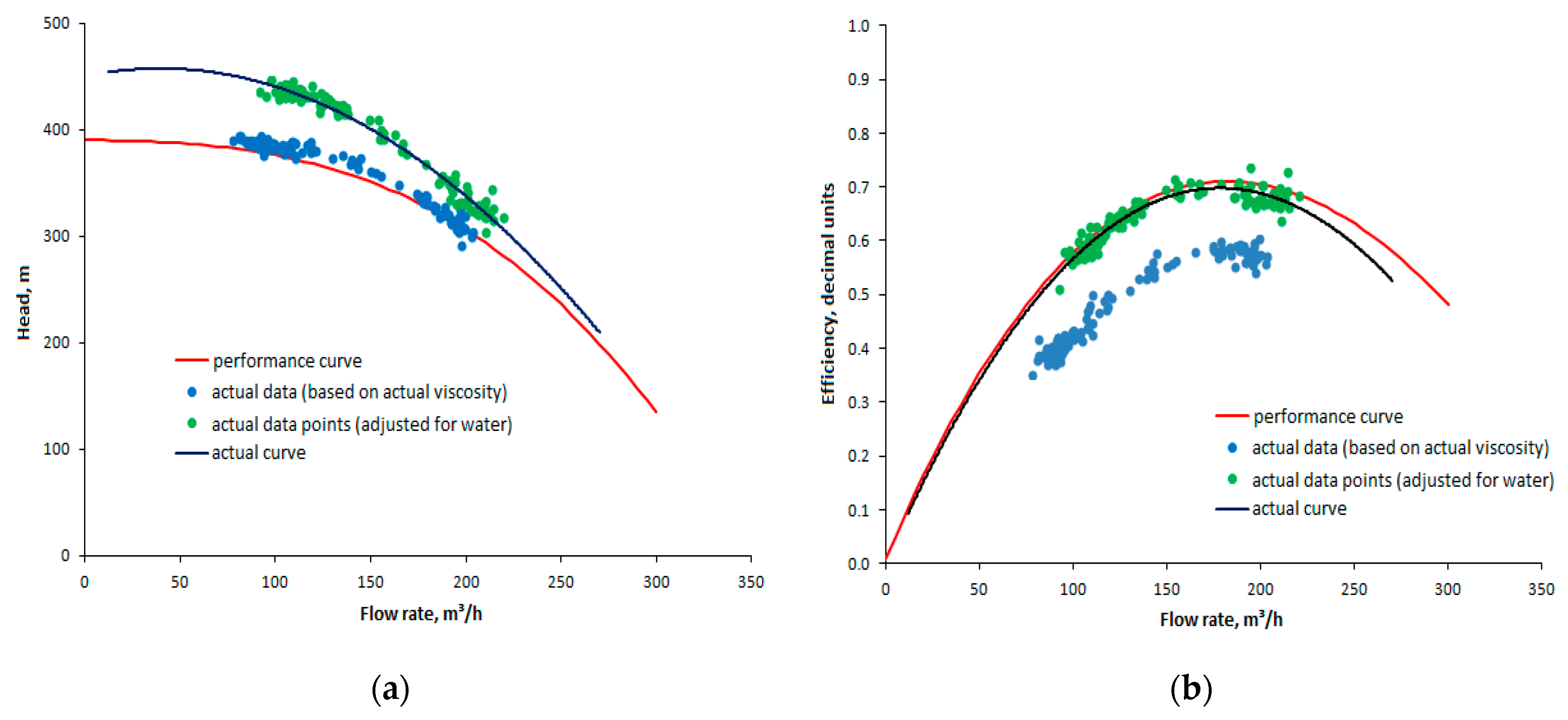
2.2.1. Digitalization of Equipment Characteristics at Stations

It is well established that pressure and pump efficiency are dependent on the flow rate of the pumped oil. Typically, this relationship is determined through factory testing and documented in the pump’s datasheet as pressure and efficiency characteristics. However, during operation, these characteristics tend to change over time. Using accurate sensor data, it is possible to establish a precise relationship between pressure and efficiency as a function of oil flow for each pump.

Figure 4 presents the actual pump characteristics at the Kassymov OPS derived from the data on flow rate, oil density, inlet and outlet pressure, and electricity consumption.

As can be seen from Figure 4, the actual pressure and efficiency values differ from the pump’s datasheet. The characteristics of the heating furnace are similarly digitized.

2.2.2. Digitalization of Hydraulic Parameters and Heat Transfer of the Pipeline

The oil flow mode in the Kassymov–Bolshoi Chagan main pipeline is turbulent. The Darcy–Weisbach formula [32] is used for the determination of hydraulic losses in pipelines. The hydraulic resistance coefficient of the Darcy–Weisbach formula, which depends on the Reynolds number and the pipe wall roughness, is determined using the empirical formulas of Nikuradze [32,33], Colebrook–White [34], and Altschul [35,36]. The article [36] compares the empirical formula proposed by Altschul [35] with experimental data collected from the SCADA systems of several main oil pipelines. The analysis reveals excellent agreement across all cases.

The pipe wall roughness coefficient changes during operation. Repairs and replacement of pipe sections can result in varying pipe roughness along the pipeline length. This means that the calculated hydraulic losses may significantly differ from the actual values if the pipeline’s real data are unavailable. By utilizing real-time data from the pressure and temperature sensors of the SCADA system, it is possible to develop a relationship for the hydraulic resistance coefficient of the pipe.

Figure 5 illustrates the relationship between the hydraulic resistance coefficient in the Darcy–Weisbach formula and the Reynolds number under turbulent flow conditions in the Kassymov–Bolshoi Chagan main pipeline.

The oil temperature in a pipe drops due to heat transfer with the surrounding soil; several formulas are available for the calculation of the heat transfer coefficient [37]. While some parameters, such as the flow velocity, oil and pipe material properties, insulation, and soil temperature, are known, the thermal conductivity of soil remains somewhat uncertain. Thermal conductivity can vary depending on the soil type and moisture content. As a result, the soil’s thermal conductivity is not constant along the pipeline or over time and is influenced by factors like snowmelt and rainfall frequency. Thus, the calculated oil temperature distributions along the pipeline could substantially differ from the actual measurements in the absence of actual data.

The soil’s thermal conductivity is adjusted to ensure that, for a specified flow rate, the initial oil and soil temperatures in the section and the predicted oil temperature at the section outlet closely align with the measured temperature. The thermal conductivity coefficient is averaged over the length and time. Length averaging depends on the temperature sensors’ density along the pipeline; they are typically spaced 5–15 km apart in the Kassymov–Bolshoi Chagan main pipeline. Time averaging generally covers a period of one month or 10–15 days, depending on the specific month.

Figure 6 compares the actual and predicted temperatures (represented by the red and green lines, respectively) at the section outlet, based on the determined coefficient of soil thermal conductivity in the Kassymov–Karmanovo linear section. The other parameters of the main pipeline are also compared with the experimental data.

3. SmartTranPro 1.7.1 Software

The numerical modeling of waxy oil hot pumping was carried out using the SmartTran Software [38,39]. The pressure and temperature calculations determine the accuracy of the digital twin results. The relationship between them can be derived from the motion and heat transfer equations.

3.1. System of Equations of Motion and Heat Transfer in the Pipeline’s Linear Part

A one-dimensional model can be considered due to the large length of the pipeline (about a thousand kilometers) compared to its inner diameter of 1 m.

The flow continuity equation is given by

$${\displaystyle \frac{\partial \rho }{\partial t}}+{\displaystyle \frac{\partial \rho u}{\partial x}}=0.$$

(1)

The equation for the momentum of turbulent flow can be written as

$$\rho {\displaystyle \frac{\partial u}{\partial t}}+{\displaystyle \frac{\partial P}{\partial x}}=-\zeta \left(\mathit{Re},\epsilon \right){\displaystyle \frac{\rho u\left|u\right|}{2D_1}}-\rho g\sin \beta \left(x\right).$$

(2)

The following equation describes the heat transfer of the flow to the environment:

$${\displaystyle \frac{\partial T}{\partial t}}+u{\displaystyle \frac{\partial T}{\partial x}}=-{\displaystyle \frac{4k}{\rho c_p{D}_1}}\left(T-T_w\right)+{\displaystyle \frac{\zeta u^3}{2c_p{D}_1}},$$

(3)

where p, u, and T are the pressure, flow velocity, and oil temperature (°C), respectively; $c_p$ is the heat capacity; $\zeta =\zeta \left(\mathit{Re},\epsilon \right)$ is the coefficient of hydraulic resistance; $\mathit{Re}=\rho uD/\mu$ is the Reynolds number; $k$ is the parameter of heat transfer with soil; $\epsilon$ is the parameter of roughness of tube walls; D₁ is the pipe diameter; T_w is the soil temperature; and $\beta =\beta \left(x\right)$ is the slope angle of the pipeline. Equation (3) describes the convective heat transfer (on the left), the heat exchange with the soil (the first term on the right), and the dissipation of kinetic energy into heat (the last term on the right).

The system of equations for motion and heat transfer (1)–(3) for an incompressible fluid with a constant flow rate can be written as [40]

$${\displaystyle \frac{\partial P}{\partial x}}=-\zeta {\displaystyle \frac{{\rho }_0{u}^2}{2D_1}}-{\rho }_{0}g\sin \beta \left(x\right),$$

(4)

$${\displaystyle \frac{\partial T}{\partial t}}+u{\displaystyle \frac{\partial T}{\partial x}}=-{\displaystyle \frac{4k}{{\rho }_0{c}_p{D}_1}}\left(T-T_w\right)+{\displaystyle \frac{\zeta u^3}{2c_p{D}_1}}.$$

(5)

The initial and boundary conditions are as follows:

$$T(x,0)=T_w\left(x\right), 0\le x\le L,$$

(6)

$$T(0,t)=T_0,\hspace{1em}\hspace{1em}P(0,t)=P_0, 0\le t\le T_s.$$

(7)

Equations (4) and (5) characterize the incompressible fluid flow with a quasi-steady pressure field and a time-varying temperature field. $P(x,t)$ and $T(x,t)$ are unknown variables. The flow velocity u and the flow rate Q are specified as constant values.

3.2. Closing Conditions

An empirical formula describes the dependence of oil viscosity on temperature:

$$\mu \left(T\right)=0.3585\cdot \mathit{exp}(-0.1792\cdot T),[\mathrm{P}\mathrm{a}\ast \mathrm{s}].$$

(8)

The hydraulic resistance coefficient $\zeta$ changes during the pipeline operation. The identification of this coefficient was given in Figure 5 by comparing it with the actual data.

$$\zeta \left(\mathit{Re},\epsilon \right)=0.1\cdot ({{\displaystyle \frac{68}{Re}} \epsilon )}^{0.25}.$$

(9)

The external coefficient of heat transfer with the soil ${\alpha }_2$ determines the heat transfer coefficient of the hot oil with the environment k. The Forchheimer–Graeber formula [41] determines this coefficient:

$$k={\alpha }_2{\displaystyle \frac{D_2}{D_1}}, {\alpha }_2={\displaystyle \frac{2{\lambda }_w}{D_2\mathit{ln}\left[\frac{2H}{D_2}+\sqrt{{\left(\frac{2H}{D_2}\right)}^2-1}\right]}},$$

(10)

where $D_2$ is the pipeline’s outer diameter; ${\lambda }_w$ is the thermal conductivity of the soil; and H is the pipeline’s depth in the soil.

The thermal conductivity coefficient of the soil, ${\lambda }_w$, depends on the soil type and its moisture content. Krego’s formula describes experimental data regarding the heat capacity of heavy oil:

$$c_p\left(T\right)={\displaystyle \frac{53357+107.2\cdot T}{\sqrt{{\rho }_0}}}, \left[{\displaystyle \frac{\mathrm{J}}{\mathrm{k}\mathrm{g}\ast \mathrm{℃}}}\right].$$

(11)

3.3. Optimization Criterion

The cost of “hot pumping” consists of two components: the cost of pumping and the cost of heating the oil. The pump consumes electrical energy, while the heating furnace uses gas fuel. Therefore, the total cost consists of the cost of the electrical energy consumed by the pumps and that of the fuel for the heater. If N is the pump’s power consumption and $z^e$ is the cost of electricity, then the cost of pumping is $z^{e}N$. If $z^f$ is the cost of fuel and $q^f$ is the fuel consumption rate of the heater, then the cost of heating is $z^f{q}^f$. For n stations, the optimal mode corresponds to the minimum of the total cost:

$${\sum }_{i=1}^n\left(z_i^e{\sum }_{j=1}^{m_i^p}{\delta }_{ij}^p{N}_{ij}\left(k_{ij}\right)+z_i^f{\sum }_{k=1}^{m_i^h}{\delta }_{ik}^h{q}_{ik}^f\right)\Rightarrow min,$$

(12)

where the upper indices p and ℎ refer to the pump and the heater, respectively; index i denotes the station number; $m_i^p$ is the number of pumps at the i-th station; $m_i^h$ is the number of heaters at the i-th station; $z_i^e$ is the cost of electricity (USD/(kW·h)); $z_i^f$ is the cost of fuel (USD/kg); $q_{ik}^f$ is the fuel consumption rate of the k-th heater at the i-th section (kg/h); $N_{ij}\left(k_{ij}\right)$ is the power consumption of the j-th pump at the i-th station (kW); and $k_{ij}$ is the ratio of the rotor speed of the pump to its nominal rotor speed.

Some pumps may operate or temporarily stop depending on the pressure field along the pipeline, and similarly, some heaters may stop or operate depending on the temperature field. The parameters ${\delta }_{ij}^p$ and ${\delta }_{ik}^h$ define their states. They are equal to 1 if the pump or heater is operating, and 0 otherwise.

The first term in Equation (12) defines the cost of the energy consumed by the pumps to create hydraulic pressure, and the second term defines the cost of fuel for heating the high-wax and high-viscosity oil at each station.

The functions $N_{ij}\left(k_{ij}\right)$ (power consumption) and $q_{ij}^f$ (fuel consumption rate) depend on the oil flow q through pressure and temperature and on the design combination of pump units and heating furnaces. Therefore, minimizing the functional (12) ensures the optimal value of q and the optimal design architecture of the pump-heating system.

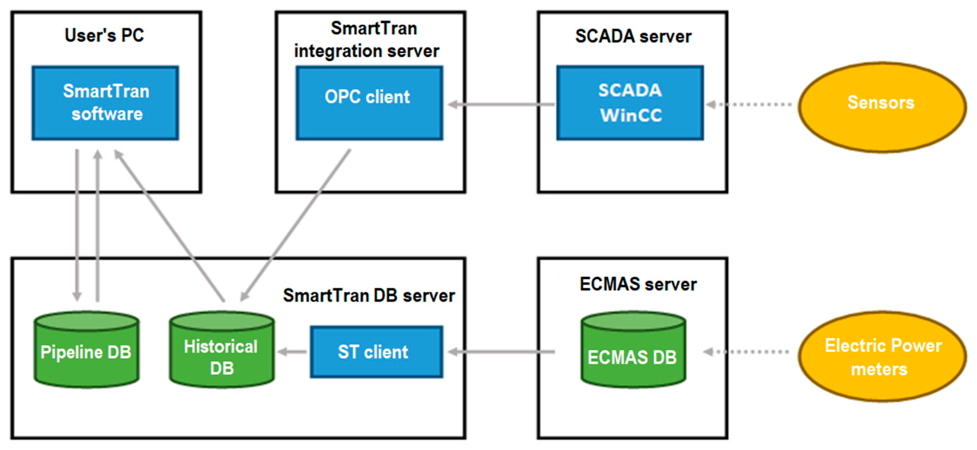
3.4. The Integration of SmartTran Software with SCADA and ECMAS

Figure 7 demonstrates how the SmartTran Software integrates with SCADA and ECMAS, incorporating data from sensors and electricity meters.

The data from the sensors (measurements of pressure, temperature, flow rate, network frequency, and electricity consumption) are sent to SCADA and ECMAS servers from all sections of the main pipeline. Every 30 min, a particular OPC client in the SmartTran Software receives sensor data from the SCADA and ECMAS servers via the WinCC system using the OPC protocol. The OPC client exports the received actual data to the SmartTran database server in the SmartTran Software database. Thus, the actual data of the technological pumping parameters are stored in the SmartTran Software database.

3.5. SmartTran Software Modules

The SmartTran Software has the following modules:

• Module for the thermal–hydraulic calculations of the stationary and non-stationary modes of waxy oil hot pumping;
• Module for identifying the pressure–volume characteristics and the efficiency of the pumping units depending on their service life;
• Module for identifying the efficiency of the heating furnaces depending on their service life;
• Module for identifying the hydraulic resistance of the pipelines, taking into account changes in pipe roughness;
• Module for identifying the thermal conductivity coefficient of the soil.

Integrating the SmartTran Software with SCADA and ECMAS allows for the acquisition of real-time data from the sensors and the use of the thermal–hydraulic modes of waxy oil hot pumping.

4. Discussion

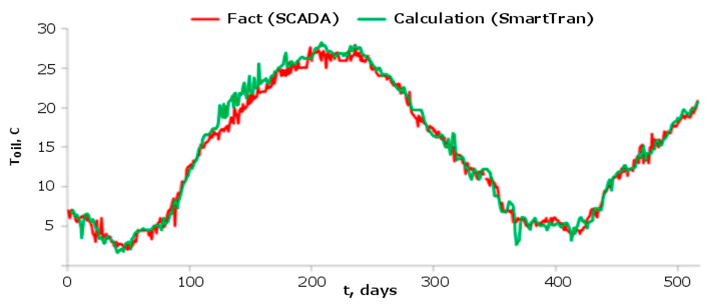
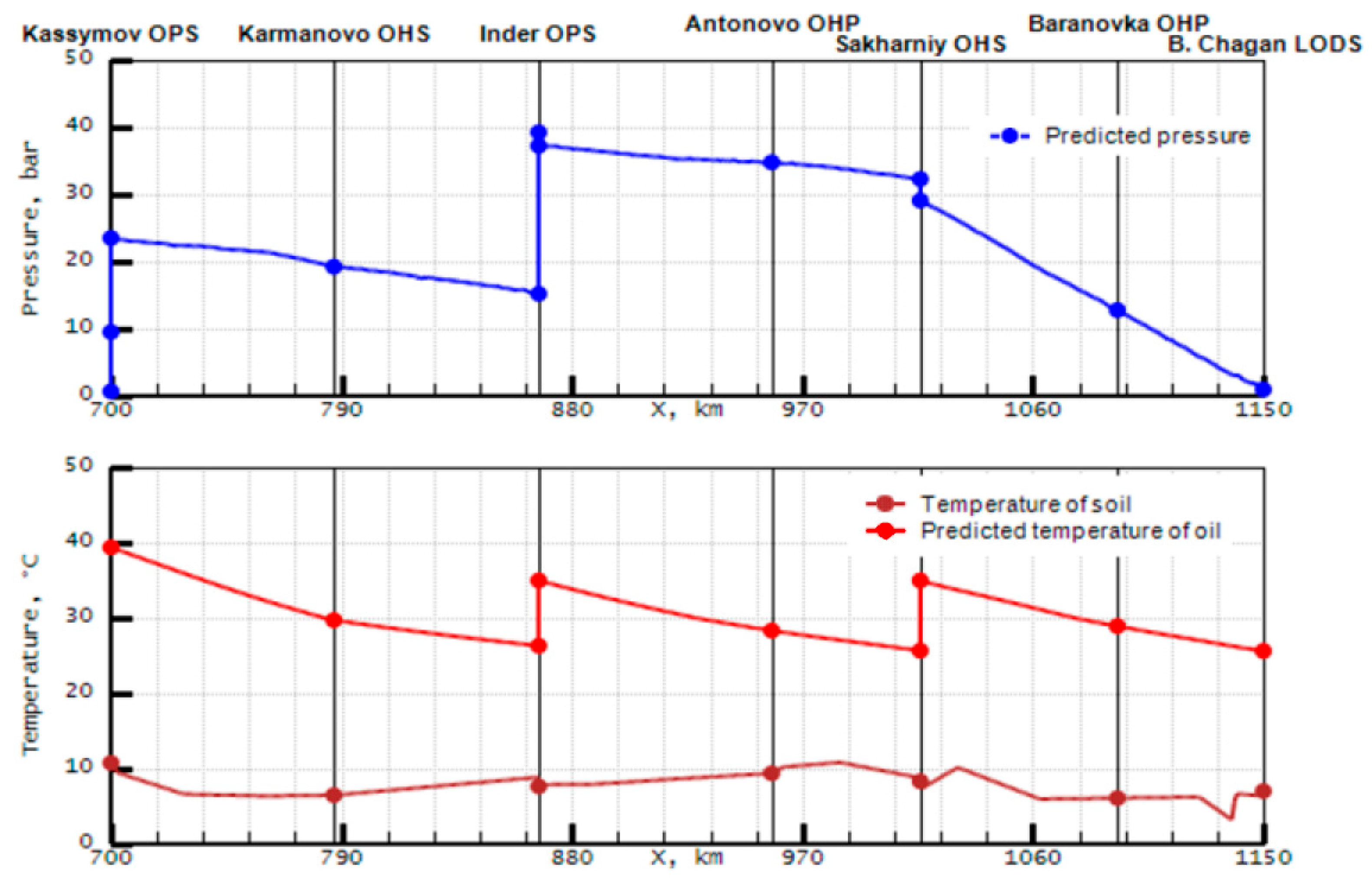
4.1. Calculated Pressure and Temperature Data

The calculations of waxy oil hot pumping are performed for the Kassymov–Bolshoi Chagan main pipeline (total length: L = 450 km). Kassymov and Inder are oil-pumping and oil-heating stations. Sakharniy is an oil-heating station. The pipeline’s inner diameter at Kassymov–Sakharniy is 1 m, and at Sakharniy–Bolshoi Chagan it is 0.7 m.

The sensors in SCADA receive the parameters of the hot pumping modes and serve as the input data for the calculations in the SmartTran Software.

Figure 8 shows the pressure (top graph) and temperature (bottom graph) distribution of waxy oil hot pumping along the Kassymov–Bolshoi Chagan main pipeline (predicted data are indicated as lines and real data of SCADA are shown as points). The flow rate is 1865 m³/h.

As shown in Figure 8, the pressure and temperature predicted by the SmartTran Software are consistent with the real data of SCADA. According to ECMAS, the operating pumps consume 4244 kW, or 2.79 kW*h/ton. The pumps consume USD 202.8/h, and the furnaces consume USD 129.39/h. The specific costs for pumping and heating are 0.133 USD/t and 0.085 USD/t, respectively.

4.2. Waxy Oil Heating Temperature Optimization

The optimization criterion (12) is used for performing the optimization calculations. The primary expense in hot pumping is waxy oil heating. Therefore, the optimization calculations are carried out to determine the effective heating temperature of the waxy oil. The calculations are performed at the same soil temperature and flow rate (1148 m³/h) in this section.

Figure 9 shows the pressure and temperature distributions based on the real data from SCADA.

The oil-heating temperature at the Kassymov station is 47 °C, at the Inder station it is 46 °C, and at the Sakharniy station it is 50 °C. These temperatures indicate a suboptimal operating mode.

Figure 10 shows the calculation results in the energy-saving mode. In this case, the oil temperature is assumed to remain above 28 °C, since waxy oil can exhibit non-Newtonian behavior below 28 °C, which would alter the calculation method.

The stepwise change in pressure at the Inder and Sakharniy stations means a pressure drop in the oil-heating furnaces. The optimal oil-heating temperatures at the Kassymov, Inder, and Sakharniy stations are 40 °C, 35 °C, and 30 °C, respectively. In the optimal operating mode, the total power of the pumping units is 3238 kW, whereas in the actual operating mode, it is 1515 kW. The total costs for oil pumping and heating are reduced from 321.1 USD/h to 265.3 USD/h, and the specific costs from 0.326 USD/t to 0.199 USD/t, representing a savings amount of up to 38.9% in the energy-saving mode.

5. Conclusions

The digital twin consists of correct initial data that ensures waxy oil hot pumping through the Kassymov–Bolshoi Chagan main pipeline. The parameters of the facilities and process equipment, the hydraulics and heat transfer, and the physical and chemical properties of oil are identified using actual data. The digital duplicates of the source data form the software base and make it possible to perform thermal–hydraulic calculations for waxy oil hot pumping. The SmartTran Software is integrated with SCADA and ECMAS to automate the calculations and optimize the technological modes of waxy oil hot pumping. The development originality lies in the fact that the SmartTran Software receives data from SCADA and ECMAS in real time and determines the energy-saving modes of waxy oil hot pumping.

References

1. Javaid, M.; Haleem, A.; Suman, R. Digital Twin applications toward Industry 4.0: A Review. Cogn. Robot. 2023, 3, 71–92. [Google Scholar] [CrossRef]
2. Aheleroff, S.; Zhong, R.Y.; Xu, X. A digital twin reference for mass personalization in industry 4.0. Procedia Cirp. 2020, 93, 228–233. [Google Scholar] [CrossRef]
3. Guerra-Zubiaga, D.; Kuts, V.; Mahmood, K.; Bondar, A.; Nasajpour-Esfahani, N.; Otto, T. An approach to develop a digital twin for industry 4.0 systems: Manufacturing automation case studies. Int. J. Comput. Integr. Manuf. 2021, 34, 933–949. [Google Scholar] [CrossRef]
4. Assawaarayakul, C.; Srisawat, W.; Ayuthaya, S.D.N.; Wattanasirichaigoon, S. Integrate digital twin to exist production system for industry 4.0. In Proceedings of the 4th Technology Innovation Management and Engineering Science International Conference (TIMES-iCON), Bangkok, Thailand, 11–13 December 2019. [Google Scholar] [CrossRef]
5. Uhlemann, T.H.J.; Lehmann, C.; Steinhilper, R. The digital twin: Realizing the cyber-physical production system for industry 4.0. Procedia Cirp. 2017, 61, 335–340. [Google Scholar] [CrossRef]
6. Qi, Q.; Tao, F. Digital twin and big data towards smart manufacturing and industry 4.0: 360 degree comparison. IEEE Access 2018, 6, 3585–3593. [Google Scholar] [CrossRef]
7. Vachálek, J.; Bartalský, L.; Rovný, O.; Šišmišová, D.; Morháč, M.; Lokšík, M. The digital twin of an industrial production line within the industry 4.0 concept. In Proceedings of the 21st International Conference on Process Control (PC), Strbske Pleso, Slovakia, 6–9 June 2017. [Google Scholar] [CrossRef]
8. Pires, F.; Cachada, A.; Barbosa, J.; Moreira, A.P.; Leitão, P. Digital twin in industry 4.0: Technologies, applications and challenges. In Proceedings of the 17th International Conference on Industrial Informatics (INDIN), Helsinki, Finland, 22–25 July 2019. [Google Scholar] [CrossRef]
9. Durão, L.F.; Haag, S.; Anderl, R.; Schützer, K.; Zancul, E. Digital twin requirements in the context of industry 4.0. In Proceedings of the IFIP International Conference on Product Lifecycle Management, Turin, Italy, 2–4 July 2018. [Google Scholar] [CrossRef]
10. Aheleroff, S.; Xu, X.; Zhong, R.Y.; Lu, Y. Digital twin as a service (DTaaS) in industry 4.0: An architecture reference model. Adv. Eng. Inform. 2021, 47, 101225. [Google Scholar] [CrossRef]
11. Nguyen, H.X.; Trestian, R.; To, D.; Tatipamula, M. Digital twin for 5G and beyond. IEEE Commun. Mag. 2021, 59, 10–15. [Google Scholar] [CrossRef]
12. Agnusdei, G.P.; Elia, V.; Gnoni, M.G. Is digital twin technology supporting safety management? A bibliometric and systematic review. Appl. Sci. 2021, 11, 2767. [Google Scholar] [CrossRef]
13. Qazi, A.M.; Mahmood, S.H.; Haleem, A.; Bahl, S.; Javaid, M.; Gopal, K. The impact of smart materials, digital twins (DTs) and Internet of things (IoT) in an Industry 4.0 integrated automation industry. Mater. Today Proc. 2022, 6, 18–25. [Google Scholar] [CrossRef]
14. Fuller, A.; Fan, Z.; Day, C.; Barlow, C. Digital twin: Enabling technologies, challenges and open research. IEEE Access 2020, 8, 108952–108971. [Google Scholar] [CrossRef]
15. Martínez-Gutiérrez, A.; Díez-González, J.; Ferrero-Guillén, R.; Verde, P.; Álvarez, R.; Perez, H. Digital twin for automatic transportation in industry 4.0. Sensors 2021, 21, 3344. [Google Scholar] [CrossRef] [PubMed]
16. Hinduja, H.; Kekkar, S.; Chourasia, S.; Chakrapani, H.B. Industry 4.0: Digital twin and its industrial applications. Int. J. Eng. Sci. Tech. 2020, 8, 1–7. [Google Scholar]
17. Rolle, R.; Martucci, V.; Godoy, E. Architecture for Digital Twin implementation focusing on Industry 4.0. IEEE Lat. Am. Tran. 2020, 18, 889–898. [Google Scholar] [CrossRef]
18. Barykin, S.Y.; Bochkarev, A.A.; Kalinina, O.V.; Yadykin, V.K. Concept for a supply chain digital twin. Int. J. Math. Eng. Manag. Sci. 2020, 5, 1498–1515. [Google Scholar] [CrossRef]
19. Židek, K.; Piteľ, J.; Adámek, M.; Lazorík, P.; Hošovský, A. Digital twin of experimental smart manufacturing assembly system for industry 4.0 concept. Sustainability 2020, 12, 3658. [Google Scholar] [CrossRef]
20. Kholopov, V.A.; Antonov, S.V.; Kashirskaya, E.N. Application of the digital twin concept to solve the monitoring task of machine-building technological process. In Proceedings of the International Russian Automation Conference (RusAutoCon), Sochi, Russia, 8–14 September 2019. [Google Scholar] [CrossRef]
21. Papacharalampopoulos, A.; Stavropoulos, P.; Petrides, D. Towards a digital twin for manufacturing processes: Applicability on laser welding. Procedia Cirp. 2020, 88, 110–115. [Google Scholar] [CrossRef]
22. Sajid, S.; Haleem, A.; Bahl, S.; Javaid, M.; Goyal, T.; Mittal, M. Data science applications for predictive maintenance and materials science in context to Industry 4.0. Mater. Today Proc. 2021, 45, 4898–4905. [Google Scholar] [CrossRef]
23. Hearn, M.; Rix, S. Cybersecurity considerations for digital twin implementations. IIC J. Innov. 2019, 10, 107–113. [Google Scholar]
24. Lee, J.; Azamfar, M.; Singh, J.; Siahpour, S. Integration of digital twin and deep learning in cyber-physical systems: Towards smart manufacturing. IET Coll. Intel. Manuf. 2020, 2, 34–36. [Google Scholar] [CrossRef]
25. Jiang, Z.; Guo, Y.; Wang, Z. Digital twin to improve the virtual-real integration of industrial IoT. J. Ind. Inf. Integr. 2021, 22, 100196. [Google Scholar] [CrossRef]
26. Negri, E.; Fumagalli, L.; Cimino, C.; Macchi, M. FMU-supported simulation for CPS digital twin. Procedia manuf. 2019, 28, 201–206. [Google Scholar] [CrossRef]
27. Tao, F.; Zhang, M. Digital twin shop-floor: A new shop-floor paradigm towards smart manufacturing. IEEE Access 2017, 5, 20418–20427. [Google Scholar] [CrossRef]
28. Negri, E.; Fumagalli, L.; Macchi, M. A review of the roles of digital twin in CPS-based production systems. Procedia Manuf. 2017, 11, 939–948. [Google Scholar] [CrossRef]
29. Pang, T.Y.; Pelaez Restrepo, J.D.; Cheng, C.T.; Yasin, A.; Lim, H.; Miletic, M. Developing a digital twin and digital thread framework for an ‘Industry 4.0’ Shipyard. Appl. Sci. 2021, 11, 1097. [Google Scholar] [CrossRef]
30. Schroeder, G.N.; Steinmetz, C.; Rodrigues, R.N.; Henriques, R.V.B.; Rettberg, A.; Pereira, C.E. A methodology for digital twin modeling and deployment for industry 4.0. Proc. IEEE 2020, 109, 556–567. [Google Scholar] [CrossRef]
31. Priyanka, E.B.; Thangavel, S.; Gao, X. Review analysis on cloud computing based smart grid technology in the oil pipeline sensor network system. Pet. Res. 2021, 6, 77–90. [Google Scholar] [CrossRef]
32. Nikuradse, J. Regularity of turbulent flow in smooth pipes. In Problem of Turbulence; ONTI NKTP SSSR: Moscow, Russia; Saint Petersburg, Russia, 1936; pp. 75–150. (In Russian) [Google Scholar]
33. Schlikhting, G. Theory of Boundary-Layer; Nauka: Moscow, Russia, 1974. (In Russian) [Google Scholar]
34. Colebrook, C.F.; White, C.M. Experiments with fluid friction in roughened pipes. Proc. R. Soc. Lond. Ser. A Math. Phys. Sci. 1937, 161, 367–381. [Google Scholar] [CrossRef]
35. Altshul, A.D. Hydraulic Resistance; Nedra: Moscow, Russia, 1982. (In Russian) [Google Scholar]
36. Bekibayev, T.; Zhapbasbayev, U.; Ramazanova, G.; Bossinov, D.; Pham, D.T. Oil pipeline hydraulic resistance coefficient identification. Cogent Eng. 2021, 8, 1950303. [Google Scholar] [CrossRef]
37. Kondratev, A.S.; Nha, T.L.; Shvydko, P.P. The Colebrook-White general formulas pipe flow for arbitrary sand roughnees of pipe wall. Fundam. Res. 2017, 1, 74–78. [Google Scholar]
38. Bekibayev, T.T.; Ramazanova, G.I.; Pakhomov, M.A. The problem of optimizing pumping units for oil transportation. Compl. Use of Min. Resour. 2022, 321, 38–46. [Google Scholar] [CrossRef]
39. Beysembetov, I.K.; Bekibayev, T.T.; Zhapbasbayev, U.K.; Ramazanova, G.I.; Panfilov, M. SmartTran Software for transportation of oil JSC KazTransOil. News NAS RK. Ser. Geol. Tech. Sci. 2020, 2, 6–13. [Google Scholar] [CrossRef]
40. Bekibayev, T.T.; Zhapbasbayev, U.K.; Ramazanova, G.I. Optimal regimes of heavy oil transportation through a heated pipeline. J. Process Control. 2022, 115, 27–35. [Google Scholar] [CrossRef]
41. Garris, N.A.; Rusakov, A.I.; Baykova, L.R. New approach to estimation of thermal conductivity coefficient for underground pipeline forming a thawing halo in permafrost. J. Phys. 2018, 1111, 012016. [Google Scholar] [CrossRef]
Figure 1. Digital twin structure.
Energies 18 00202 g001
Figure 2. Scheme of the Kassymov–Bolshoi Chagan main pipeline.
Energies 18 00202 g002
Figure 3. Digital profile of the Kassymov–Bolshoi Chagan main pipeline.
Energies 18 00202 g003
Figure 4. Digitalization of pump characteristics at the Kassymov station: (a) pressure characteristic graph; (b) efficiency graph.
Energies 18 00202 g004
Figure 5. Identification of the hydraulic resistance coefficient in the Kassymov–Bolshoi Chagan main pipeline.
Energies 18 00202 g005
Figure 6. Actual and predicted oil temperatures at the section outlet of the Kassymov–Karmanovo section.
Energies 18 00202 g006
Figure 7. Scheme of interaction between SmartTran Software and SCADA and ECMAS.
Energies 18 00202 g007
Figure 8. Pressure and temperature distribution of waxy oil hot pumping along the Kassymov–Bolshoi Chagan main pipeline.
Energies 18 00202 g008
Figure 9. Pressure and temperature distribution along the Kassymov–Bolshoi Chagan main pipeline according to SCADA.
Energies 18 00202 g009
Figure 10. Pressure and temperature distributions along the Kassymov–Bolshoi Chagan main pipeline in energy-saving mode.
Energies 18 00202 g010
Disclaimer/Publisher’s Note: The statements, opinions and data contained in all publications are solely those of the individual author(s) and contributor(s) and not of MDPI and/or the editor(s). MDPI and/or the editor(s) disclaim responsibility for any injury to people or property resulting from any ideas, methods, instructions or products referred to in the content.