PV Cells and Modules Parameter Estimation Using Coati Optimization Algorithm

Abstract

In recent times, there have been notable advancements in solar energy and other renewable sources, underscoring their vital contribution to environmental conservation. Solar cells play a crucial role in converting sunlight into electricity, providing a sustainable energy alternative. Despite their significance, effectively optimizing photovoltaic system parameters remains a challenge. To tackle this issue, this study introduces a new optimization approach based on the coati optimization algorithm (COA), which integrates opposition-based learning and chaos theory. Unlike existing methods, the COA aims to maximize power output by integrating solar system parameters efficiently. This strategy represents a significant improvement over traditional algorithms, as evidenced by experimental findings demonstrating improved parameter setting accuracy and a substantial increase in the Friedman rating. As global energy demand continues to rise due to industrial expansion and population growth, the importance of sustainable energy sources becomes increasingly evident. Solar energy, characterized by its renewable nature, presents a promising solution to combat environmental pollution and lessen dependence on fossil fuels. This research emphasizes the critical role of COA-based optimization in advancing solar energy utilization and underscores the necessity for ongoing development in this field.

1. Introduction

In recent years, the increase in energy demand has caused environmental concerns to increase. Although fossil fuels are relatively cheap, they are a continuous source of global warming and air pollution. Oil and gas extraction provide energy resources, but they have become the main factor for environmental pollution in the past decades. Furthermore, estimates show that energy sources such as oil and gas will run out in the coming years, so finding new and renewable energy sources is vital [1,2].

In recent years, clean and renewable energies have developed and progressed, so now, they are a suitable alternative to fossil fuels (oil and gas). Renewable energy, such as the power obtained from the sun, wind, tides, water, hot springs, etc., has been attracting the attention of scientists. Among renewable energies, solar energy is more accessible than other energies and used in most areas of the earth. Solar energy is a renewable energy source. Unlike electricity generation by fossil fuels such as gas and oil, solar energy does not cause any environmental pollution [3]. Estimates show that the share of solar energy in electricity production will reach about USD 194 billion by 2027, which shows the importance of this energy [4]. Photovoltaic systems help transform solar energy into valuable electricity. Photovoltaic (PV) systems convert solar energy into electricity using semiconductor technology [5]. Progress in renewable energy has influenced many countries and governments to use this clean energy to produce electricity. Solar energy is an economical and abundant clean energy source. Due to the easy access to sunlight, solar systems are used in many countries in Africa, the Middle East, and America [6].

Solar energy conversion into electricity in solar cells needs devices based on electronic semiconductors with a thin layer. A solar system based on semiconductor crystals is usually made of two types: multi-crystalline [7] and monocrystalline [8] solar modules. Single-crystal semiconductors are more efficient for generating power and have better electrical properties. However, despite having a large production capacity, monocrystalline PV modules are unprofitable because of the high cost of the crystalline wafer-based technology. An alternate process to single-crystal modules for solar power production is thin film technology. This method typically uses amorphous silicon [8] or other semiconductor materials such as gallium arsenide [9], copper indium gallium selenide [10], or cadmium telluride [11].

Solar energy is a clean, renewable source because it directly converts solar energy into electricity using semiconductor technology in photovoltaic devices. The amount of energy production from PV systems depends on weather conditions, solar radiation, ambient temperature, type of modules, etc. [11].

An accurate understanding of PV’s electrical structure and modules may help researchers increase power production efficiency. PV systems comprise a power converter, a solar generator, and other parts connected to the power grid by control circuits, power converters, or inverters. The production efficiency of PV devices must be increased through effective design and implementation. PV power generation is non-linear by nature and is impacted by environmental variables, including temperature, light intensity, and load characteristics. Therefore, PV devices need control circuits for high power-generation performance. Control circuits in PV devices optimize current and output voltage to increase power production and system efficiency [10].

The two main models for modeling solar PV cells include the double-diode model (DDM) [12] and the single-diode model (SDM) [13]. DDM can effectively represent a PV cell since it is more accurate than SDM. Planning and optimizing solar PV cells is complicated because there are about ten unknown variables in this problem [9]. Investigations show that current curves in terms of voltage or I-V in PV cells have a non-linear and complex nature. A controller is an essential component in any PV circuit. In photovoltaic systems, controllers are usually used to manage the charging of batteries or the power supplies to the grid [14]. Maximum power point tracking (MPPT) is one of the capabilities that some controllers use to increase solar cells’ power efficiency. MPPT algorithms, especially in large systems, are essential in increasing power production and management. For a solar module, the MPPT tracks the current and voltage to reach the maximum power and then absorbs it [14]. There are three ways to find MPPT when solving non-linear equations in a controller. Numerical approaches [10], evolutionary algorithms [15], and analytical methods [16] are a few of these techniques. In order to solve non-linear calculations with numerous unknowns, the first method, which mostly uses linear calculations, must be initiated. Predicting the initial value for solving the equation, which determines the convergence rate of the solution, is the most difficult aspect of such approaches. The second approach relies on local search techniques. Although numerical approaches have several limitations, they can generate properties of PV cells that are more precise than analytical methods. First, the convergence of this technique heavily depends on the initial explanation. Second, they are prone to errors, and third, obtaining the appropriate model parameters takes time and effort. In recent years, optimization and meta-heuristic methods have played an essential role in solving non-linear calculations and providing solutions very close to the optimal solution. Using these techniques, searching for the ideal solution takes little time. Various meta-heuristic techniques have recently been employed to pinpoint solar cell model parameters in PV systems; for example, GA [13], PSO, MCDM [12], WOA [17], GWO [18], and IHHO-VMD [16] algorithms are used for this purpose. Table 1 presents the application of meta-heuristic, bio-inspired, and hybrid optimization algorithms for parameter extraction of PV cell models.

Table 1. Utilizing meta-heuristic optimization algorithms for parameter extraction of PV cell models.

Ref	Aim	Algorithm	Limitations	Advantages	Results
[10,13]	The study seeks to create a method for designing zero-energy residential structures by employing building performance simulation technology and multi-objective optimization, aiming to attain the most efficient energy-saving solutions adaptable to various climate zones in China.	NSGA-II	Challenges entail the necessity for enhancing the building energy calculation model to encompass regional nuances and the simplification of some parameters for research practicality.	The strengths of the research include the creation of a parametric design platform to determine energy consumption thresholds and photovoltaic replacement rates specific to diverse climate zones, providing valuable guidance for policymakers and standard-setting bodies. Furthermore, the study underscores the significance of holistic considerations beyond mere energy usage in residential architectural planning.	The findings indicate that near-zero energy consumption is viable in select climate zones in China, with defined photovoltaic replacement rates. Additionally, the research offers crucial guidance on fine-tuning design parameters to harmonize energy efficiency, economic viability, and residential comfort, highlighting the need to avoid overly zealous pursuit of zero-energy targets to maintain a balanced approach.
[12]	The study aims to compare decision tree and particle swarm optimization algorithms for identifying optimal solar power plant locations, providing insights for renewable energy planning in Iran.	PSO, MCDM	The research recognizes constraints such as the unavailability of specific data such as transmission line information, potentially impacting the precision of the findings.	The article presents the application of the decision tree method in identifying prime sites for solar power plants, offering a fresh approach to environmental studies. Furthermore, it assesses the efficacy of the decision tree against the PSO method, emphasizing the decision tree’s advantage in this particular domain.	The decision tree method outperforms PSO in predicting high-potential solar energy areas, emphasizing its effectiveness in identifying optimal sites for solar projects. Employing spatial data mining techniques is advised to improve site suitability assessment for power plants, with eastern and southeastern Iran highlighted as especially favorable regions.
[17]	The study investigates the impact of PVs and EVs on economic emission dispatch, proposes a modified WOA for optimization, and verifies its performance with simulations.	WOA	Constraints of the study encompass the intricate nature of the optimization issue, non-linear and non-convex constraints, and the necessity for meticulous consideration of diverse factors like valve point loading effects, restricted areas, and transmission losses.	The strengths of the study are found in its capacity to efficiently handle the intricate and contradictory aims of economic emission dispatching through the integration of PVs and EVs, along with proposing a customized WOA algorithm that surpasses other optimization methods in delivering superior quality results.	The findings of the study indicate that incorporating PVs and EVs into economic dispatching leads to lower emissions and energy generation costs, while the proposed modified WOA algorithm consistently yields superior quality results when compared to other optimization algorithms employed for economic load dispatch.
[18]	The research aims to improve the performance of MPPT controllers by optimizing them with the GWO algorithm and assessing their efficiency compared to traditional methods in various conditions, focusing on response time, efficiency, and power generation.	GWO	Challenges in the study encompass the need for fine-tuning the metaheuristic algorithm when applied within a PLC mandating historical irradiation data across diverse weather conditions.	The strengths of the study are evident in the enhanced efficacy of the MPPT controller, optimized using the GWO algorithm, resulting in superior efficiency and power generation when contrasted with conventional approaches. Furthermore, the research offers valuable observations regarding the response time of various algorithms amidst changing conditions.	The research demonstrates that optimizing the MPPT controller with GWO enhances efficiency and power generation while minimizing overshooting, with GWO exhibiting faster response times than traditional algorithms.
[16]	The research aims to mitigate the variability in photovoltaic output by suggesting a hybrid energy storage setup strategy.	IHHO-VMD	Challenges involve the possibility of constraining photovoltaic output and diminishing power generation, alongside the restricted energy storage capacity of the HESS, indicating the need for exploring improved decomposition techniques and integrating electric hydrogen into HESS, warranting further investigation.	Benefits encompass a 6.15% decrease in the hybrid energy storage system cost relative to the original algorithm as well as mitigated power fluctuations, leading to enhanced system economy and stability.	The IHHO-VMD algorithm effectively reduces energy storage system costs, enhances power allocation, and stabilizes photovoltaic grid-connected power. While MA helps mitigate power fluctuations, challenges remain with photovoltaic output and HESS capacity, warranting further exploration of improved decomposition methods and HESS expansion.

Finding appropriate model parameters is a challenging optimization problem for evaluating PV parameters. In general, classical optimization algorithms cannot find the optimal solution. New meta-heuristic algorithms have demonstrated better ability in global and local search and search the problem space more optimally. Optimization methods such as genetics and particles use basic mechanisms for searching, while optimizing the parameters of a PV is a complex problem with several variables. In this research, we undertook parameter optimization for the SDM, DDM, and PV solar cell models to enhance solar cell efficiency. We thus propose a tailored COA [19], specifically crafted to improve the efficiency of PV devices. Moreover, we introduce an enhanced version of the COA that fosters mutual learning. Additionally, we conducted parameter estimation for PV models, comparing them with recent meta-heuristic methods. Finally, we herein present an upgraded iteration of the coati optimization algorithm, which integrates chaos theory, to provide a comprehensive approach to optimizing solar cell parameters and improving efficiency. This study introduces a novel optimization strategy aimed at enhancing the efficiency of solar cells and optimizing their parameters. The main contributions of this manuscript are as follows:

▪

Parameter optimization for the SDM, DDM, and PV solar cell models;

▪

Improving the efficiency of solar cells;

▪

Introducing a coati optimization algorithm [15] designed to enhance the efficiency of PV devices;

▪

Introducing an upgraded version of the coati optimization algorithm that fosters mutual learning;

▪

Estimating parameters for PV models and comparing them with recent meta-heuristic methods;

▪

Introducing an enhanced version of the coati optimization algorithm integrated with chaos theory.

This research work was compiled and is herein presented in five sections. Section 2 introduces solar cells and their components and related works for optimizing PV device parameters review. Section 3 shows the proposed method for improving the COA or the PV parameters’ optimal estimation. Section 4 explains tests and implementation, and the results are analyzed and evaluated. Finally, Section 5 includes the conclusions and future work.

2. Related Works

A strategy for optimizing the photovoltaic model’s parameters was presented in research [20] that applied northern goshawk optimization (NGO). In order to determine the triple-diode model’s parameters (PV module), this research applied an optimization algorithm known as NGO. Three commercial PV modules were applied in the current research. The simulation results demonstrate that NGO outperformed the other optimization algorithms in terms of speed and accuracy. Furthermore, with this technique, the cost function for the Canadian Solar CS6K-M module may be reduced to 0.000195.

A strategy for optimizing the solar photovoltaic models’ parameters by applying differential evolution and queue search optimization was discussed in another paper [21]. The PV model has a multi-model and non-linear specification, making it challenging to determine its ideal values. The algorithms employed to address this problem are prone to stick in local optima because of the non-linear nature of the problem. Due to their large impact on the PV system’s current and power generation performance, the parameters’ appropriate estimation is crucial. In order to extract the ideal PV parameter values, this study provided an enhanced queue search optimization (QSO) based on the differential evolution (DE) method. Their method outperformed other methods like genetic algorithms and particles for obtaining the best parameters, e.g., single-diode, double-diode, and PV module models.

A previous study introduced a fuzzy solar PV and wind turbine system employing particle swarm optimization (PSO) [22] to boost efficiency. However, accurately creating a power forecasting model allows a researcher to regulate the randomized behavior of solar and wind energy sources. Solar PV and wind forecasting algorithms based on fuzzy logic may better handle this unpredictable and random aspect. Furthermore, the performance of the forecasting model was improved by using hybrid fuzzy–PSO intelligent forecasting, which also enhanced the system’s restrictions. Their tests revealed that the proposed fuzzy model was more effective in boosting the power of solar and wind systems than the fuzzy model used in conjunction with a genetic algorithm (GA). In another study [23], the optimization of electricity production by solar energy was presented using improved MPPT techniques. In this research, they optimized the parameters of the photovoltaic module with optimization methods.

In a research paper [24], a hybrid approach based on the bat algorithms (BA) and grasshopper optimization algorithms (GOA) was presented to maximize power generation through solar photovoltaics. This research used a combined meta-heuristic algorithm to extract the maximum power from PV using the XSG controller.

The proposed algorithm performed well for power extraction, according to experiments, and is more capable and effective at boosting power than the BA and GOA algorithms.

One paper [25] validated the firefly algorithm’s efficacy in optimizing solar cell and photovoltaic module parameters, especially compared to experimental data and the existing literature, highlighting its effectiveness in minimizing error metrics and accurately reproducing current-voltage characteristics under varying irradiance and temperature conditions.

The research from [26] endeavored to create a dependable approach employing the Lambert W function to precisely estimate single-diode PV parameters, tackling issues present in current methodologies, such as inaccuracies in RMSE computation and excessive dependence on optimization methods. The suggested analytical solution enhanced parameter estimation accuracy, notably observable in single-diode PV equivalent circuits, by rectifying RMSE calculation inaccuracies identified in the existing literature.

The study endeavored to develop a dependable method for accurately estimating PV parameters, utilizing an innovative hybrid strategy that integrates diversification and intensification mechanisms from different metaheuristics (MHs). It tackled issues such as computational complexity and parameter sensitivity, highlighting its ability to adapt to various optimization challenges, explore multiple search spaces simultaneously, and enhance accuracy and reliability as evidenced by comparisons with alternative MHs and benchmark functions [27].

The reference [19] presented the arithmetic optimization algorithm (IAOA) as a solution to improve the estimation of PV model parameters, tackling issues such as parameter sensitivity and computational complexity. Despite its potential drawbacks, IAOA showcased notable precision and dependability in estimating solar cell parameters, efficiently optimizing PV models across various scenarios and surpassing other algorithms in terms of accuracy and performance.

The study of [28] presented and assessed the mountain gazelle optimizer (MGO) algorithm’s effectiveness in pinpointing PV model parameters, specifically targeting the SDM and DDM of photovoltaic systems. MGO showcased benefits like rapid processing, consistent convergence, and precise results, outperforming other algorithms with the lowest RMSE across 30 separate iterations.

The use of the new optimization technique to predict the ideal parameters in solar modules was observed in one study [29]. This study considered the Harris hawks optimizer (HHO) to acquire the PV systems’ model parameters. The modified HHO offers a worldwide search capacity, high efficiency, and high convergence speed compared to the conventional method. In addition, the research revealed that the HHO method has a lower error value for voltage power (P-V) and current-voltage (I-V) features.

Another research [30] presented the evaluation and improvement of the photovoltaic grid-connected system using the VPFOTADF controller with the improved version of Wall’s algorithm. This paper aimed to design solar cells to reduce harmonic distortion and improve the solar system’s performance connected to the photovoltaic grid using group intelligence. The solar PV system has components such as a booster converter, photovoltaic array, multi-level inverter, and controller. This study optimized the amplifier converter using the improved WOA algorithm. Evaluation and tests showed that their method increases the production capacity more than the WOA algorithm.

In another study, an improved arithmetic optimization algorithm (AOA) was proposed for extracting parameters of a single-diode photovoltaic solar cell model [31]. The experimental findings demonstrated that IAOA outcomes are more effective and accurate than those obtained using AOA.

A method to determine the solar PV model’s optimal parameters using the chimp optimization algorithm (ChOA) was mentioned in one research paper [21]. To produce precise and trustworthy PV models, including single-diode, dual-diode, triple-diode, and PV module models, this research suggested a novel technique called ChOA that is inspired by nature. The fundamental difficulty in predicting the PV models’ parameters using optimization methods is convergence to the local optimum. Therefore, this study integrated the best distinctive aspects of PSO and a local search technique. The tests revealed that their suggested algorithm outperforms the EHHOA, BMO, FPSO, CBBO, and GOTLA algorithms in terms of optimizing the three commercial modules’ parameters that are often used: KC200GT, SW255, and SM55 multi-crystal.

3. Methodology

In the present study, the COA algorithm was selected due to its pioneering methodology, which amalgamates elements of biological inspiration, population-based optimization, modeling of natural behaviors, mutual learning, opposition-based learning, and integration of chaos theory. This comprehensive approach empowers the algorithm to effectively navigate intricate search spaces and discover high-quality solutions, rendering it a compelling option for optimizing PV system parameters. The benefits of utilizing the COA for optimizing PV systems are outlined in Table 2.

Table 2. Advantages of the COA for PV System Optimization.

Ref	Advantage	Description	Benefit for PV System Optimization
[32]	Biological inspiration	Mimics coatis’ intelligent hunting and evasion behaviors.	Novel optimization perspective, potentially leading to adaptive and resourceful solutions.
[15]	Population-based approach	Explores multiple solutions simultaneously.	Efficiently finds global optimums in complex PV system problems.
[33]	Integration of natural behaviors	Models coatis’ hunting and evasion behaviors for optimization.	Achieves faster convergence and more robust solutions.
[34]	Opposition-based Learning	Diversifies exploration by generating opposite solutions.	Prevents premature convergence and encourages exploration of diverse regions.
[35]	Chaos theory integration	Introduces randomness to escape local optima.	Enhances exploration capabilities and avoids stagnation.

The P-V and I-V curve properties of PV modules and solar cells are created using two common mathematical models described in this section. First, the SDM model and formulation are explained, then the DDM model is explained, and finally, the circuit’s optimum parameters are discovered using the coati optimization algorithm.

3.1. SMD Circuit

Figure 1 shows the electrical circuit equivalent to SDM. In this circuit, I_ph represents the current produced by the photogenerated current. The SDM framework is relatively simple. First, the generated diode current I_d, output current I_L, shunt current I_sh, and hot I_ph are defined.

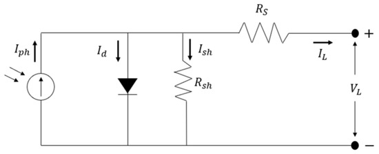
Figure 1. SDM circuit structure in PV systems [36].

Then, Kirchhoff’s current law is used to obtain I_L using Equation (1). The equations of the diode Shockley and Ohm laws are, respectively, used to obtain I_d using Equation (2) and $I_{sh}$ applying Equation (3).

$$I_L=I_{ph}-I_d-I_{sh}$$

(1)

$$I_d=I_{sd}\cdot \left[\exp \left(\frac{q\cdot \left(V_L+R_S\cdot I_L\right)}{n\cdot k\cdot T}\right)-1\right]$$

(2)

$$I_{sh}=\frac{V_L+R_S\cdot I_L}{R_{sh}}$$

(3)

Equation (1) is expanded using Equations (2)–(4):

$$I_L=I_{ph}-I_d\cdot \left[\exp \left(\frac{q\cdot \left(V_L+R_S\cdot I_L\right)}{n\cdot k\cdot T}\right)-1\right]-\frac{V_L+R_S\cdot I_L}{R_{sh}}$$

(4)

R_S is a series resistor, R_sh is a parallel resistor, V_L stands for output voltage k, q stands for initial charge (1.60217646 × 10⁻¹⁹), and n is the ideality factor of the diode and refers to Boltzmann’s constant and equals (1.3806503 × 10⁻²³ J/K q). Here, SDM identifies five different unknown parameters ($I_{ph}$, $I_d$, $R_S$, $R_{sh}$, and n), and T represents the absolute temperature.

3.2. DDM Circuit

The corresponding electrical circuit for DDM is shown in Figure 2. DDM can more precisely depict the voltage–current relationship given the inherent limitations of SDM. A diagram of the DDM circuit is shown in Figure 2. Because DDM has an additional diode (in parallel) compared to SDM, Figure 2 demonstrates how DDM differs from SDM. I_L is calculated using Equation (5):

$$I_L=I_{ph}-I_{d1}\cdot \left[\exp \left(\frac{q\cdot \left(V_L+R_S\cdot I_L\right)}{n_1\cdot k\cdot T}\right)-1\right]-I_{d2}\cdot \left[\exp \left(\frac{q\cdot \left(V_L+R_S\cdot I_L\right)}{n_2\cdot k\cdot T}\right)-1\right]-\frac{V_L+R_S\cdot I_L}{R_{sh}}$$

(5)

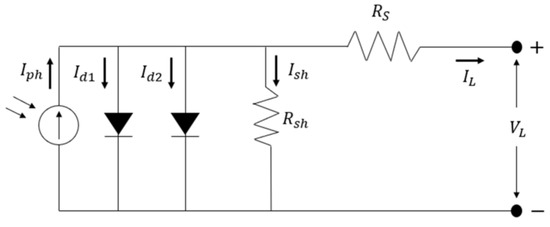
Figure 2. DDM circuit structure in PV systems [36].

Here, $I_{d2}$ stands for saturation current, n₁ and n₂ represent the ideal saturation coefficient of two diodes, and $I_{d1}$ is the diode emission current. DDM needs to extract seven different parameters ($I_{ph}$, $I_{d1}$, $I_{d2}$, $R_S$, $R_{sh}$, $n_1$, and $n_2$).

3.3. PV Module Modeling

Figure 3 shows the PV module’s circuit diagram with numerous PV cells connected in parallel or series. I_L is calculated using Equation (6):

$$I_L=N_P\cdot I_{ph}-N_P\cdot I_d\cdot \left[\exp \left(\frac{q\cdot \left(V_L/N_S+R_S\cdot I_L/N_P\right)}{n\cdot k\cdot T}\right)-1\right]-\frac{N_P\cdot V_L/N_S+R_S\cdot I_L}{R_{sh}}$$

(6)

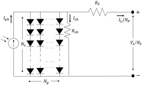
Figure 3. Equivalent circuit of a PV module [36].

The terms N_S and N_P represent the quantity of parallel and serial connections between PV cells. The SDM of PV modules is used in this research. The PV module should determine five unknowns (I_ph, I_d, R_S, R_sh, and n).

3.4. Objective Function

The discrepancy between the determined calculated value and the actual measured value is objectively assessed using an objective function. The calculated data points of the SDM, DDM, and PV modules and error functions for the experiments are represented by Equations (7)–(9).

$$\left\{\begin{array}{c}{f}_{SD}\left(V_L,I_L,\mathit{X}\right)=I_L-I_{ph}+I_{d^{\mathrm{*}}}\left[\exp \left(\frac{q\left(V_L+R_g-I_L\right)}{n-kT}\right)-1\right]+\frac{V_L+R_S\cdot I_L}{R_{\mathrm{L}\mathrm{h}}}\\ \mathit{X}=\left\{I_{\mathrm{p}\mathrm{h}},I_d,R_S,R_{\mathrm{sh} },n\right\}\end{array}\right.$$

(7)

$$\left\{\begin{array}{c}{f}_{DD}\left(V_L,I_L,\mathit{X}\right)=I_L-I_{ph}+I_{d1}\cdot \left[\exp \left(\frac{q\left(V_L+R_S\cdot I_L\right)}{n_1\cdot kT}\right)-1\right]\\ +I_{d2}\cdot \left[\exp \left(\frac{q-\left(V_L+R_s-I_L\right)}{n_2\cdot k-T}\right)-1\right]+\frac{V_L+R_S\cdot I_L}{R_{sh}}\\ \mathit{X}=\left\{I_{ph},I_{dd},I_{d2},R_S,R_{sh},n_1,n_2\right\}\end{array}\right.$$

(8)

$$\left\{\begin{array}{c}{f}_{MD}\left(V_L,I_L,\mathit{X}\right)=I_L-N_P\cdot I_{Mh}+N_P\cdot I_d\cdot \left[\exp \left(\frac{q\left(V_L/N_s+R_S\cdot I_L/N_P\right)}{n\cdot k\cdot T}\right)-1\right]\\ +\frac{N_P\cdot V_L/N_S+R_y\cdot I_L}{R_{sh}}\\ \mathit{X}=\left\{I_{ph},I_d,R_S,R_{sh},n\right\}\end{array}\right.$$

(9)

Equation (10) employs RMSE as an objective function to objectively assess the total disparity between experimental and calculated data.

$$\mathrm{RMSE}(\mathit{X})=\sqrt{\frac{1}{N}{\sum }_{k=1}^N f_k{\left(V_L,I_L,\mathit{X}\right)}^2}$$

(10)

In this formula, X represents the solution consisting of different unknown parameters, and N shows the number of actual measured data.

3.5. Error Metrics

The paper investigates PV parameter extraction using the firefly algorithm, emphasizing its accuracy in estimating parameters for solar cells and PV modules. A three-step methodology assesses the algorithm’s efficacy, comparing its performance with other methods and evaluating error metrics like RE and IAE. The results indicate the firefly algorithm’s superior performance and accuracy, confirming its effectiveness in PV parameter estimation compared to alternative algorithms [37].

In the reference [20], analysis of error metrics such as RMSE reveals TSA’s superior accuracy in parameter extraction compared to other algorithms. TSA exhibits faster convergence and greater stability, as evidenced by fewer outliers in box plots, indicating its efficiency in finding optimal solutions. TSA’s superiority in parameter estimation affirms its effectiveness in addressing PV module problems and accurately determining optimized parameters.

3.6. Coati Optimization Algorithm

The southwest region of Mexico, the United States, South America, and Central America are all home to coatis, which are mammals. Coatis have tiny ears, narrow skulls, black paws, and long, stiff tails. Their noses are flexible, elongated, and slightly upturned. Coatis resemble huge domestic cats in size. They stand about 30 cm tall and range in weight from 2 to 8 kg. Coatis have protruding, pointy teeth. Figure 4 displays a picture of a coati. As omnivores, they consume rodents, lizards, tiny birds, and bird eggs. The green iguana is one of the coati’s favorite foods. The coatis follow these enormous lizards in packs because they are frequently found in trees. Coatis, however, run the risk of being attacked by hunters. Some of the coati’s predators include jaguars, foxes, and wolves.

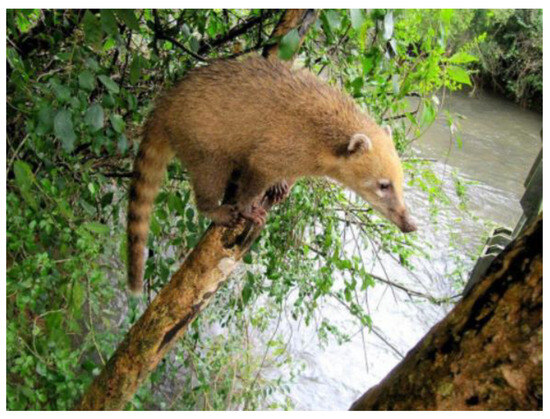
Figure 4. The coati, a mammal [15].

The coatis’ tactics in taking on the iguanas and their actions in fending off and escaping from the predators are highly intelligent. The assault and escape behavior of coatis serves as the basis for the coati optimization algorithm. The coatis are seen as population members of the COA algorithm, a population-based meta-heuristic algorithm. Hence, the coati’s position is a candidate solution for solving the problem in COA. In the first phase of the COA algorithm, several random candidate solutions are created (Equation (11)) [15].

$$\begin{array}{l}{X}_i:x_{i,j}=l{b}_j+r\cdot \left(u{b}_j-l{b}_j\right),i=1,2,\dots ,N,\\ j=1,2,\dots ,m,\end{array}$$

(11)

In this expression, $X_i$ represents a solution for i, where j denotes the desired solution’s dimension. $u{b}_j$ and $l{b}_j$ indicate the upper and lower bounds of dimension j for solution i, with N being the total number of solutions, m representing the number of decision variables, and r representing a random real number ranging from 0 to 1. The initial population of the algorithm (Equation (12)) is stored in a matrix-like X [15].

$$X={\left[\begin{array}{c}{X}_1\\ ⋮\\ X_i\\ ⋮\\ X_N\end{array}\right]}_{N\times m}={\left[\begin{array}{ccccc}{x}_{\mathrm{1,1}}& \cdots & x_{1,j}& \cdots & x_{1,m}\\ ⋮& \ddots & ⋮& \ddots & ⋮\\ x_{i,1}& \cdots & x_{i,j}& \cdots & x_{i,m}\\ ⋮& \ddots & ⋮& \ddots & ⋮\\ x_{N,1}& \cdots & x_{N,j}& \cdots & x_{N,m}\end{array}\right]}_{N\times m}$$

(12)

Each population is evaluated under the influence of the objective function. Each solution is evaluated using Equation (13). The objective function’s value for the $X_i$ solution is represented by ${F(X}_i)$ [15]. Also, here, $F$ represents the vector of the obtained objective function, and $F_i$ signifies the objective function value obtained based on the $h_i$th coati.

$$F={\left[\begin{array}{c}{F}_1\\ ⋮\\ F_i\\ ⋮\\ F_N\end{array}\right]}_{N\times 1}={\left[\begin{array}{c}F\left(X_1\right)\\ ⋮\\ F\left(X_i\right)\\ ⋮\\ F\left(X_N\right)\end{array}\right]}_{N\times 1}$$

(13)

The process of updating the solutions in the COA algorithm depends on modeling the following natural behaviors:

▪

The strategy of coatis when they attack iguanas;

▪

The coatis’ escape strategy to save themselves from hunters.

Based on these two phases, the COA population is updated.

In the first phase, the iguana is hunted and attacked (the exploration phase). Based on a simulation of their attack method on iguanas, the initial stage is modeled when the coati population is updated in the search space. This tactic involves a coati group scaling a tree to come closer to an iguana and startle it. Next, a few coatis wait until the iguana hits the ground under a tree. The coatis attack and hunt the iguana after it hits the ground. This tactic forces coatis to move around in the search area, showcasing COA discovery’s prowess in the global search for problem solving. Figure 5 illustrates the exploratory search method using this approach [15].

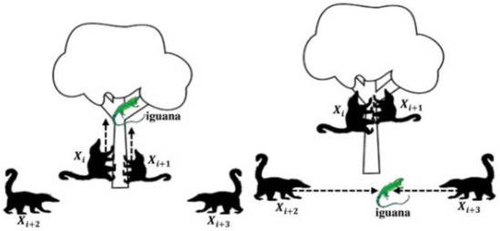
Figure 5. Coatis scaring the prey, the iguana falling on the ground, and coatis hunting it [15].

The iguanas’ position in the COA algorithm corresponds to the population’s top performer position. Furthermore, it is believed that half of the coati group ascends the tree, while the remaining half waits for the iguana to fall. Equation (14) demonstrates the positioning of the coatis as they climb the tree. [15].

$$X_i^{P1}:x_{i,j}^{P1}=x_{i,j}+r\cdot \left({\mathrm{I}\mathrm{g}\mathrm{u}\mathrm{a}\mathrm{n}\mathrm{a}}_j-I·x_{i,j}\right), i=1,2,\dots ,⌊\frac{N}{2}⌋ \mathrm{and} j=1,2,\dots ,m$$

(14)

The iguana that falls on the ground is placed randomly in a search space. The coatis on the ground move within the search space, and this process is simulated using Equations (15) and (16) [15].

$${\mathrm{I}\mathrm{g}\mathrm{u}\mathrm{a}\mathrm{n}\mathrm{a}}^G:{\mathrm{I}\mathrm{g}\mathrm{u}\mathrm{a}\mathrm{n}\mathrm{a}}_j^G=l{b}_j+r\cdot \left(u{b}_j-l{b}_j\right),j=1,2,\dots ,m$$

(15)

$$\begin{array}{c}{X}_i^{P1}:x_{i,j}^{P_1}=\left\{\begin{array}{r}{x}_{i,j}+r\cdot \left({\mathrm{I}\mathrm{g}\mathrm{u}\mathrm{a}\mathrm{n}\mathrm{a}}_j^G-I\cdot x_{i,j}\right),F_{{\mathrm{I}\mathrm{g}\mathrm{u}\mathrm{a}\mathrm{n}\mathrm{a}}^G}<F_i\\ x_{i,j}+r\cdot \left(x_{i,j}-{\mathrm{I}\mathrm{g}\mathrm{u}\mathrm{a}\mathrm{n}\mathrm{a}}_j^G\right),\mathrm{e}\mathrm{l}\mathrm{s}\mathrm{e}\end{array}\right.\\ \mathrm{f}\mathrm{o}\mathrm{r} i=⌊\frac{N}{2}⌋+1,⌊\frac{N}{2}⌋+2,\dots ,N \mathrm{a}\mathrm{n}\mathrm{d} j=1,2,\dots ,m\end{array}$$

(16)

Each solution is updated if the objective function’s value is more optimal for the new position, and Equation (17) is used [15].

$$X_i=\left\{\begin{array}{rr}{X}_i^{P_1},& F_i^{P_1}<F_i,\\ X_i,& \hfill \mathrm{e}\mathrm{l}\mathrm{s}\mathrm{e}\hfill \end{array}\right.$$

(17)

In this equation, $X_i^{P_1}$ is a new position, and the value of the objective function for it is equal to $F_i^{P_1}$; r is a random number between zero and one; I is a random number (either 1 or 2). The objective function’s value for the position of the iguana is represented by $F_{{\mathrm{I}\mathrm{g}\mathrm{u}\mathrm{a}\mathrm{n}\mathrm{a}}^G}$ and ${\mathrm{I}\mathrm{g}\mathrm{u}\mathrm{a}\mathrm{n}\mathrm{a}}_j^G$; the next position, j, is an iguana on the ground. The procedure of fleeing from predators (the exploitation phase) is carried out in the second phase. A coati retreats from its place when a predator attacks it.

In this case, the coati escapes to the current position’s surroundings; an example of this behavior is shown in Figure 6. The coati’s escape behavior is formulated in Equations (18) and (19). According to Equation (20), the relocation is complete if the new position is more optimal than the current one [15].

$$l{b}_j^{\mathrm{l}\mathrm{o}\mathrm{c}\mathrm{a}\mathrm{l}}=\frac{l{b}_j}{t},u{b}_j^{\mathrm{l}\mathrm{o}\mathrm{c}\mathrm{a}\mathrm{l}}=\frac{u{b}_j}{t},$$

(18)

where $t=1,2,\dots ,T$ and $i=1,\dots ,N,j=1,\dots ,m$.

$$X_i^{P2}:x_{i,j}^{P2}=x_{i,j}+(1-2r)\cdot \left(l{b}_j^{\mathrm{l}\mathrm{o}\mathrm{c}\mathrm{a}\mathrm{l}}+r\cdot \left(u{b}_j^{\mathrm{l}\mathrm{o}\mathrm{c}\mathrm{a}\mathrm{l}}-l{b}_j^{\mathrm{l}\mathrm{o}\mathrm{c}\mathrm{a}\mathrm{l}}\right)\right)$$

(19)

$$X_i=\left\{\begin{array}{rr}{X}_i^{P2},& F_i^{P2}<F_i\\ X_i,& \hfill \mathrm{e}\mathrm{l}\mathrm{s}\mathrm{e}\hfill \end{array}\right.$$

(20)

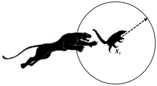
Figure 6. Coati’s escape from the current position [15].

Here, $u{b}_j^{\mathrm{l}\mathrm{o}\mathrm{c}\mathrm{a}\mathrm{l}}$ and $l{b}_j^{\mathrm{l}\mathrm{o}\mathrm{c}\mathrm{a}\mathrm{l}}$ are each dimension’s upper and lower limits, t is the repetition counter of the algorithm, $X_i^{P2}$ is the new position of a coati based on the escape process, T is the maximum number of repetitions of the COA algorithm, and r is a random number between zero and one. A suitable approach to increase the accuracy of the COA algorithm is to use chaotic functions such as tent. The chaos function’s role is to enhance the COA algorithm’s global search. In the local optimum, the chaos function such as tent executes the random variables in the COA algorithm with a more random behavior and reduces the probability of getting caught. In Equation (21), the tent chaos function is formulated [12].

$$z_{k+1}=\left\{\begin{array}{cc}{z}_k/\beta ,& 0<z_k\le \beta \\ \left(1-z_k\right)/(1-\beta ),& \beta <z_k\le 1\end{array}\right.$$

(21)

In this equation, $z_0=0.125$ and $\beta =2.59$. In Figure 7, the tent chaos function is shown.

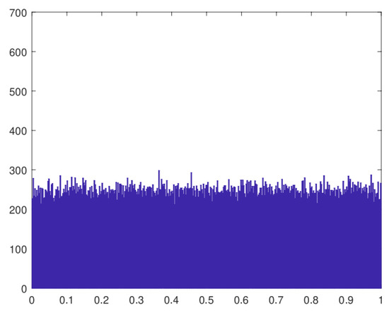
Figure 7. Chaos function to create more chaos in the COA algorithm [12].

Figure 7 demonstrates the application of the tent chaos function within the COA algorithm to introduce heightened chaos, aiding in the comprehensive exploration of the search space. Moreover, the COA algorithm integrates opposition-based learning to effectively initialize the population, leading to accelerated convergence rates. This approach ensures a more exhaustive search of the problem space and facilitates the attainment of optimal solutions, thereby enhancing the efficiency of the algorithm’s convergence.

Initialization: A new population develops in the solution space at the opposite end of the current position using the opposition-based learning technique. The benefit is that there is a 50% chance that the two opposites are closer to the ideal answer. Equations (22) and (23) give the mathematical expressions for the current and the reverse populations, respectively:

$$X_{i,j}=L{b}_j+z_{i,j}\left(U{b}_j-L{b}_j\right)$$

(22)

$$O{X}_{i,j}=b_j+L{b}_j-X_{i,j}$$

(23)

$U{b}_j$ and $L{b}_j$ represent the lower and upper limits of dimension j, $O{X}_{i,j}$ is the reciprocal position, and $X_{i,j}$ is the current solution to the problem. Here, $b_j$ is the center between the solution $X_{i,j}$ and its reciprocal solution or $O{X}_{i,j}$, which is calculated using Equation (24):

$$b_j=\left|X_{i,j}-\frac{U{b}_j+L{b}_j}{2}\right|$$

(24)

3.7. Proposed Flowchart

In the proposed flowchart depicted in Figure 8, the steps for optimizing the parameters of solar cells using the COA algorithm are outlined. These steps include setting up the algorithm parameters, generating an initial population of solutions, evaluating the objective function, updating solutions through various mechanisms, and implementing opposition-based learning. The flowchart serves as a guide for determining the characteristics of solar cells and optimizing their parameters.

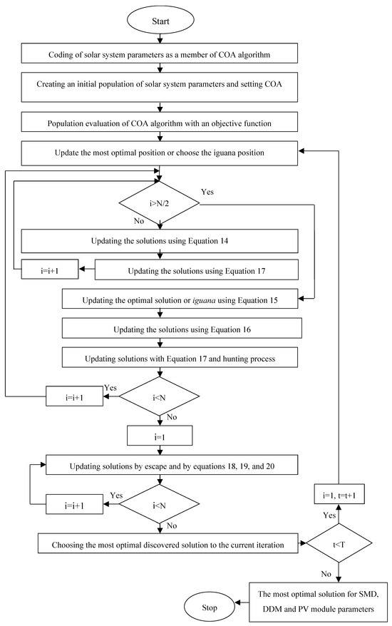
Figure 8. Flowchart of the proposed method.

Each solution is a set of PV circuit parameters in the proposed method. If the type of circuit is SMD, each solution is (I_ph, I_d, R_S, R_sh, and n). If the circuit type is DDM, each solution is (I_ph, I_d1, I_d2, R_S, R_sh, n₁, and n₂). Finally, if the circuit type is a PV module, five variables (I_ph, I_d, R_S, R_sh, and n) offer a solution to the COA algorithm. Figure 8 depicts the suggested technique’s flowchart for determining solar cell characteristics. The following are the steps of the suggested strategy for optimizing the circuit parameters of solar cells:

▪

Start;

▪

The parameters of SMD, DDM, and PV modules are coded as members of the COA algorithm;

▪

Set parameters of the COA algorithm;

▪

Set the algorithm counter to t = 1;

▪

Create an initial population of random COA algorithm solution;.

▪

Evaluate objective function to find solutions;

▪

Determine the most optimal solution, i.e., iguanas, in each iteration;

▪

Increase the COA algorithm repetition counter by one unit;

▪

Find chaos parameters of the COA algorithm;

▪

Update half of the solutions (coatis that have climbed trees);

▪

Update half of the solutions (coatis) with the hunting mechanism of the iguana falling on the ground;

▪

Update solutions using predator escape mechanism;

▪

Implement opposition-based learning;

▪

In each iteration, evaluate the population and solutions and choose the most optimal solution;

▪

Repeat steps of the COA algorithm;

▪

Select the most optimal solution or parameters of SMD, DDM, and PV modules in the last iteration;

▪

Optimize the parameters of the solar module circuit;

▪

Stop.

This article addresses the urgent need to improve the efficiency of PV systems by fine-tuning their parameters. This need is driven by the escalating worldwide demand for electricity and mounting concerns regarding environmental degradation and the limited availability of fossil fuels. By introducing an innovative method that integrates the COA with chaotic functions, the paper endeavors to overcome the obstacles associated with precisely optimizing parameters within PV modules and solar cells.

The fundamental necessities outlined in this article are presented in Table 3.

Table 3. The advantages of solar PV systems.

Requirements	Description
Optimization of solar PV parameters	Maximize the efficiency of solar PV systems by accurately optimizing their parameters.
Reduction in environmental impact	Mitigate environmental pollution and reduce reliance on non-renewable energy sources like fossil fuels.
Advancement of optimization techniques	Represents a significant advancement in optimization techniques for solar PV systems.
Enhanced stability and accuracy	Improve the stability and accuracy of parameter optimization in PV modules and solar cells, thereby increasing the reliability and performance of solar energy systems.

3.8. The Challenges Tackled by This Paper

The challenges tacked by this paper comprise the following:

• Complexity of Parameter Optimization: The process of optimizing parameters within PV modules and solar cells entails grappling with intricate mathematical models and inherent uncertainties stemming from fluctuations in solar radiation and temperature;
• Requirement for Improved Optimization Algorithms: Traditional optimization algorithms may encounter difficulties in adequately managing the intricacies of parameter optimization within solar PV systems, underscoring the necessity for novel approaches such as the COA algorithm proposed herein;
• Attaining Global Optima: The task of identifying the global optimum solution for parameter optimization in solar PV systems is arduous due to the existence of numerous local optima and the expansive search space with high dimensions.

3.9. The Contributions Made by This Paper to the Field

The contributions made by this paper to the corresponding field are as follows:

(1)

Innovative Optimization Strategy: Introducing a fresh optimization strategy utilizing the COA algorithm and chaotic functions, which exhibits superior effectiveness compared to existing meta-heuristic algorithms in terms of minimizing RMSE and standard deviation;

(2)

Enhanced Parameter Optimization: The proposed approach ensures more precise and consistent optimization of parameters within SDM, DDM, and PV modules, consequently improving power generation efficiency and the overall reliability of solar PV systems;

(3)

Potential for Future Research: The paper outlines future research prospects, including the exploration of LSTM neural networks for optimizing solar cell parameters and forecasting solar radiation and panel temperature. This indicates promising avenues for advancing techniques in solar energy optimization.

4. Results and Discussion

The suggested approach is based on four popular PV models that were applied and proven through SDM assault in the DDM attack in the RTC France cell, RTC France cell, STP6-120/36 module, and Photowatt-PWP201 module. Current-voltage data for DDM and SDM were measured on a 57 mm diameter commercial silicon RTC. At 33 °C, French solar cells were measured below 1000 W/m². A total of 36 polycrystalline silicon cells comprising a Photowatt-PWP201 module were linked in series, and at 45 °C, the current-voltage data were measured. Moreover, a total of 36 polycrystalline silicon cells, measured at 55 °C, made up the STP6-120/36 modules. A few earlier investigations were studied to gather the STP6-120/36 module’s current-voltage measurement data [29,38]. The proposed algorithm was implemented on the MATLAB 2021 platform using an Intel^® i7-HQ CPU with 16 GB memory. Through parameter optimization for distinct PV modules employing the COA, the approach not only boosts output power but also reduces errors and standard deviation, surpassing traditional algorithms such as ITLBO, JSO, CPMPSO, WOA, SCA, GNDO, and MJSO. Furthermore, it outperformed competing algorithms in terms of RMSE and standard deviation, indicating its superior performance and suitability across various circuit configurations. Additionally, the method’s efficient execution time further bolsters its practical applicability. In summary, these results underscore the effectiveness and versatility of the proposed method in tackling diverse optimization challenges within solar energy systems.

4.1. The Range of Parameters

Table 4 demonstrates the SM55 and ST40 parameters, specifically their upper and lower ranges. In addition to the parameters used to implement the proposed algorithm, the number of repetitions is the considered variable, and the population size is 50. In the COA algorithm, r has a random value between zero and one, and I equals a random number that equals 1 or 2. The values of the chaotic function in the proposed method were set at z_0 = 0.125 and β = 2.59.

Table 4. Lower and upper range in the modules [31].

Parameters	Low Range	Upper Range
$I_{ph}\left(A\right)$	0	2∗$I_{sc}$
$I_{sd}\left(A\right)$	0	100 × 10−6
$R_s\left(\Omega \right)$	0	2
$R_{sh}\left(\Omega \right)$	0	5000
n, $n_1$,$n_2$	1	4

4.2. Results Based on SDM

Table 5 displays the optimal parameters’ values extracted for the SDM circuit in the proposed method, namely the improved COA (ICOA), and compares ITLBO, JSO, CPMPSO, WOA, SCA, GNDO, MJSO, and COA. The experiments showed that all meta-heuristic algorithms except WOA and SCA have minimized RMSE values.

Table 5. Comparison among optimal values of parameters in SDM.

Algorithms	${\mathit{I}}_{\mathit{p}\mathit{h}}\left(\mathit{A}\right)$	${\mathit{I}}_{\mathit{s}\mathit{d}}\left(\mathit{A}\right)$	${\mathit{R}}_{\mathit{s}}(\mathsf{\Omega })$	${\mathit{R}}_{\mathit{s}\mathit{h}}(\mathsf{\Omega })$	n	RMSE
ITLBO [21]	0.76078	3.11 × 10−7	0.03654	52.8897	1.47726	0.000773006
JSO [22]	0.76079	3.11 × 10−7	0.03654	52.8882	1.47727	0.000773006
CPMPSO [39]	0.76078	3.11 × 10−7	0.03654	52.8897	1.47726	0.000773006
WOA [38]	0.76162	3.86 × 10−7	0.03530	45.9308	1.49953	0.001085820
SCA [29]	0.7582	4.09 × 10−7	0.03595	68.8388	1.50500	0.002483415
GNDO [30]	0.76078	3.11 × 10−7	0.03654	52.8897	1.47726	0.000773006
MJSO [31]	0.76078	3.11 × 10−7	0.03654	52.8897	1.47726	0.000773006
COA [15]	0.76078	3.11 × 10−7	0.03654	52.8897	1.47726	0.000773006
ICOA (proposed method)	0.76078	3.11 × 10−7	0.03654	52.8897	1.47726	0.000773006

Figure 9 displays the I-V and P-V characteristic curves based on the ICOA’s extracted optimal parameters for SDM. It is clear from Figure 9 that there is a good agreement between the measured and simulated ICOA data.

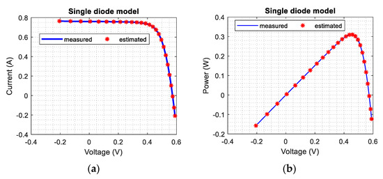
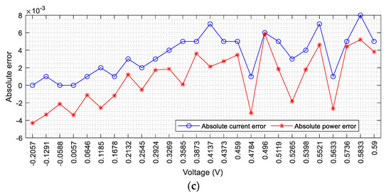
Figure 9. Comparison of the measured and estimated data obtained by ICOA for SDM: (a) I-V characteristic, (b) P-V characteristic, and (c) IAE curves.

4.3. Results Based on DDM

Table 6 compares the value of optimal parameters extracted for the DDM circuit using the proposed method, ITLBO, JSO, CPMPSO, WOA, SCA, GNDO, MJSO, and COA.

Table 6. Comparison among optimal values of parameters of DDM.

Algorithms	${\mathit{I}}_{\mathit{p}\mathit{h}}\left(\mathit{A}\right)$	${\mathit{I}}_{\mathit{s}\mathit{d}1}\left(\mathit{A}\right)$	Rs(Ω)	Rsh(Ω)	n1	${\mathit{I}}_{\mathit{s}\mathit{d}2}\left(\mathit{A}\right)$	n2	RMSE
ITLBO [21]	0.7608	2.47 × 10−7	0.0368	53.9599	1.4579	4.78 × 10−7	1.9949	0.000742264
JSO [22]	0.7608	5.38 × 10−7	0.0371	54.4640	1.7980	1.61 × 10−7	1.4262	0.000754167
CPMPSO [39]	0.7608	7.03 × 10−8	0.0378	56.2715	1.3642	1.00 × 10−6	1.7963	0.000741937
WOA [38]	0.7608	2.67 × 10−7	0.0368	51.8538	1.4662	4.10 × 10−8	1.6133	0.000776464
SCA [29]	0.7684	0.00 × 10+0	0.0324	38.3064	1.1740	3.84 × 10−7	1.4970	0.007351184
GNDO [30]	0.7608	1.00 × 10−6	0.0373	55.6033	1.9051	1.40 × 10−7	1.4130	0.000742327
MJSO [31]	0.7608	7.03 × 10−8	0.0378	56.2715	1.3642	1.00 × 10−6	1.7963	0.000741937
COA [15]	0.7607	7.01 × 10−8	0.0377	56.2716	1.3641	1.00 × 10−6	1.7964	0.000741936
ICOA (proposed method)	0.7608	7.02 × 10−8	0.0377	56.2714	1.3642	1.00 × 10−6	1.7962	0.000741936

The comparison and tests results show that in the DDM circuit, the proposed method provided more optimal values for the DDM circuit than the JSO, CPMPSO, WOA, SCA, GNDO, MJSO, and COA methods. The RMSE error index in the proposed method shows a lower value. The COA algorithm ranks second after the proposed method, and the CPMPSO and MJSO algorithms rank third.

Figure 10 displays the I-V and P-V characteristic curves based on the ICOA’s extracted optimal parameters for DDM. It is clear from Figure 10 that there is a good agreement between the measured and simulated ICOA data.

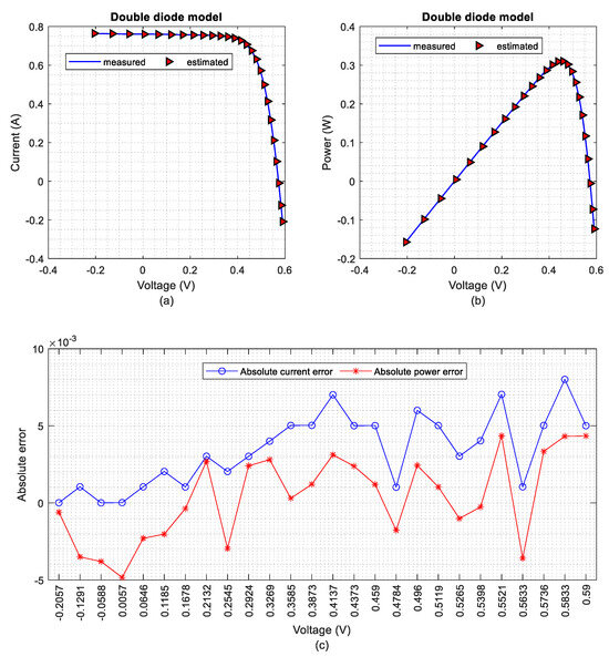
Figure 10. Comparison of the measured and estimated data obtained by ICOA for DDM model: (a) I-V characteristic, (b) P-V characteristic, and (c) IAE curves.

4.4. Results Based on STP6-120/36

Table 7 compares the value of optimal parameters of the STP6-120/36 circuit in the proposed method with similar meta-heuristic methods. The conducted tests show that in the STP6-120/36 circuit, the proposed method’s RMSE value was lower than the meta-heuristic algorithms JSO, CPMPSO, WOA, SCA, GNDO, MJSO, and COA. In these experiments, the COA method’s error is the second lowest in terms of minimum. On the other hand, the experiments show that the CPMPSO, ITLBO, MJSO, and GNDO methods rank third for RMSE error.

Table 7. Comparison among optimal parameter values in STP6-120/36.

Algorithms	${\mathit{I}}_{\mathit{p}\mathit{h}}\left(\mathit{A}\right)$	${\mathit{I}}_{\mathit{s}\mathit{d}}\left(\mathit{A}\right)$	${\mathit{R}}_{\mathit{s}}(\mathsf{\Omega })$	${\mathit{R}}_{\mathit{s}\mathit{h}}(\mathsf{\Omega })$	N	RMSE
ITLBO [21]	7.47528	1.93 × 10−6	0.16891	570.1972	44.80042	0.014251063
JSO [22]	7.47525	1.93 × 10−6	0.16890	571.5660	44.80254	0.014251066
CPMPSO [39]	7.47528	1.93 × 10−6	0.16891	570.1975	44.80042	0.014251063
WOA [38]	7.50318	3.27 × 10−6	0.15781	307.7831	46.40846	0.017581962
SCA [29]	7.56027	1.70 × 10−6	0.17318	323.9495	44.38346	0.052443825
GNDO [30]	7.47528	1.93 × 10−6	0.16891	570.1972	44.80042	0.014251063
MJSO [31]	7.47528	1.93 × 10−6	0.16891	570.1975	44.80042	0.014251063
COA [15]	7.47528	1.92 × 10−6	0.16891	570.1975	44.80041	0.014251063
ICOA (proposed method)	7.47528	1.93 × 10−6	0.16891	570.1974	44.80041	0.014251063

According to the experimentation, the worst algorithm for this situation is the SCA algorithm, which has the highest error among the compared algorithms.

Figure 11 displays the I-V and P-V characteristic curves based on the ICOA’s extracted optimal parameters for STP6-120/36. It is clear from Figure 11 that there is a good agreement between the measured and simulated ICOA data.

Figure 11. Comparison of the measured and estimated data obtained by ICOA for STP6-120/36 model, (a) I-V characteristic, (b) P-V characteristic, and (c) IAE curves.

4.5. Ranking

This section discusses the ranking of the proposed algorithm and competing algorithms such as WOA, GWO, HHO, AVOA, and COA in two error indicators, namely RMSE and standard deviation, for SMD, DDM, and PV modules, respectively, which are shown in Figure 12 and Figure 13.

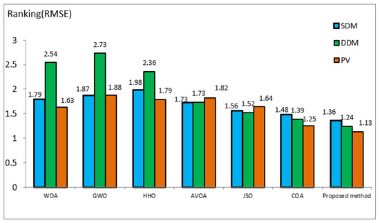
Figure 12. Ranking of algorithms in terms of the minimum RMSE error.

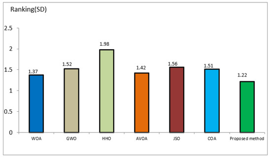
Figure 13. Algorithm ranking based on standard deviation (SD) index.

In the experiments, Friedman’s test was applied to rank different algorithms. In Friedman’s test, any algorithm that shows a lower value has a better ranking to find the optimal solution. A lower number means the algorithm has obtained a better ranking in finding the optimal solution.

According to the experiments, if the circuit is SDM-type, the ranking of WOA, GWO, HHO, AVOA, JSO, COA algorithm, and the proposed method is 1.79, 1.87, 1.98, 1.73, 1.56, 1.48, and 1.36, respectively. In this case, the proposed method obtained the best ranking, and HHO showed the worst performance.

Experiments pertaining to the DDM circuit show that the ranks of algorithms, including WOA, GWO, HHO, AVOA, JSO, COA, and the proposed method for calculating the minimum RMSE are 2.54, 2.73, 2.36, 1.73, 1.52, 1.39, and 1.24, respectively, and the proposed method ranks best in minimizing RMSE. The PV circuit’s rating values of WOA, GWO, HHO, AVOA, JSO, COA, and the proposed method are 1.63, 1.88, 1.79, 1.82, 1.64, 1.25, and 1.13, respectively, so the proposed method again showed the top performance.

Based on the simulations conducted in MATLAB, the proposed method ranks first in the optimization of SDM, DDM, and PV parameters. The proposed method also increases the optimal calculation rank in these three circuits by 8.1%, 10.79%, and 9.6%, respectively, compared to the COA algorithm. Figure 13 displays the average rank of meta-heuristic algorithms and the proposed algorithm in the standard deviation index.

Figure 13 compares the standard deviation (SD) of three modes, namely SDM, DDM, and PV, to the SD values of the proposed method and meta-heuristic algorithms. The standard deviation index is an essential and critical index for measuring the optimization stability for optimizing the parameters of DDM, PV, and SDM circuits. The rank of the proposed algorithm in the standard deviation index is equal to 1.22, and it has the lowest standard deviation among the competing algorithms.

This means that the proposed algorithm has more stability in terms of optimizing the parameters of SDM, DDM, and PV circuits than the WOA, GWO, HHO, AVOA, JSO, and COA algorithms. The worst algorithm in terms of stability in finding optimal solutions is the HHO algorithm. The second meta-heuristic algorithm in terms of stability is the WOA algorithm.

4.6. Time Complexity

To ensure equitable comparison, we incorporated outcomes from alternative methods rather than solely relying on external references. Ensuring uniformity, we maintained identical objective functions and parameters across all experiments as outlined in the original papers. Furthermore, each method received an equal number of attempts to address the problem, enabling a fair comparison within comparable computational constraints. By concentrating on methods addressing identical optimization challenges, we assessed the effectiveness of our proposed model against existing approaches within a controlled framework. This method facilitated an impartial and straightforward evaluation of the strengths and limitations of each approach.

The improved COA algorithm has more equations and complexity than the COA algorithm, so it was expected to be more time-consuming than the COA algorithm. However, contrary to the expectation of the ICOA algorithm, it needs fewer iterations to reach an error level because it has faster convergence than the COA algorithm. Figure 14 compares the optimization time of the solar system parameters in the proposed method and other meta-heuristic methods.

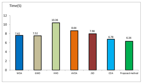
Figure 14. Comparison of the calculation time of optimal PV parameters.

The experiments conducted in MATLAB show that the proposed algorithm’s execution time is about 6.34 s, and it needs less time to reach a certain error level than other algorithms. The performance of the COA algorithm is slightly worse than the proposed method in terms of time index, but it is in second place for execution time. Among the compared algorithms, the worst algorithm in terms of time index is the HHO algorithm. The reason behind the significant execution time of the HHO algorithm is the large number of equations and the high complexity of this algorithm.

5. Conclusions

Global power demand is escalating due to industrial expansion and population growth, with electricity being the primary energy source for industries. However, conventional electricity production methods such as fossil fuels pose environmental challenges. Transitioning to solar energy through PV modules offers a renewable solution to mitigate environmental pollution. Solar cells efficiently convert solar energy into electrical energy, yet their output fluctuates due to varying radiation intensity and angles, posing a challenge for maximizing power generation. To address this, the proposed method utilized the COA to optimize parameters for different PV modules, enhancing output power by minimizing errors and reducing standard deviation compared to conventional algorithms. However, challenges persist, including uncertainty in finding optimal solutions and reliance on precise input data, which may hinder optimization efficacy. Acknowledging practical obstacles like hardware limitations and maintenance complexities is crucial for real-world implementation, underscoring the need for further validation of scalability and applicability in large-scale solar energy systems. Future research could focus on mitigating uncertainty, enhancing algorithm robustness, and integrating predictive modeling techniques like LSTM neural networks to improve parameter optimization and solar energy forecasting, aiming to address the inherent limitations and guide future advancements in solar energy optimization.

References

- Rauf, A.; Nureen, N.; Irfan, M.; Ali, M. The current developments and future prospects of solar photovoltaic industry in an emerging economy of India. Environ. Sci. Pollut. Res. 2023, 30, 46270–46281. [Google Scholar] [CrossRef] [PubMed]
- Yusupov, Z.; Almagrahi, N.; Yaghoubi, E.; Yaghoubi, E.; Habbal, A.; Kodirov, D. Modeling and Control of Decentralized Microgrid Based on Renewable Energy and Electric Vehicle Charging Station. In Proceedings of the 12th World Conference “Intelligent System for Industrial Automation” (WCIS-2022), Tashkent, Uzbekistan, 25–26 November 2022; pp. 96–102. [Google Scholar]
- Toufik, T.; Dekkiche, M.; Denai, M. Techno-Economic Comparative Study of Grid-Connected Pv/Reformer/Fc Hybrid Systems with Distinct Solar Tracking Systems. Energy Convers. Manag. X 2023, 18, 100360. [Google Scholar] [CrossRef]
- Sharma, A.; Sharma, A.; Dasgotra, A.; Jately, V.; Ram, M.; Rajput, S.; Averbukh, M.; Azzopardi, B. Opposition-based tunicate swarm algorithm for parameter optimization of solar cells. IEEE Access 2021, 9, 125590–125602. [Google Scholar] [CrossRef]
- Van Gompel, J.; Spina, D.; Develder, C. Cost-effective fault diagnosis of nearby photovoltaic systems using graph neural networks. Energy 2023, 266, 126444. [Google Scholar] [CrossRef]
- Wu, X.; Liao, B.; Su, Y.; Li, S. Multi-objective and multi-algorithm operation optimization of integrated energy system considering ground source energy and solar energy. Int. J. Electr. Power Energy Syst. 2023, 144, 108529. [Google Scholar] [CrossRef]
- Balamurugan, N.; Karuppasamy, P.; Ramasamy, P. Investigation on Different Crystal Grains from the Multi-crystalline Silicon (mc-Si) Wafer. Silicon 2023, 15, 1465–1474. [Google Scholar] [CrossRef]
- Irshad, A.S. Design and comparative analysis of grid-connected BIPV system with monocrystalline silicon and polycrystalline silicon in Kandahar climate. MATEC Web Conf. 2023, 374, 3002. [Google Scholar] [CrossRef]
- Hamed, S.B.; Abid, A.; Ben Hamed, M.; Sbita, L.; Bajaj, M.; Ghoneim, S.S.; Zawbaa, H.M.; Kamel, S. A robust MPPT approach based on first-order sliding mode for triple-junction photovoltaic power system supplying electric vehicle. Energy Rep. 2023, 9, 4275–4297. [Google Scholar] [CrossRef]
- Kumar, C.M.S.; Singh, S.; Gupta, M.K.; Nimdeo, Y.M.; Raushan, R.; Deorankar, A.V.; Kumar, T.A.; Rout, P.K.; Chanotiya, C.S.; Pakhale, V.D.; et al. Solar energy: A promising renewable source for meeting energy demand in Indian agriculture applications. Sustain. Energy Technol. Assess. 2023, 55, 102905. [Google Scholar] [CrossRef]
- Afzal, A.; Buradi, A.; Jilte, R.; Shaik, S.; Kaladgi, A.R.; Arıcı, M.; Lee, C.T.; Nižetić, S. Optimizing the thermal performance of solar energy devices using meta-heuristic algorithms: A critical review. Renew. Sustain. Energy Rev. 2023, 173, 112903. [Google Scholar] [CrossRef]
- Shorabeh, S.N.; Samany, N.N.; Minaei, F.; Firozjaei, H.K.; Homaee, M.; Boloorani, A.D. A decision model based on decision tree and particle swarm optimization algorithms to identify optimal locations for solar power plants construction in Iran. Renew. Energy 2022, 187, 56–67. [Google Scholar] [CrossRef]
- Wu, H.; Deng, F.; Tan, H. Research on parametric design method of solar photovoltaic utilization potential of nearly zero-energy high-rise residential building based on genetic algorithm. J. Clean. Prod. 2022, 368, 133169. [Google Scholar] [CrossRef]
- Bonthagorla, P.K.; Mikkili, S. A Novel Hybrid Slime Mould MPPT Technique for BL-HC Configured Solar PV System Under PSCs. J. Control. Autom. Electr. Syst. 2023, 34, 782–795. [Google Scholar] [CrossRef]
- Dehghani, M.; Montazeri, Z.; Trojovská, E.; Trojovský, P. Coati Optimization Algorithm: A new bio-inspired metaheuristic algorithm for solving optimization problems. Knowl. Based Syst. 2023, 259, 110011. [Google Scholar] [CrossRef]
- Zhang, Y.; Wu, Y.; Li, L.; Liu, Z. A Hybrid Energy Storage System Strategy for Smoothing Photovoltaic Power Fluctuation Based on Improved HHO-VMD. Int. J. Photoenergy 2023, 2023, 9633843. [Google Scholar] [CrossRef]
- Zadehbagheri, M.; Abbasi, A.R. Energy cost optimization in distribution network considering hybrid electric vehicle and photovoltaic using modified whale optimization algorithm. J. Supercomput. 2023, 79, 14427–14456. [Google Scholar] [CrossRef]
- Aguila-Leon, J.; Vargas-Salgado, C.; Chiñas-Palacios, C.; Díaz-Bello, D. Solar photovoltaic Maximum Power Point Tracking controller optimization using Grey Wolf Optimizer: A performance comparison between bio-inspired and traditional algorithms. Expert Syst. Appl. 2023, 211, 118700. [Google Scholar] [CrossRef]
- Abbassi, A.; Ben Mehrez, R.; Bensalem, Y.; Abbassi, R.; Kchaou, M.; Jemli, M.; Abualigah, L.; Altalhi, M. Improved Arithmetic Optimization Algorithm for Parameters Extraction of Photovoltaic Solar Cell Single-Diode Model. Arab. J. Sci. Eng. 2022, 47, 10435–10451. [Google Scholar] [CrossRef]
- Beşkirli, A.; Dağ, İ. Parameter extraction for photovoltaic models with tree seed algorithm. Energy Rep. 2023, 9, 174–185. [Google Scholar] [CrossRef]
- Li, S.; Gong, W.; Yan, X.; Hu, C.; Bai, D.; Wang, L.; Gao, L. Parameter extraction of photovoltaic models using an improved teaching-learning-based optimization. Energy Convers. Manag. 2019, 186, 293–305. [Google Scholar] [CrossRef]
- Chou, J.-S.; Truong, D.-N. A novel metaheuristic optimizer inspired by behavior of jellyfish in ocean. Appl. Math. Comput. 2021, 389, 125535. [Google Scholar] [CrossRef]
- Patra, B.; Nema, P.; Khan, M.Z.; Khan, O. Optimization of solar energy using MPPT techniques and industry 4.0 modelling. Sustain. Oper. Comput. 2023, 4, 22–28. [Google Scholar] [CrossRef]
- Rayaguru, N.K.; Lindsay, N.M.; Crespo, R.G.; Raja, S.P. Hybrid bat–grasshopper and bat–modified multiverse optimization for solar photovoltaics maximum power generation. Comput. Electr. Eng. 2023, 106, 108596. [Google Scholar] [CrossRef]
- Louzazni, M.; Khouya, A.; Amechnoue, K.; Gandelli, A.; Mussetta, M.; Crăciunescu, A. Metaheuristic algorithm for photovoltaic parameters: Comparative study and prediction with a firefly algorithm. Appl. Sci. 2018, 8, 339. [Google Scholar] [CrossRef]
- Ćalasan, M.; Aleem, S.H.A.; Zobaa, A.F. On the root mean square error (RMSE) calculation for parameter estimation of photovoltaic models: A novel exact analytical solution based on Lambert W function. Energy Convers. Manag. 2020, 210, 112716. [Google Scholar] [CrossRef]
- Nunes, H.; Pombo, J.; Bento, P.; Mariano, S.; Calado, M. Collaborative swarm intelligence to estimate PV parameters. Energy Convers. Manag. 2019, 185, 866–890. [Google Scholar] [CrossRef]
- Abbassi, R.; Saidi, S.; Urooj, S.; Alhasnawi, B.N.; Alawad, M.A.; Premkumar, M. An Accurate Metaheuristic Mountain Gazelle Optimizer for Parameter Estimation of Single- and Double-Diode Photovoltaic Cell Models. Mathematics 2023, 11, 4565. [Google Scholar] [CrossRef]
- Mirjalili, S. SCA: A Sine Cosine Algorithm for solving optimization problems. Knowl. Based Syst. 2016, 96, 120–133. [Google Scholar] [CrossRef]
- Zhang, Y.; Jin, Z.; Mirjalili, S. Generalized normal distribution optimization and its applications in parameter extraction of photovoltaic models. Energy Convers. Manag. 2020, 224, 113301. [Google Scholar] [CrossRef]
- Abdel-Basset, M.; Mohamed, R.; Chakrabortty, R.K.; Ryan, M.J.; El-Fergany, A. An Improved Artificial Jellyfish Search Optimizer for Parameter Identification of Photovoltaic Models. Energies 2021, 14, 1867. [Google Scholar] [CrossRef]
- Perles, L.; Martins, T.F.; Barreto, W.T.G.; de Macedo, G.C.; Herrera, H.M.; Mathias, L.A.; Labruna, M.B.; Barros-Battesti, D.M.; Machado, R.Z.; André, M.R. Diversity and Seasonal Dynamics of Ticks on Ring-Tailed Coatis Nasua nasua (Carnivora: Procyonidae) in Two Urban Areas from Midwestern Brazil. Animals 2022, 12, 293. [Google Scholar] [CrossRef] [PubMed]
- Hasanien, H.M.; Alsaleh, I.; Alassaf, A.; Alateeq, A. Enhanced coati optimization algorithm-based optimal power flow including renewable energy uncertainties and electric vehicles. Energy 2023, 283, 129069. [Google Scholar] [CrossRef]
- Sun, X.; Zhu, L.; Liu, D. Quantification of early bruises on blueberries using hyperspectral reflectance imaging coupled with band ratio and improved multi-threshold coati optimization algorithm method. Microchem. J. 2024, 199, 110078. [Google Scholar] [CrossRef]
- Yin, X.; Tian, H.; Zhang, F.; Li, A. Quantitative analysis of millet mixtures based on terahertz time-domain spectroscopy and improved coati optimization algorithm. Spectrosc. Lett. 2024, 57, 31–44. [Google Scholar] [CrossRef]
- Jian, X.; Cao, Y. A Chaotic Second Order Oscillation JAYA Algorithm for Parameter Extraction of Photovoltaic Models. Photonics 2022, 9, 131. [Google Scholar] [CrossRef]
- Louzazni, M.; Khouya, A.; Amechnoue, K.; Mussetta, M.; Crăciunescu, A. Comparison and evaluation of statistical criteria in the solar cell and photovoltaic module parameters’ extraction. Int. J. Ambient. Energy 2020, 41, 1482–1494. [Google Scholar] [CrossRef]
- Elazab, O.S.; Hasanien, H.M.; Elgendy, M.A.; Abdeen, A.M. Whale optimisation algorithm for photovoltaic model identification. J. Eng. 2017, 2017, 1906–1911. [Google Scholar] [CrossRef]
- Liang, J.; Ge, S.; Qu, B.; Yu, K.; Liu, F.; Yang, H.; Wei, P.; Li, Z. Classified perturbation mutation based particle swarm optimization algorithm for parameters extraction of photovoltaic models. Energy Convers. Manag. 2020, 203, 112138. [Google Scholar] [CrossRef]
Disclaimer/Publisher’s Note: The statements, opinions and data contained in all publications are solely those of the individual author(s) and contributor(s) and not of MDPI and/or the editor(s). MDPI and/or the editor(s) disclaim responsibility for any injury to people or property resulting from any ideas, methods, instructions or products referred to in the content. |
© 2024 by the authors. Licensee MDPI, Basel, Switzerland. This article is an open access article distributed under the terms and conditions of the Creative Commons Attribution (CC BY) license (https://creativecommons.org/licenses/by/4.0/).