1. Introduction
A great number of power transformers are used in electric power systems to convert one voltage class to another. For example, about 461,864 substations are equipped with them in Russia [
1]. Three-phase two-winding asymmetrical transformers are most often used for these purposes due to their high performance.
World practice in operating three-phase transformers has shown turn-to-turn faults to be among the most common short circuits in them. According to [
1,
2], they are up to 70–80% of all transformer failures depending on the power and operating conditions.
One of the main ways of decreasing the statistics of failures and extending the service life of transformers is the use of relay protection devices based on current transformers [
3,
4,
5] and nonconventional high-sensitive protection devices based on inductive measuring transducers [
2,
6]. Such devices can be improved, in particular, their sensitivity to turn-to-turn faults can be increased, by means of receiving information about characteristic features of currents in the transformer windings in the form of the spectrum of harmonic components of the currents during transformer operation. This is especially important for choosing the response threshold of relay protection devices, the operation of which is based on the differential principle, which consists of comparing two electrical quantities with different spectra. Both currents in the transformer windings [
3,
4,
5] and their magnetic leakage fluxes [
2,
6] can be used as compared parameters.
The experimental way of acquiring this information is the easiest. For this, necessary measurements are made during the operation of a three-phase power transformer. However, the comprehensive study of a transformer during its operation is not always possible. For example, currents in the secondary windings attain 150 kA in ore furnace transformers; therefore, current transformers are not installed on them, and currents in the load circuit cannot be measured. Hence, a mathematical simulation is more convenient.
Many mathematical models of transformers have been developed by now for different purposes. Most of these models are reviewed in [
7,
8]. Some of them are intended for the description of the current transformer operation [
9]. The model in [
10] is used for simulating transient processes in a single-phase transformer. The authors of work [
11] suggested using the finite different method for simulating transient processes in network transformers, thus increasing computational costs and requiring an external circuit interface. Reference [
12] suggests an equivalent scheme for determining multiwinding transformer-leakage inductances. The mathematical model proposed by [
13] enables the simulation of three-phase saturating transformers. An equivalent scheme for the real-time simulation of nonlinear power transformers was developed in detail in [
14]. However, the models of [
12,
13,
14] require a significant amount of initial data, thus making these models unsuitable for practical purposes, in particular, when these data should be received from working transformers. Moreover, output of certain models cannot be used to implement relay protection. Thus, to estimate capabilities of known mathematical models in terms of their suitability for use in relay protection, for example, for choosing the differential protection response threshold, one should analyze the purpose of a model, the required transformer modeling mode, the ease of acquiring the initial data for modeling, and results of protection device modeling. Considering all of these points, the quite well-known mathematical model of a three-phase transformer suggested by P. Bastard et al. [
8] for analyzing the processes occurring in the transformer is apparently the most suitable.
This model is based on ElectroMagnetic Transient Program (EMTP-RV4.1) software with BCTRAN package. The BCTRAN package describes a transformer based on data received in different tests. For a three-phase two-winding transformer, BCTRAN computes two sixth-order matrices. One of them is the matrix of resistances of the transformer windings, and another is the matrix of the self-inductances of these windings. However, the use of EMTP hampers comprehension of the model and limits access to internal variables (magnetic couplings) for their analysis—the more so since these couplings are complex.
Reference [
15] shows that the operation of a three-phase transformer can be described without EMTP, but with any other computing software, for example, MATLAB v6.5.
According to [
16], the process of energy conversion in three-phase power transformers is most fully described by a quite simple and easily understandable mathematical model with phase coordinates. In this model, the operation of a three-phase two-winding transformer is described by only four differential equations [
17]. These differential equations are compiled by the loop current method [
18,
19] for phase-to-phase voltages. This mathematical model can be implemented not only in a MATLAB environment, but also in Turbo Basic [
20].
However, this mathematical model does not take into account the nonlinearity of parameters of the magnetic core of a transformer. Self-inductances and mutual inductances are calculated in the differential equations of the mathematical model in a simplified form, neglecting transformer core design features. All of these shortcomings reduce the simulation accuracy and do not enable one to sufficiently and accurately determine the response threshold of, e.g., high-sensitive turn-to-turn fault protections based on built-in inductive measuring transducers [
2,
6].
To get rid of these shortcomings, the mathematical model presented in [
17] as a set of differential equations is transformed into a mathematical model described by a set of linear equations. When simulating steady-state load operation modes of a transformer in this model, the duration of a mode under study is divided into time intervals within which the transformer parameters are considered constant. The initial values of inductances and mutual inductances in the mathematical model are determined using the main inductance of a transformer phase and the ratios of magnetic fluxes in the core legs during the no-load operation of the transformer. The current values of these parameters are calculated from the currents in the windings and magnetic fluxes in the legs of the core of this transformer.
2. Mathematical Model of a Transformer
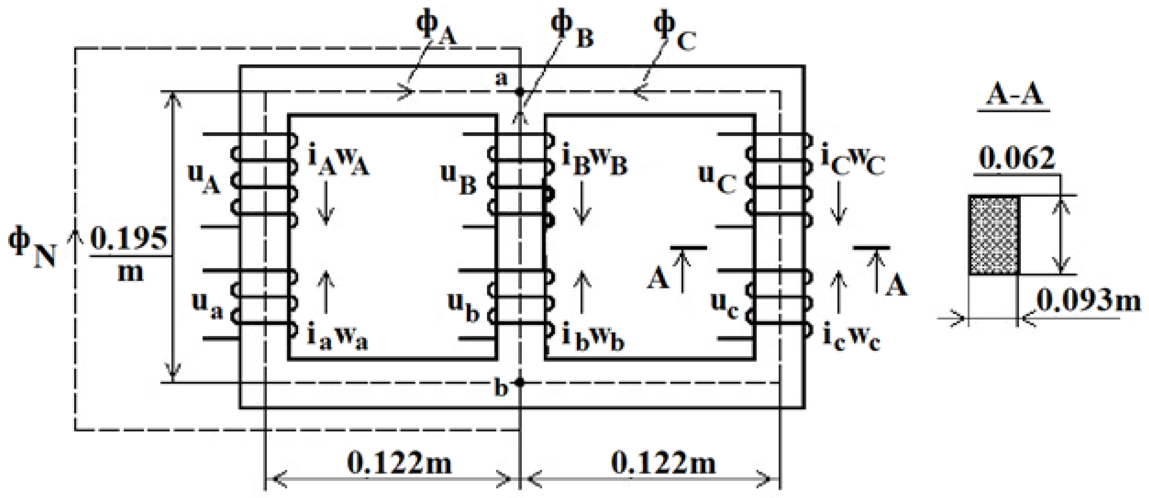
The mathematical model of a transformer [
17], represented as a set of differential equations, is transformed into a mathematical model described by a set of linear equations, taking into account the diagram of the core (
Figure 1) and the electric circuit of the transformer (
Figure 2).
In
Figure 1, u
A, u
B, and u
C (u
a, u
b, and u
c) are the instantaneous values of phase voltages in the primary (secondary) windings of phases A, B, and C (a, b, and c); i
A, i
B, and i
C (i
a, i
b, and i
c) are the instantaneous values of currents in the primary (secondary) windings of phases A, B, and C (a, b, and c); w
A, w
B, and w
C (w
a, w
b, and w
c) are the numbers of turns in the primary (secondary) windings of phases A, B, and C (a, b, and c),
and
; ϕ
A, ϕ
B, and ϕ
c are the magnetic fluxes in the legs of phases A, B, and C of the core; ϕ
N is the magnetic leakage flux.
For the experimental estimation of the simulation error, an experimental 6.0 kVA TT-6-type transformer is used; its parameters are given in
Table 1.
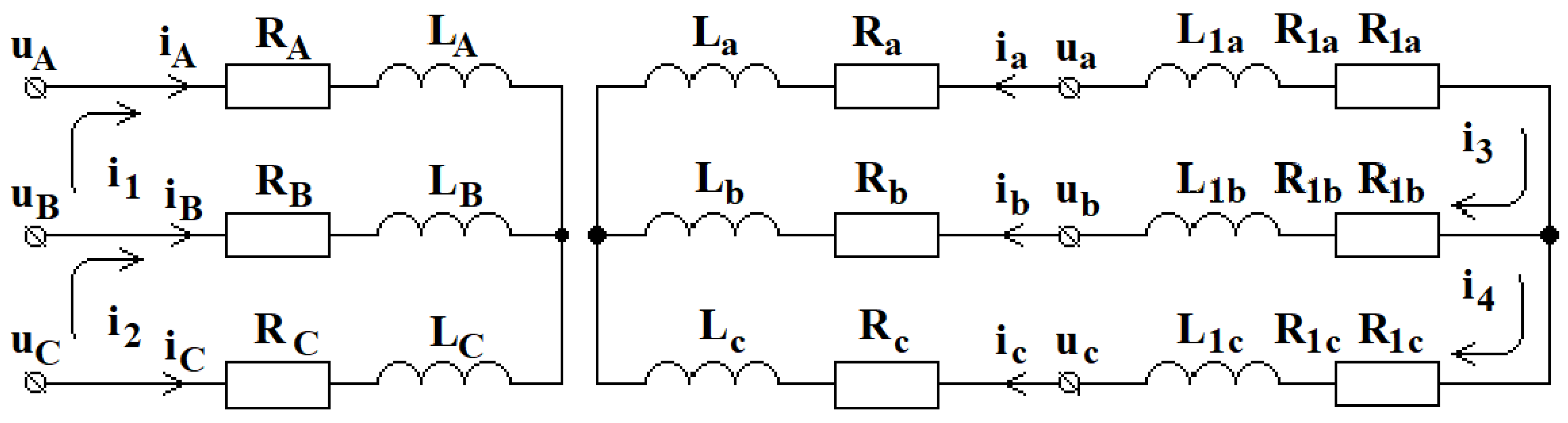
In
Figure 2,
are the instantaneous values of currents in the 1st–4th loops;
, and
are the active resistances of the primary and secondary windings of the transformer equal to R
1 and R
2, respectively; R
la, R
lb, and R
lc are the active resistances of the transformer phase loads.
If the voltages are considered sinusoidal in the mathematical model [
17], then the operator of differentiation,
, in its equations can be changed to the expression
with allowance given [
15]. In this case, the set of equations of this mathematical model is transformed into the set
where
and
are the instantaneous values of the linear voltages of phases A, B, and C; and
are the voltage drops across the inductive resistances and the mutual inductive resistances of the 1st–4th loops:
where X
la, X
lb, and X
lc are the inductive resistances of the transformer load;
; v and w take on values from 1 to 4; and
represents the self-inductances and mutual inductances of the flux linkages of the loops.
The self-inductances in the flux linkages of the loops are defined as
And the mutual inductances are
where
and
are the inductances of the phases of the primary and secondary windings; L
AB and L
BA, L
BC and L
CB, and L
CA and L
AC are the mutual inductances between the phases of the primary winding; and L
ab and L
ba, L
bc and L
cb, and L
ca and L
ac are the mutual inductances between the phases of the secondary winding. Moreover,
;
;
;
;
;
;
;
; and L
Cc and L
cC are the mutual inductances between the phases of the primary and secondary windings.
3. Inductances, Mutual Inductances, and Active Resistances in the Mathematical Model of a Transformer
The calculation of the inductive resistances of the windings of a three-phase transformer in the general form is difficult [
2,
21]. However, if the transformer core is considered non-saturated and the magnetic leakage flux of the windings is neglected, then the main inductive resistance,
, and inductance,
, of a phase can be calculated as follows [
21]:
The accuracy must be acceptable for relay protection. Here, is the impedance of the phase of the primary winding of the transformer, and f is the network frequency. The phase voltage , the no-load current , and the active resistance of the primary winding can be easily found in an experimental way.
If the phase voltage U
2 and load current I
l are known, then the active and inductive resistances of a symmetrical load can be quite accurately found from the following mathematical equations:
where
and
are the active and inductive load resistances; and
and L
l are the load impedance and resistance. The active resistance
can also be easily experimentally determined.
Following [
18], the inductances of the primary and secondary windings of a transformer are determined by the values of the magnetic fluxes ϕ
A, ϕ
B, and ϕ
c in the core legs. The inductance of a winding is proportional to the squared number of turns of the winding.
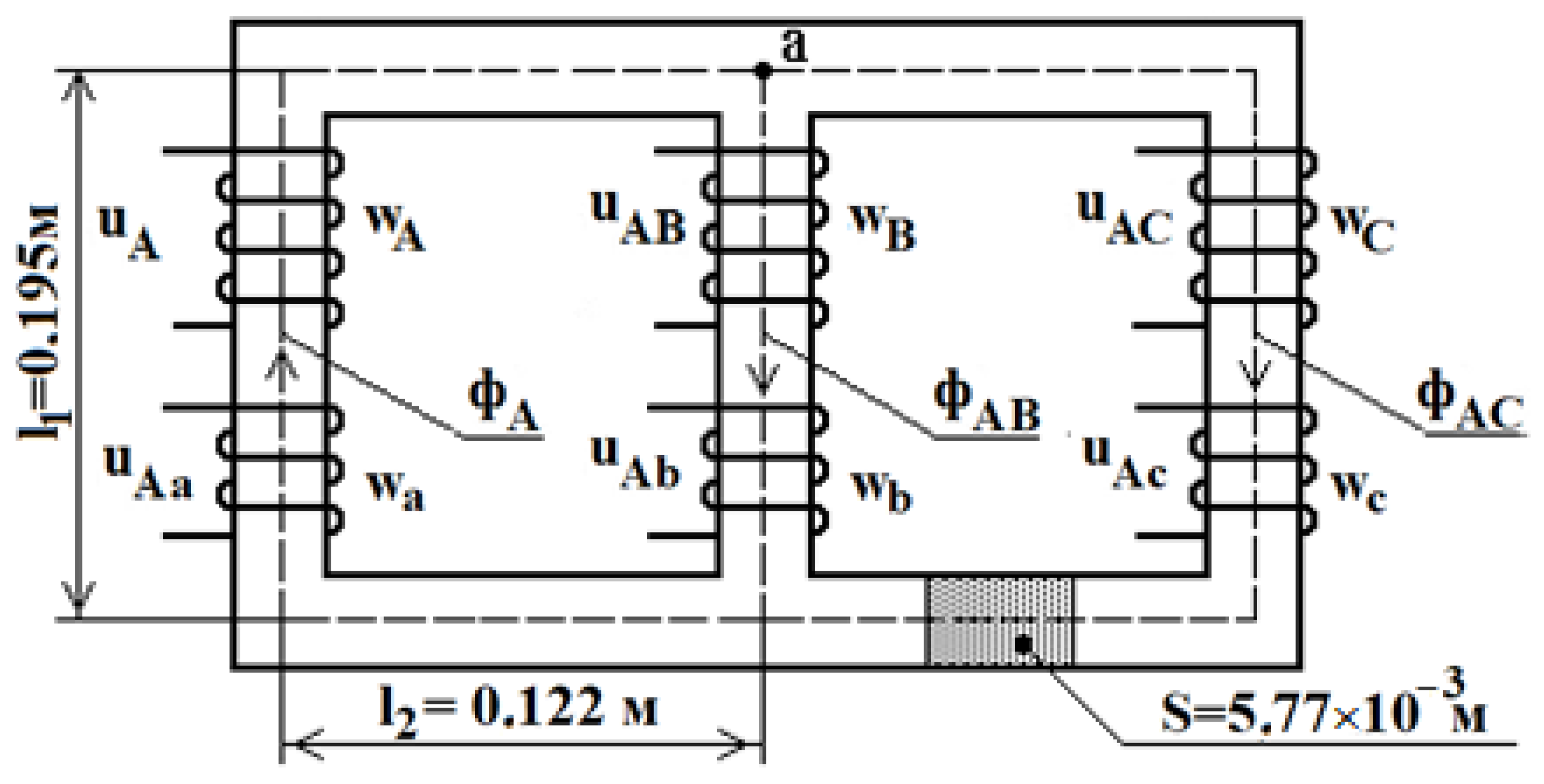
Mutual inductances, for example, between the winding of phase A and other primary windings of the transformer, are determined by the distribution of the magnetic flux of phase A over legs B and C of the transformer.
Figure 3 shows that the magnetic flux of phase A ϕ
A splits into magnetic fluxes ϕ
AB and ϕ
AC at point and then flow through the legs of phases B and C. Just these fluxes determine the magnetic couplings between the winding of phase A and the windings of phases B and C. These magnetic couplings can be represented by the coefficients
The magnitudes of ϕ
AB and ϕ
AC depend on the design features of the core and materials that it is made of. The accurate calculation of these fluxes is a difficult task. However, if we suggest equal cross-sections of the legs and yokes of the transformer core and the permeability of the steel that they are made of, then, taking into account [
18,
19], the ratio of magnetic fluxes, i.e., the coefficients
and
, can be approximately determined as follows.
According to
Figure 3, the lengths of the ϕ
AB and ϕ
AC closing lines in the core are
Since the magnitudes of ϕ
AB and ϕ
AC fluxes are inversely proportional to their path lengths in the core, the coefficients for the experimental TT-6 transformer are
Figure 3 shows that the transformer core is symmetrical about the leg of phase B. Hence, the ϕ
AB and ϕ
AC magnetic fluxes are equal. Therefore, the coefficients are calculated as follows:
The distribution of the magnetic flux of the leg of phase C over the legs of phases B and A is a mirror image of the distribution of the magnetic flux of the leg of phase A over the legs of phases B and C. Therefore, the coefficients KCA and KCB should be taken to be equal to the coefficients KAC and KAB.
We should add that the
,
, and
coefficients should be taken to be equal to unity when calculating the inductances of the primary and secondary windings and closed turns. The inductances of the primary and secondary windings are calculated as follows:
The mutual inductances between the high-voltage winding of phase A and other windings of the transformer can be determined as follows:
The mutual inductances between the high-voltage winding of phase B and other windings of the transformer can be determined as follows:
The mutual inductances between the high-voltage winding of phase C and other windings of the transformer can be determined as follows:
The mutual inductances between the low-voltage winding of phase A and other windings of the transformer can be determined as follows:
The mutual inductances between the low-voltage winding of phase B and other windings of the transformer can be determined as follows:
The mutual inductances between the low-voltage winding of phase C and other windings of the transformer can be determined as follows:
The inductances and mutual inductances of the loops in this mathematical model do not depend on the saturation of the core. Therefore, the model enables the simulation of currents in the windings of only a linear three-phase power transformer under arbitrary symmetrical and asymmetrical steady-state operation modes. However, this mathematical model can be used to simulate the operation of a nonlinear transformer in the following way.
4. Modeling a Nonlinear Transformer
Real three-phase power transformers are nonlinear. To simulate currents in their windings, mathematical model (1) of a linear transformer can be used, and the self-inductances and mutual inductances in this mathematical model should depend on the magnitude of magnetic fluxes in components of the transformer core and the magnetization curve of steel the core made of. However, a simulation of the currents in the transformer windings is quite a difficult task in this case. It can be simplified by using the method of successive intervals.
For this, the duration of a transformer operation mode is divided into time intervals, Δt, within which the magnetic fluxes in the core legs, currents i1–i4, and inductances and mutual inductances in loops 1–4 are constant. During simulation, these parameters at the beginning of the (q + 1)th time interval are taken equal to their values at the end of the previous qth interval. The magnetic fluxes in the core legs, currents i1–i4, and inductances and mutual inductances of the loops are calculated within each time interval as follows.
As can be seen from
Figure 1, the magnetic circuit of the TT-6 transformer is branched. Therefore, according to [
18,
19,
21], the magnetic fluxes
,
, and
in the branches of this circuit can be determined by the nodal-pair method (the nodes are marked by a and b in
Figure 1). It should be taken into account that, in addition to these magnetic fluxes in the transformer core legs, there is a magnetic flux
, which is closed between points a and b through air and the steel tank of the transformer. With the known numbers of turns in the transformer windings and the currents in them at an arbitrary time point, t, the magnetic fluxes
,
, and
in the phase legs of the core and the magnetic flux
are determined in the following order.
First, following [
18,
19], the positive direction of all of these magnetic fluxes is chosen. In
Figure 1, they are directed from node a to node b. After that, the dependences
,
,
, and
are plotted, where
,
,
, and
are the magnetic voltages in the branches of phases A, B, and C and the branch N where
is closed. To plot, for example, the dependence
, a series of numerical values of the magnetic flux
are specified. Then, the magnetic field induction in the branch of phase A is found for each
value as follows:
where S is the cross-section area of the transformer core leg, S = 5.77 × 10
−3 m
2 for the TT-6 transformer. When calculating the magnetic field induction in the branches, the cross-section areas of the legs and the yokes of the transformer core can be considered equal since they differ by no more than 10%, and this assumption does not result in significant errors.
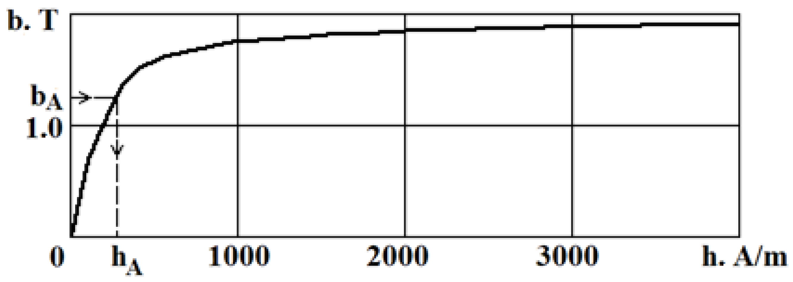
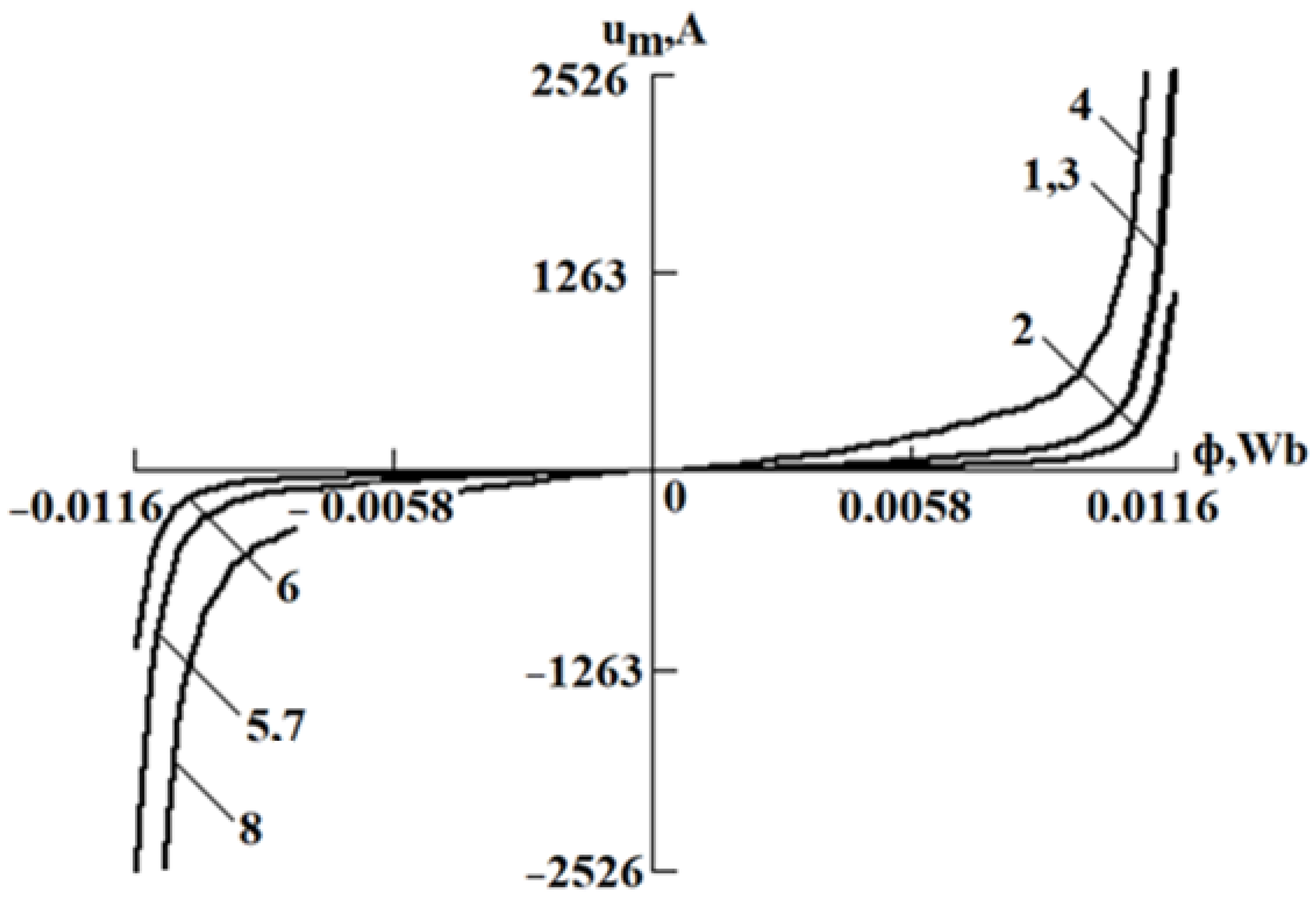
Again, the magnetic field strength,
, in the leg is determined from the magnetization curve shown in
Figure 4 by the calculated
value. This magnetization curve was experimentally derived for the TT-6 transformer.
If the path length of the magnetic flux
in the branch of phase A is considered equal to
, then, taking into account the data in
Figure 1, the magnetic voltage in this branch is
The magnetic voltage,
, is calculated for each
value from the magnetic flux series in the same way, and the dependence,
, is plotted based on the calculation results (curve 1 in
Figure 5). The curves
and
are plotted in the same way (curves 2 and 3). The curves
and
coincide in
Figure 5 because of the same path lengths of the magnetic fluxes
and
.
The calculation of the dependence in general form is complicated since the sizes and configuration of the air gaps and components of the ferromagnetic tank of the transformer should be taken into account. The calculation can be simplified if is assumed to be closed through an additional ferromagnetic branch with the cross-section area S and the length being . In this case, the length, lN, should increase with the transformer power.
The dependence
for the length of
is plotted in
Figure 5 (curve 4). This procedure does not lead to significant errors. The errors are estimated below.
The magnetic fluxes
,
,
, and
can take on negative values; therefore, the dependences
,
,
, and
are shown in
Figure 5 by curves 5–8, which are resulted from rotation of curves 1–4 by 180° around the origin of coordinates.
According to the nodal-pair method [
18,
19], the magnetic voltages
,
,
, and
for the branches of phases A, B, and C and branch N are found from the following equations:
The way of graphical estimation of magnetic fluxes in the legs of a three-phase transformer is shown in
Figure 6, where the curves
,
,
, and
are mirror-reflected about the
axis according to Equation (20), and the curves
,
, and
are shifted along this axis by the values
,
, and
, respectively. The resulted curves,
,
,
, and
, are marked by numbers 1–4 in
Figure 6.
To estimate the fluxes from
Figure 6, line 5 is drawn parallel to the φ axis. It is moved along the magnetic voltage axis until the condition
is satisfied. In this case, the magnetic fluxes in the legs of phases A, B, and C are equal to
,
, and
.
According to [
18,
19], the flux linkage and the inductance in an arbitrary winding are defined as
and
, respectively. Hence, the current values of the self-inductances and mutual inductances of the primary and secondary windings of the transformer in Equations (3) and (4), required for estimation of the flux linkage in the loops by Equation (2), are calculated as
The mutual inductances between the winding phases are
The loop currents are changed to phase currents in
Figure 2, following the equations.
Figure 5 shows that the magnetic flux is low at the length
as compared to the magnetic fluxes in the transformer core legs, and it decreases as
increases. Thus, the choice of the length
within the limits
does not lead to significant errors in the inductances of the transformer.
5. Results and Discussion
The mathematical model developed makes it possible to simulate almost all stationary processes in a healthy three-phase transformer accounting for its nonlinearity. Special software has been created for the model implementation in the TurboBasic V1.1 environment [
20].
The mathematical model was verified by simulating the rated load and no-load modes. The load resistance of the experimental transformer was taken to be equal to 2.5 Ohm in the load mode and infinity in the no-load mode.
It is difficult to visually estimate the adequacy of this mathematical model, for example, through a comparison between the calculated and experimental dependences
of a three-phase transformer. This estimation is much easier to make from a comparison between the harmonic components of these dependencies. To distinguish them, we used the graphical–analytical Fourier-transform method [
18,
19].
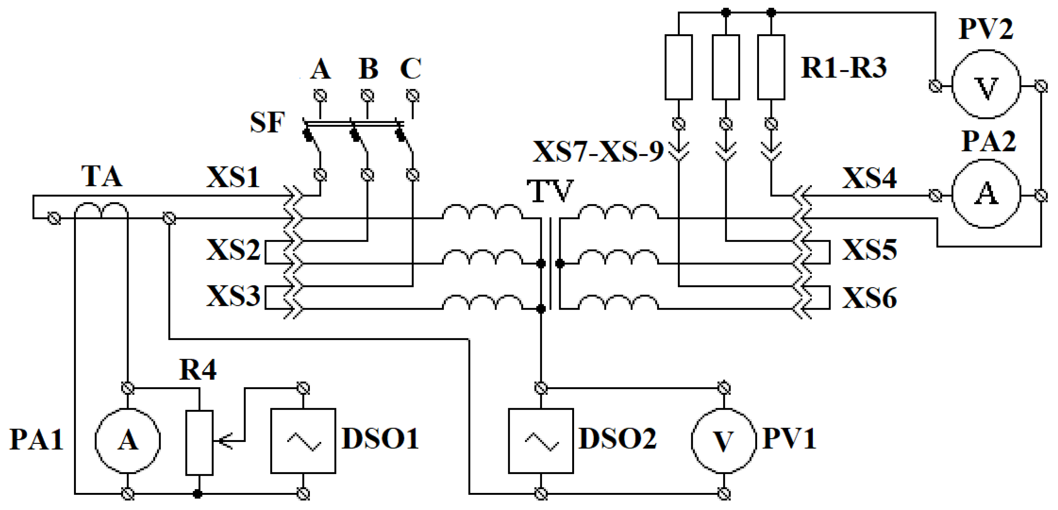
To measure the parameters of the experimental TT-6 transformer and the spectrum of harmonic components in the network voltage and the current in the primary winding of the transformer, we used an experimental setup, the electrical circuit of which is shown in
Figure 7.
As can be seen from
Figure 6, the experimental setup is connected to a three-phase 380 V AC line through circuit breaker SF. The current in the phases of the high- and low-voltage windings of the transformer is measured by ammeters PA1 and PA2. PA1 is a class 0.5 E59 ammeter; it is connected in series with the phases of the primary windings through a class 0.2 I54/1-type current transformer TA with the use of sockets
and plugs with jumpers. This connection of ammeter PA1 makes it possible to use the same device to measure currents in the three phases in turn. This significantly reduces the measurement error.
The spectrum of the harmonic components of currents in the primary winding is recorded with two-beam oscilloscope DSO1. It is based on a personal computer with ELENA-2014 software. The entrance of this oscilloscope is connected to the terminals of ammeter PA1. This provides galvanic isolation of the oscilloscope entrance and the supply line. The voltage at the entrance of DSO1 is controlled with high-ohm resistor R4. The voltage and the harmonic spectrum are controlled with UNI-T UT101 voltmeter PV1 and RIGOL DS1054Z oscilloscope DSO2.
Ammeter PA2 is a class 0.2 D566 device. It is connected in series with the phases of the secondary windings with the use of sockets
and plugs with jumpers. Voltmeter PV2 of YX-360TRD type is connected to the neutral of load, which is resistors R1–R3, and one of the terminals of ammeter PA2. This enables the simultaneous control of current and voltage. The transformer load is commutated with the use of plugs with jumpers and sockets
. The experimental setup is shown in
Figure 8.
The results of the spectral analysis of phase A current during the transformer operation in the no-load and load modes are given in
Table 2 and
Table 3. The comparison between the calculation and experimental results shows the simulation error to be no more than 14% in these operation modes.
One of the reasons for this error is the presence of higher harmonics in the voltage of the supply line during the experiment. Another reason can be the use of numerical methods for estimating the magnetic fluxes in legs.
Nevertheless, the suggested mathematical model of a three-phase transformer enables simulating currents in the transformer windings under steady-state operation modes with accuracy acceptable for the relay protection. Since the requirements for the design of transformers do not depend on their power, there is every reason to believe that the errors will be similar in simulation of the operation of industrial transformers of arbitrary power.
This mathematical model was developed for asymmetrical three-phase transformers with two star-star connected windings without zero grounding. However, it can be used to simulate processes in nonlinear two-winding three-phase transformers with any connection of its windings. In each specific case, the equations of the mathematical model are transformed several times, except for the equations which consider the nonlinearity of the transformer; they remain unchanged.
6. Conclusions
One of the main causes of failures and shortening the service life of two-winding asymmetrical core transformers is the turn-to-turn faults in their windings, which are up to 70–80% of all transformer failures depending on the power and operating conditions.
One of the main ways of decreasing the statistics of these failures and increasing the service life of transformers is the improvement of differential current protections, which is reduced to an increase in their sensitivity to turn-to-turn faults. The operation of these protections is based on the comparison between two electrical quantities with different spectra of currents in phases. Therefore, their sensitivity can be increased by acquiring and taking into account information in the form of the spectrum of these harmonics when choosing the response threshold for differential current protections.
For these purposes, the model with phase coordinates, which is easy for understanding and implementing, can be used. Its differential equations are compiled by the loop current method for phase-to-phase voltages. It uses fourth-order matrices to describe the operation of a three-phase two-winding transformer. Both MATLAB and Turbo Basic environments can be used to implement this mathematical model. However, despite all of its advantages, this model cannot take into account the asymmetry and nonlinearity of a transformer.
In contrast to this model, the mathematical model we suggest makes it possible to consider the asymmetry and nonlinearity of the core of a three-phase transformer by replacing a set of differential equations with a set of linear equations. In the resulted mathematical model, the initial values of its inductances and mutual inductances are determined based on the use of no-load current taking into account the transformer core size, and current values of these parameters are calculated from the currents in the windings and the magnetic fluxes in transformer core legs. The latter are calculated by the nodal-pair method.
The simulation results are presented in the form of harmonics derived from the Fourier transform of the currents, because a visual estimation of the simulation error is quite difficult.
The comparison between the calculation and experimental results showed the error in the harmonic currents in transformer windings to be no higher than 14%. This enables us to estimate the influence of the transformer nonlinearity on the simulation results with acceptable accuracy. We believe that this error is due to the presence of high-order harmonics in the supply voltage during the experiment and the use of numerical method for calculation of these currents.


 ,
, 

