Predicting the Remaining Useful Life of Lithium-Ion Batteries Using 10 Random Data Points and a Flexible Parallel Neural Network

Abstract

Accurate Remaining Useful Life (RUL) prediction of lithium batteries is crucial for enhancing their performance and extending their lifespan. Existing studies focus on continuous or relatively sparse datasets; however, continuous and complete datasets are rarely available in practical applications due to missing or inaccessible data. This study attempts to achieve the prediction of lithium battery RUL using random sparse data from only 10 data points, aligning more closely with practical industrial scenarios. Furthermore, we introduce the application of a Flexible Parallel Neural Network (FPNN) for the first time in predicting the RUL of lithium batteries. By combining these two approaches, our tests on the MIT dataset show that by randomly downsampling 10 points per cycle from 10 cycles, we can reconstruct new meaningful features and achieve a Mean Absolute Percentage Error (MAPE) of 2.36% in predicting the RUL. When the input data are limited to the first 10 cycles using the dataset constructed from random downsampling and the FPNN, the predicted RUL MAPE is 0.75%. The method proposed in this study offers an accurate, adaptable, and comprehensible new solution for predicting the RUL of lithium batteries, paving a new research path in the field of battery health monitoring.

1. Introduction

Lithium batteries, with their significant advantages such as high energy density, eco-friendliness, low self-discharge rate, and long lifespan, have become the preferred choice in emerging energy storage technologies and are widely used across various fields [1,2,3,4,5]. However, the capacity of these batteries gradually diminishes through repeated charging and discharging cycles. The number of cycles a battery undergoes before its capacity falls to 70–80% of its initial capacity is defined as its End of Life (EOL) [6]. Given the long lifespan characteristic of lithium batteries, experimentally determining their lifespan is not only time-consuming but also costly. Therefore, accurately predicting the EOL of batteries is particularly important. Existing studies [7,8] have successfully predicted the EOL, significantly saving time and costs. However, predicting just the EOL is not sufficient; more crucial is the prediction of the Remaining Useful Life (RUL) of the battery, which is vital for providing real-time information about the battery’s current state to users. Moreover, the EOL can be considered a special case of the RUL under initial conditions. Although batteries of the same model may have similar EOLs, their RULs at different stages of use can vary greatly. Batteries at different RUL stages exhibit varying electrochemical characteristics, such as capacity and power. Therefore, compared to the EOL, predicting the RUL is more critical for the maintenance and optimization of battery performance. However, due to the nonlinear changes in batteries during use and the randomness of other conditions, accurately predicting the RUL remains a significant challenge [9].

The methods for predicting the RUL of lithium batteries can be primarily categorized into two types: model-based methods and data-driven approaches. Model-based methods can be further subdivided into electrochemical models [10,11], equivalent circuit models [12], and empirical models [13,14]. For instance, Xing et al. [15] proposed a model combining empirical indices and polynomial regression, which analyzes the degradation trend of batteries throughout their entire cycle life based on experimental data. However, these methods often rely on nonlinear partial differential equations and are highly sensitive to changes in environmental conditions, making the solving process extremely complex [16]. This complexity poses a significant challenge to accurately predicting the RUL. To enhance prediction accuracy, filters [17] can be used for fidelity and noise reduction in model predictions. In 2011, He et al. [18] combined the Dempster–Shafer theory with Particle Filtering (PF) methods to predict battery RUL. In 2013, Miao et al. [19] employed the UPF algorithm based on a degradation model to predict the RUL of lithium-ion batteries, achieving predictions with less than 5% error in the actual RUL.

In 2014, Ng et al. [20] proposed a naive Bayes model to predict battery RUL under varying operational conditions, considering the impacts of different environmental temperatures and discharge currents. Subsequently, data-driven methods based on machine learning began to receive increasing attention. In the field of machine learning, commonly used methods include Support Vector Machine (SVM) [21,22,23,24], Relevance Vector Machine (RVM) [25,26,27], and Gaussian Process Regression (GPR) models [28,29]. Notably, similar to model-based approaches, Relevance Vector Machines are often used in conjunction with other filter algorithms, such as the Kalman Filter (KF) [25], to further enhance prediction accuracy. In 2019, Severson and colleagues [7] successfully trained a simple linear model, achieving an impressive RUL prediction accuracy of up to 9.1%. Additionally, they created the Massachusetts Institute of Technology (MIT) battery dataset, the largest open-source battery dataset to date, providing a valuable resource for the development of neural network models trained on large datasets.

With significant advancements in computational capabilities, neural networks have garnered widespread attention in the field of lithium battery RUL prediction [30,31]. Ren et al. [31] achieved an accuracy of up to 88.2% in RUL prediction using 21 extracted features and a deep neural network, particularly excelling when a larger number of input cycles were involved. This represented a notable improvement over traditional methods such as linear regression and SVM. In handling electrochemical sequence data, Recurrent Neural Networks (RNNs) [32] have shown unique advantages. Long Short-Term Memory (LSTM) networks, a variant of RNNs, are capable of handling variable-dimensional inputs and optimizing parameters through prior information, demonstrating significant accuracy in long-term RUL predictions [33,34,35,36,37]. Zhang et al. [36] used an LSTM network to predict the RUL from lithium-ion battery data, effectively avoiding the vanishing gradient problem common in traditional RNNs. Additionally, Convolutional Neural Networks (CNNs), known for extracting local spatial features in electrochemistry, have also been applied in RUL prediction [38]. Some studies [33,39,40,41] combined CNNs with RNNs and their variants to further enhance the accuracy of RUL predictions. However, due to the reliance of RNNs and their variants on previous moment data in the computation process, parallel computing is challenging. To address this, Chen et al. [42] attempted to combine a 1D CNN with a 2D CNN and used LSTM to capture temporal information, achieving a RUL prediction error of only 3.37% using just 50 cycles. Yang, Y. [43] completely abandoned LSTM and, by combining a three-dimensional CNN (3D CNN) with a 2D CNN, achieved an RUL prediction error of 3.55% using only 10 cycles of charging data. Furthermore, considering the discontinuity of experimental data in practical applications, Zhang et al. [44] used only 20% of sparse charging data from 10 cycles for RUL prediction, yet still maintained the error within 4.15%.

However, in practical applications, obtaining continuous 20% of charging data is often challenging. In light of this, our study adopts a novel data processing method: each sample contains charging data from 10 cycles, but only 10 points are randomly sampled from each cycle, forming a new dataset. Jiang et al. [45] designed the Flexible Parallel Neural Network (FPNN), which achieved state-of-the-art (SOTA) results in the early prediction of battery life. In this paper, we input these randomly sampled 10 points of data into the FPNN for battery RUL prediction.

The main contributions of this paper can be summarized as follows:

(1) Super-Sparse Data: This study is the first to use super-sparse random charging data consisting of only 10 points for lithium battery RUL prediction, better aligning with real-world production environments.

(2) Successful Application of FPNN in RUL Prediction: FPNN is an excellent interpretable model, and this study reaffirms its effectiveness. The combination of sparse data with FPNN enables our research to reach a new state-of-the-art level in RUL prediction.

The structure of the paper is arranged as follows. Section 2 details the MIT dataset, including its composition and charging process data. Section 3 describes the method of data sparsification and the evaluation metrics for model prediction performance. Section 4 presents the experimental results and in-depth analysis. It first introduces the performance evaluation of the presented method, compares it with existing methods, conducts ablation experiments, and concludes the paper with a summary and conclusions.

2. Datasets

In this study, we utilized the MIT dataset [7]. Since the basic information of the dataset is similar to that in previous studies, it is not elaborated here in detail. In each charging cycle of the MIT dataset, the charging capacity gradually increases with the charging process until it reaches the maximum capacity, indicating the completion of charging. This dataset consists of three ‘.mat’ files, representing battery data from three different batches. As shown in Figure 1, data from 40 batteries in the third batch are displayed, whereas data from the other two batches are presented in the appendix in Figure A1 and Figure A2. Different batteries have different cycle lifespans, and the charging completion times also vary at different cycle stages for the same battery. To ensure consistent access to charging process data, this study calculated the average index at which data points reach the charging completion time. 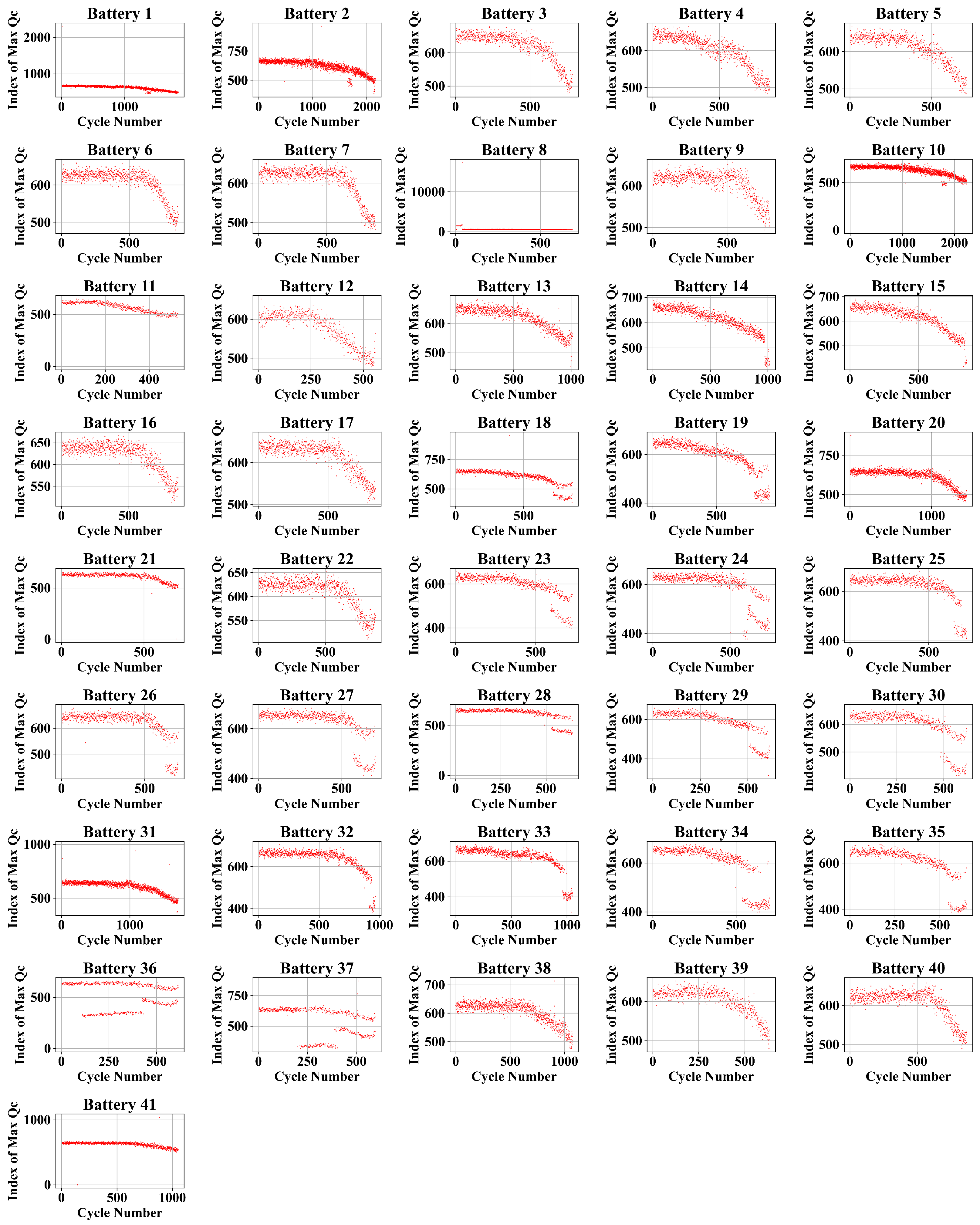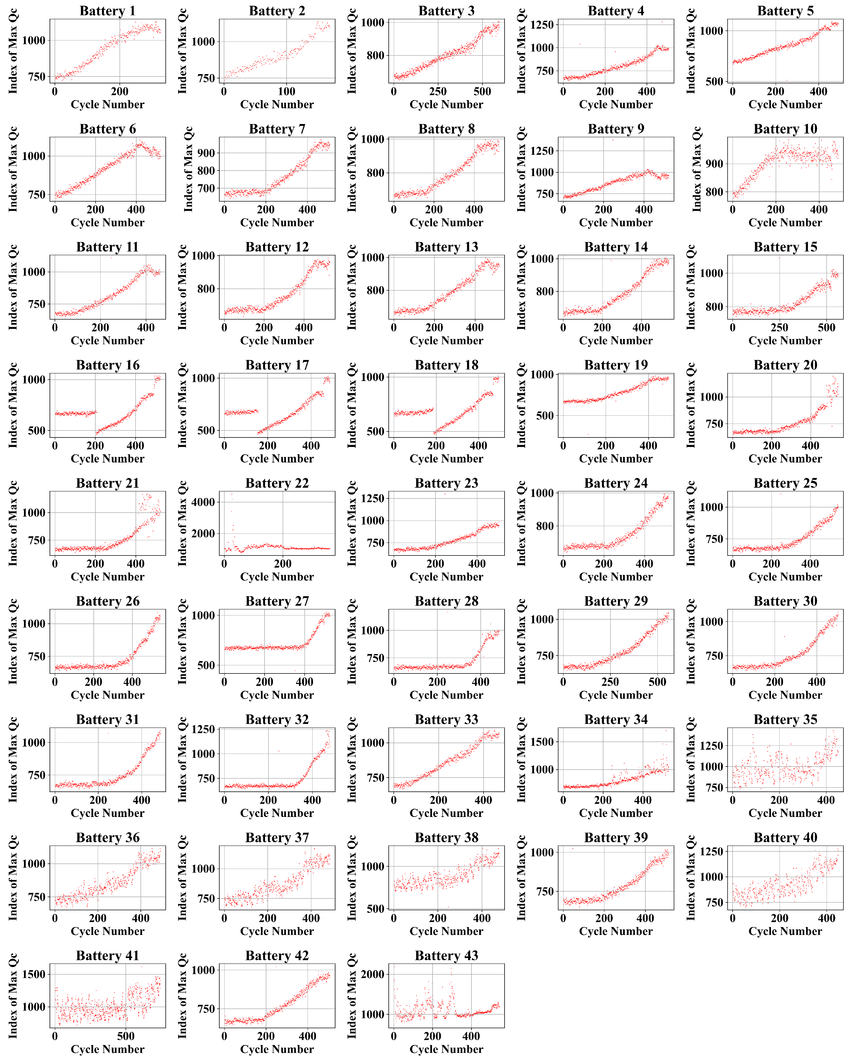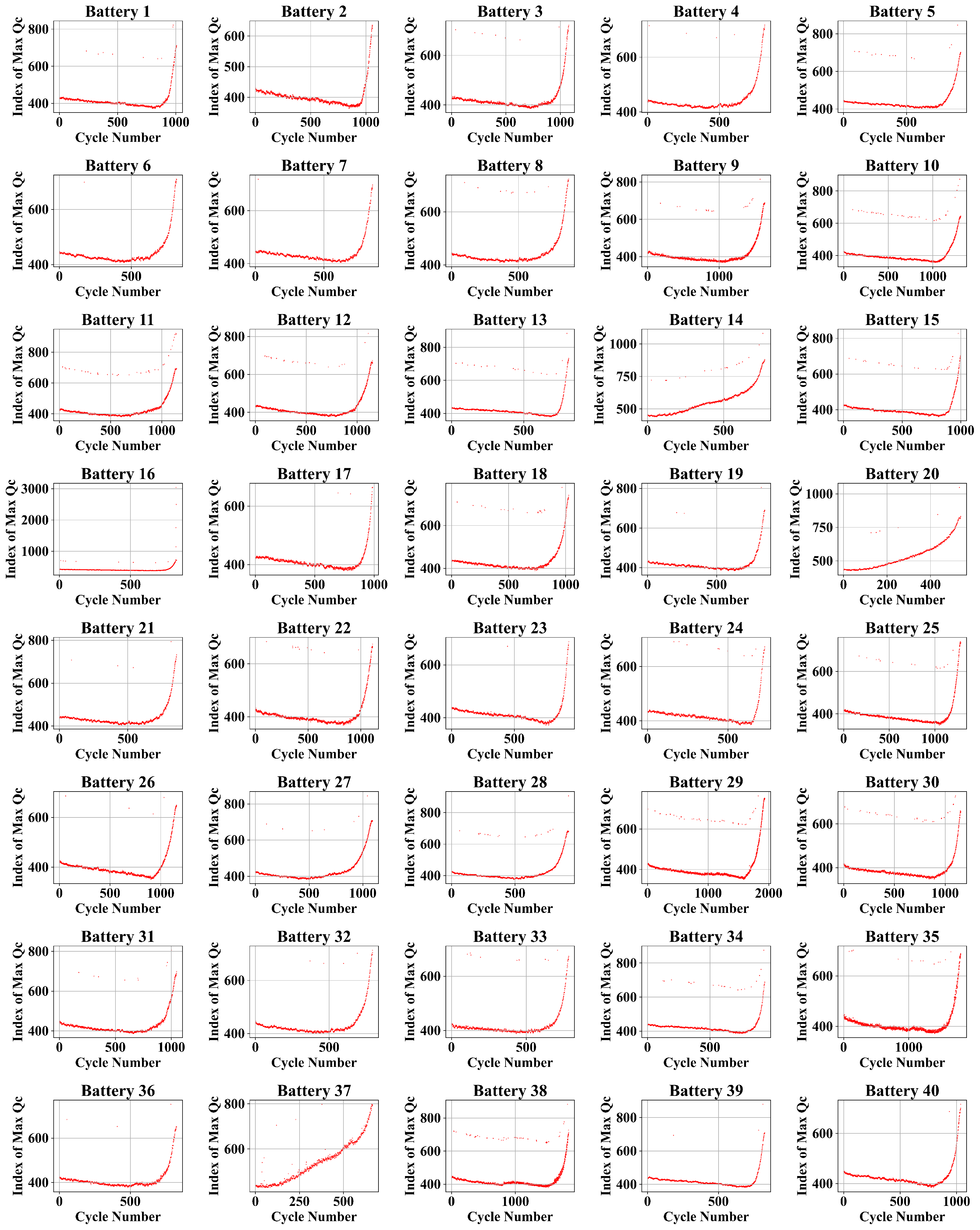Subsequently, data from the first 400 points were extracted for analysis.

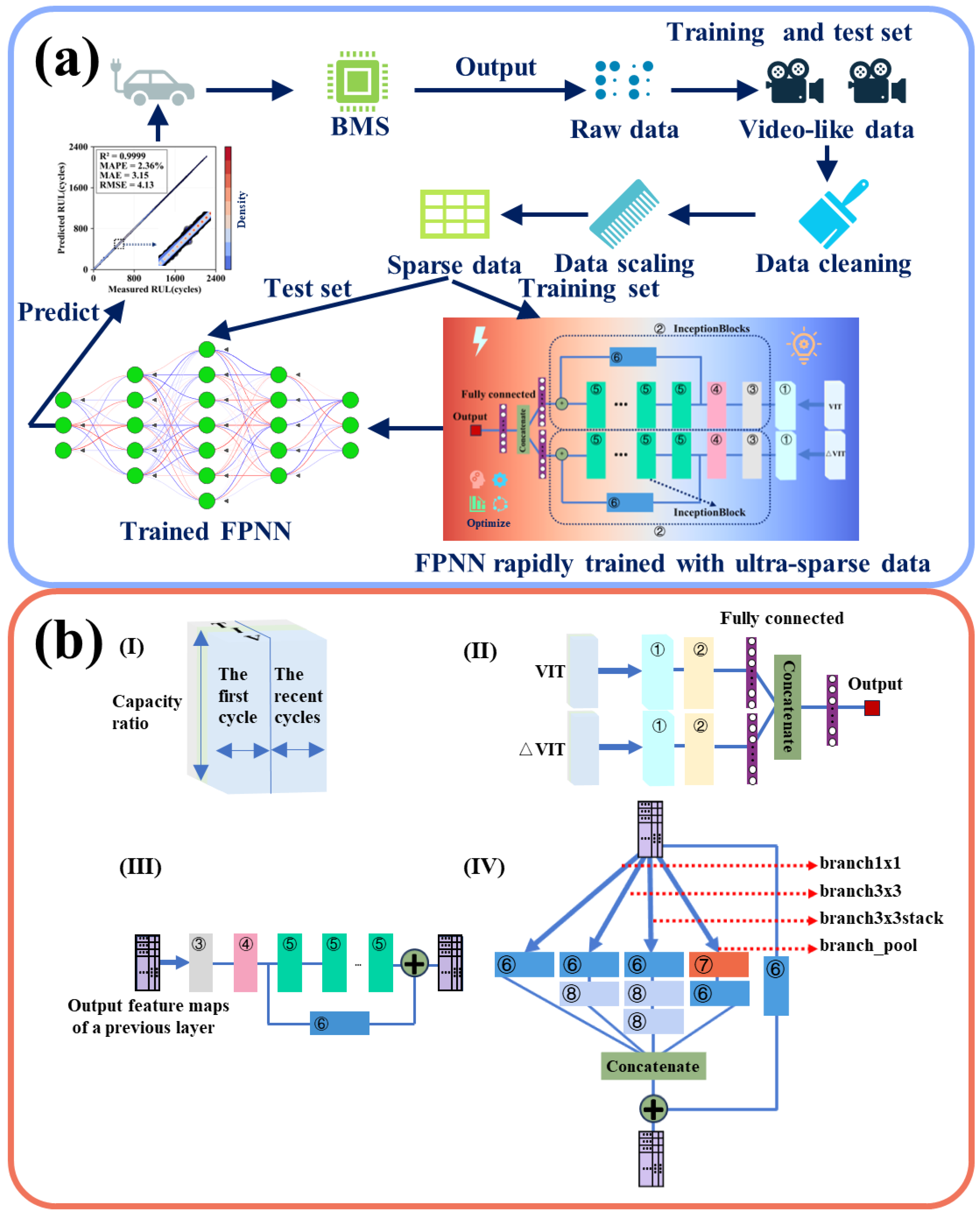
3. Methodology

Following the comprehensive introduction of the dataset in the previous section, this section further elaborates on the overall workflow for predicting the RUL of batteries. As illustrated in Figure 2, the process begins with the Battery Management System (BMS), whose primary responsibility is to collect data during battery operation. These raw data are then subjected to a series of preprocessing steps, transforming them into a video-like format to enhance their processability. Subsequently, the super-sparse data obtained from the randomly sampled 10 data points are fed into the FPNN for model training and prediction tasks. The hyperparameters of the FPNN model are determined through Bayesian optimization algorithms, and except for the varying number of downsampled data points, the other hyperparameters remain consistent across the different RUL prediction tasks. Finally, the model’s predictions are presented through a meticulously designed data visualization tool.

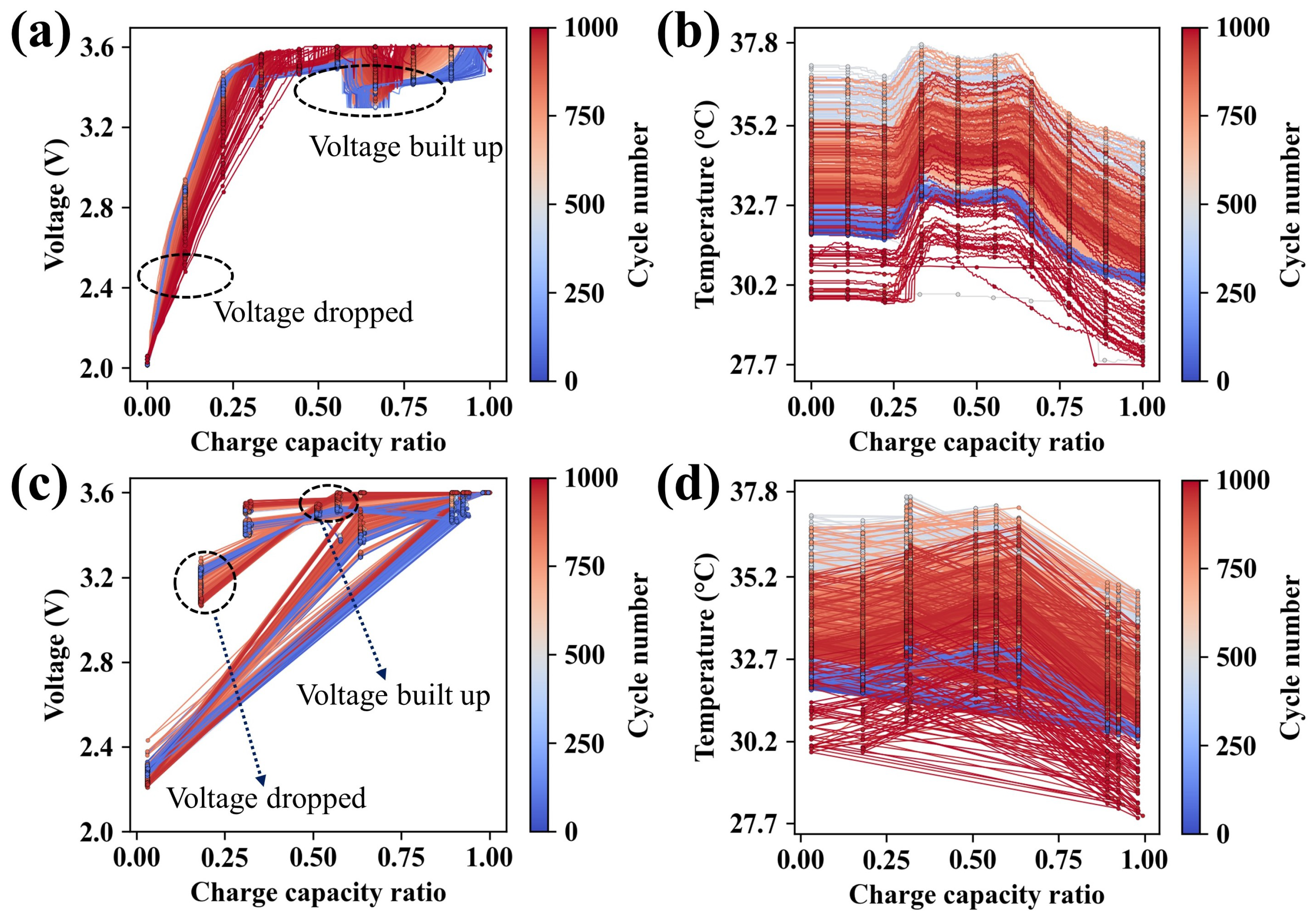
3.1. Data Preprocessing

Prior to inputting data into the model, a series of preprocessing steps is required, similar to those described in Jiang et al. [45]. However, unlike the sample cycle numbers selected in previous studies (the 1st cycle and its adjacent 3 cycles), each sample in this study consisted of the first 5 cycles of the battery and its most recent 5 cycles. This method of sample selection aimed to increase the similarity between samples, consistent with the settings used in other studies [43,44].

3.2. Data Sparsification

Following data preprocessing, the data underwent sparse processing treatment. As shown in Figure 3a,b, uniform downsampling of 10 points per cycle was performed, ensuring that the contour of the features was not lost. Considering that uniform sampling is relatively rare in real-life scenarios, random sampling better aligns with actual production conditions. As depicted in Figure 3c,d, by randomly sampling 10 points from each cycle’s data, new features corresponding to each cycle number were reconstructed. Whether through uniform or random sampling, the newly generated electrochemical features changed as the cycles progressed, providing a solid foundation for mapping the RUL. Furthermore, the downsampling operation significantly reduced hardware requirements and accelerated the speed of model training and inference.

3.3. Hyperparameter Optimization

In this study, the Bayesian optimization algorithm [46] was employed to precisely determine the hyperparameters of the FPNN model. By utilizing Gaussian Process Regression as a surrogate model, Bayesian optimization not only facilitated value prediction but also provided confidence intervals, effectively balancing exploration and exploitation. As a key hyperparameter, the number of InceptionBlocks (NOI) in the FPNN for the different RUL tasks was uniformly set to 3 to control the variables, allowing for a more accurate comparison of the impact of different sampling methods on the RUL prediction tasks. In all cases, new individual samples were composed of data from 10 cycles, with 10 points randomly sampled from each cycle of each sample after preliminary preprocessing to form a new dataset. In these datasets, although each sample consisted of data from 10 cycles, there were only 10 data points per cycle, significantly speeding up the training process. Under these conditions, an optimal hyperparameter search for the FPNN was conducted. Subsequently, in the other RUL prediction tasks, the hyperparameter settings remained the same to ensure the accuracy of the study. Except for the number of downsampled data points, all hyperparameters were consistent across early and non-early predictions, as well as random and uniform sampling. This methodical strategy was crucial for accurately assessing the impact of the number of downsampled data points, ensuring the effectiveness and comparability of the findings.

The definition of the RUL follows Equation (1), where $N_{EOL}$ represents the cycle life of the battery and $N_{ECL}$ represents the number of cycles the battery has already completed. RUL represents the difference between these two values and is the target value to be predicted.

$$RUL=N_{EOL}-N_{ECL}$$

(1)

To comprehensively evaluate the predictive performance of the model, this study selected the Mean Absolute Percentage Error (MAPE), Mean Absolute Error (MAE), and Root-Mean-Square Error (RMSE) as the evaluation metrics. The corresponding mathematical expressions are given in Equations (2)–(4):

$$\mathrm{MAPE}=\frac{100\%}{n}\sum _{i=1}^n\left|\frac{y_i-{\widehat{y}}_i}{y_i}\right|$$

(2)

$$\mathrm{MAE}=\frac{1}{n}\sum _{i=1}^n\left|y_i-{\widehat{y}}_i\right|$$

(3)

$$\mathrm{RMSE}=\sqrt{\frac{1}{n}\sum _{i=1}^n{\left(y_i-{\widehat{y}}_i\right)}^2}$$

(4)

where n is the total number of samples, $y_i$ is the actual value of the i-th sample, and ${\widehat{y}}_i$ is the predicted value of the i-th sample.

4. Results and Discussion

Each individual sample was composed of data from 10 cycles. When using data from the first 10 cycles as the sample, according to Equation (1), $N_{EOL}$ equals the RUL plus 10, representing the cycle life of the battery. Therefore, in this case, the study actually involved the early prediction of the battery’s cycle life using early data, aligning with the objectives of previous research. Consequently, this section focuses on the early prediction of the RUL. In the other scenarios, to predict the RUL of the battery at any given time point, the test set consisted of complete data from all cycles, where each individual sample was composed of data from 10 cycles. Although the randomly sampled data more closely reflect real production conditions, to provide a comparative baseline, this paper also considered datasets with uniformly sampled data for comparative analysis alongside those with randomly sampled data.

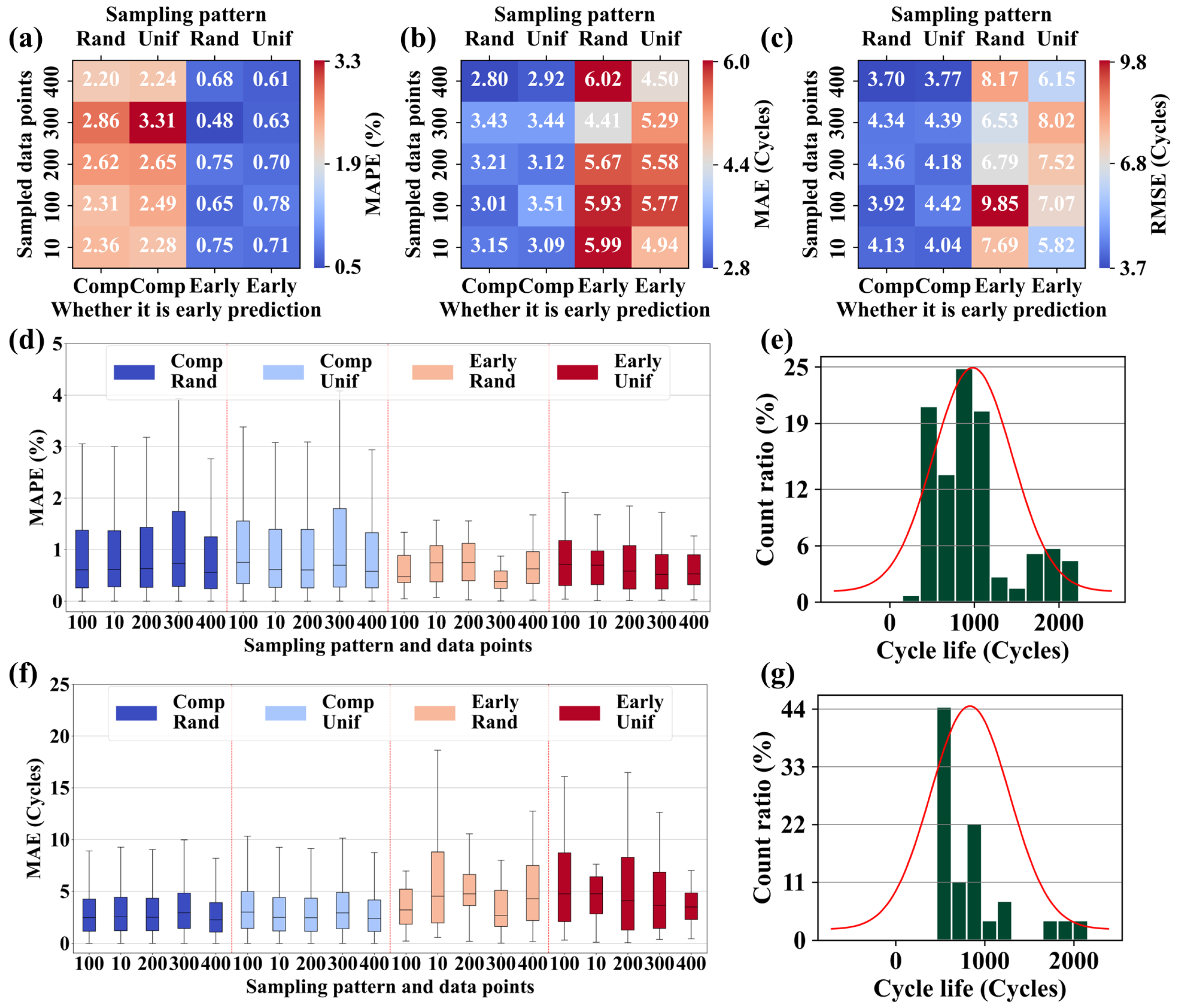
4.1. Predictive Performance under Different Conditions

Figure 4a–c depict heatmaps of various error metrics. Notably, for early predictions, the MAPE values were significantly lower compared to non-early predictions. This result even surpassed previous studies, where the accuracy for early predictions remained below 1% across different sampling data points. By adding the predicted RUL to 10, the cycle life of the battery could be obtained. This phenomenon can be attributed to the fact that, unlike Jiang et al. [45], who included samples with only 4 cycles of data, the samples in this study contained data from 10 cycles, providing richer and more specific electrochemical information within each sample. However, although the samples in this study contained data from 10 cycles, the MAPE for early predictions was smaller than that for non-early predictions, which can be explained by Equation (2). For samples from the same battery, the actual RUL labels for early predictions were larger, whereas those for non-early predictions were smaller. Since the actual RUL label is in the denominator, the MAPE for early predictions was smaller. This is validated in Figure 4b–c, where it can be seen that for error metrics that do not require normalization, non-early predictions were more accurate, with lower absolute errors, aligning with the common consensus that early predictions were more challenging to model accurately compared to non-early predictions. Considering that the RMSE and MAE exhibited similar trends, only the box plots of the MAPE and MAE are shown in Figure 4d. The MAPE for non-early predictions exhibited greater variability, possibly because the MAPE for non-early predictions was larger than that for early predictions, leading to increased differences in extreme values of the MAPE and a broader range of data distribution covered by different samples. Since the MAE for non-early predictions was smaller than that for early predictions, the distribution of the MAE in Figure 4f shows an opposite trend to the distribution of the MAPE in Figure 4d.

Subsequently, Figure 4e,g display the distribution of the cycle life for the non-early and early prediction samples, respectively. Given that the entire MIT dataset comprised 124 batteries, there could be up to 124 different cycle life values, meaning that all samples from the same battery share one cycle life. Consistent with Jiang et al. [45], the training and test sets were divided in a 94:30 ratio. Despite the large number of RUL samples overall, there were relatively fewer samples for early predictions, which may account for the higher non-normalized error metrics (MAE, RMSE) observed for early predictions. Conversely, there were more samples for non-early predictions, covering almost all 124 possible cycle life values. With the same number of data points, random and uniform sampling each exhibited distinct advantages, albeit with minor differences. When other conditions remained constant, various types of errors showed slight fluctuations with the changes in the number of sampling points, possibly because different total numbers of data points could still clearly describe the framework texture of features.

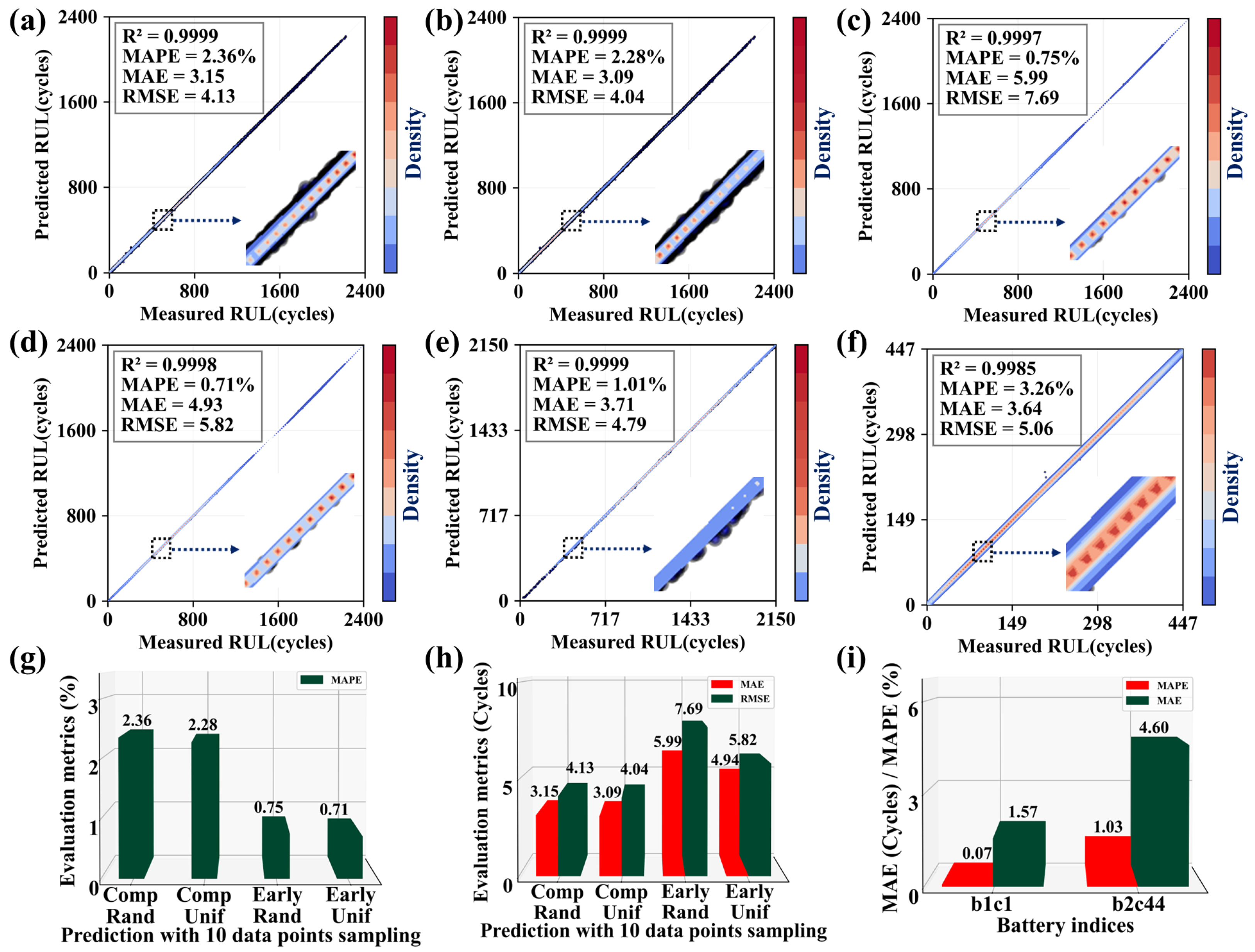
4.2. Predictive Performance under 10 Data Points

Considering the practical value of using 10 data points, this section focuses on the prediction scenarios when sampling 10 data points. Figure 5a,b show the non-early prediction RUL scenarios for random and uniform sampling, respectively. Overall, the difference between the two is minimal, but uniform sampling has a slight edge in this context. Figure 5c,d display the early prediction RUL scenarios for random and uniform sampling, where again, the overall difference is small, but uniform sampling maintains a slight advantage. Figure 5e,f illustrate the prediction scenarios for individual batteries “b1c1” and “b2c44” under random sampling datasets. Here, we selected single battery data representing the extreme cases of maximum and minimum cycle lives for RUL prediction. The selection of individual batteries in this study differs from previous research, as early samples from those batteries were not randomly allocated to the test set, preventing early RUL prediction for individual batteries. The early prediction scenarios for random sampling of “b1c1” and “b2c44” batteries are shown in Figure 5i, demonstrating that even under extreme conditions, the data processing method in this study combined with the FPNN still exhibits strong robustness. Additionally, the scenarios of early and non-early RUL predictions with 10-point sampling are more clearly presented in Figure 5g,h, with the conclusions consistent with those of the previous subsection.

Finally,

Table 1. RUL prediction using datasets formed by randomly sampling different data points.

Complete/Early	Points	MAPE (%)	MAE (Cycles)	RMSE (Cycles)
Complete	10	2.36	3.15	4.13
	100	2.31	3.01	3.92
	200	2.62	3.21	4.36
	300	2.86	3.43	4.34
	400	2.20	2.80	3.70
Early	10	0.75	5.99	7.69
	100	0.65	5.93	9.85
	200	0.75	5.67	6.79
	300	0.48	4.41	6.53
	400	0.68	6.02	8.17

provides a detailed list of the specific numerical results for early and non-early RUL predictions using datasets with different numbers of data points from random sampling. Our method is compared with other published methods in

Table 2. RUL prediction from other published research methods.

Methods	MAPE (%)	MAE (Cycles)	RMSE (Cycles)	Requirements for Input Data
Linear model [7]	9.1	—	—	The dense data of the 100 cycles
HPR CNN [44]	5.16	46.69	64.52	20% sparse charging data from the first 10 cycles
HPR CNN [44]	4.15	16.09	27.47	20% sparse charging data from 10 cycles
HCNN [43]	3.55	9	11	Dense charging data of the 60 cycles
TOP-Net [42]	3.37	8	11	The dense data of the 50 cycles
Proposed method	2.36	3.15	4.13	10 random charging points from each of 10 cycles
Proposed method	0.75	5.99	7.69	10 random charging points from each of the first 10 cycles

. The comparison reveals that the novel data processing approach used in this study combined with the FPNN demonstrates exceptional performance in predicting the RUL, successfully achieving SOTA level.

4.3. Ablation Experiments

To validate the effectiveness of this study, this section presents comprehensive data from ablation experiments conducted for various scenarios. Detailed tabular data can be found in Appendix A, specifically in

Table A1. The results of non-early RUL predictions using datasets formed by sampled data points.

Sampling Mode	Points	Detach	MAPE (%)	MAE (Cycles)	RMSE (Cycles)
Random sampling	10	None	2.36	3.15	4.13
	10	Initial layers	3.23	3.87	5.06
	10	Residual	2.20	3.12	4.04
	10	3D conv	3.88	5.61	7.75
	10	1 block	2.54	3.72	4.83
	10	2 blocks	4.00	4.38	5.62
Random sampling	10	3 blocks	2.68	3.72	5.02
	10	A branch	99.86	484.65	619.75
	100	None	2.31	3.01	3.92
	100	Initial layers	6.07	7.21	8.87
	100	Residual	2.39	3.16	4.08
	100	3D conv	4.46	5.61	7.32
	100	1 block	3.37	4.73	6.01
	100	2 blocks	4.37	5.37	6.51
	100	3 blocks	11.17	13.62	14.35
	100	A branch	99.84	484.56	619.63
	200	None	2.62	3.21	4.36
	200	Initial layers	NaN	NaN	NaN
	200	Residual	1.87	2.69	3.45
	200	3D conv	4.36	5.92	7.44
	200	1 block	2.7	3.99	4.85
	200	2 blocks	2.56	3.46	4.45
	200	3 blocks	7.07	7.43	8.75
	200	A branch	99.85	484.58	619.65
	300	None	2.86	3.43	4.34
	300	Initial layers	NaN	NaN	NaN
	300	Residual	2.24	2.87	3.84
	300	3D conv	5.07	7.58	9.07
	300	1 block	2.76	3.32	4.32
	300	2 blocks	2.59	3.28	4.29
	300	3 blocks	3.99	5.43	6.8
	300	A branch	99.84	484.57	619.63
	400	None	2.2	2.8	3.7
	400	Initial layers	NaN	NaN	NaN
	400	Residual	2.07	3.11	3.96
	400	3D conv	3.75	5.48	7
	400	1 block	2.88	3.5	4.61
	400	2 blocks	5.42	8.24	10.29
	400	3 blocks	6.47	7.12	8.66
	400	A branch	99.85	484.63	619.72
Uniform sampling	10	None	2.28	3.09	4.04
	10	Initial layers	2.80	3.40	4.50
	10	Residual	2.52	3.22	4.50
	10	3D conv	4.40	6.06	8.24
	10	1 block	2.48	2.97	3.98
	10	2 blocks	2.63	3.31	4.39
	10	3 blocks	3.44	3.91	5.09
	10	A branch	99.86	484.67	619.77
	100	None	2.49	3.51	4.42
	100	Initial layers	4.53	4.93	6.17
	100	Residual	2.13	2.96	3.8
	100	3D conv	3.95	4.96	6.56
	100	1 block	2.6	4.05	5.2
	100	2 blocks	2.48	3.23	4.21
	100	3 blocks	4.71	7	8.66
	100	A branch	99.83	484.53	619.6
	200	None	2.65	3.12	4.18
	200	Initial layers	NaN	NaN	NaN
	200	Residual	1.92	2.48	3.27
	200	3D conv	3.77	5.2	6.77
	200	1 block	2.42	2.97	3.95
	200	2 blocks	2.53	3.15	4.16
	200	3 blocks	5.84	6.39	7.82
	200	A branch	99.84	484.58	619.64
	300	None	3.31	3.44	4.39
	300	Initial layers	NaN	NaN	NaN
	300	Residual	2.07	2.83	3.77
	300	3D conv	3.54	5.05	6.64
	300	1 block	3.65	4.04	5.12
	300	2 blocks	2.98	3.51	4.55
	300	3 blocks	3.42	5.08	6.53
	300	A branch	99.84	484.56	619.61
	400	None	2.24	2.92	3.77
	400	Initial layers	NaN	NaN	NaN
Uniform sampling	400	Residual	2.29	2.72	3.56
	400	3D conv	3.35	4.51	6.01
	400	1 block	2.72	3.38	4.48
	400	2 blocks	3.78	5.62	7.15
	400	3 blocks	6.75	8.75	10.17
	400	A branch	99.85	484.66	619.74

Note: (1) ‘NaN’ indicates missing data because in these scenarios, after removing the initialization layer, the model consumed excessive GPU memory during training, preventing these experiments from being conducted. (2) ‘A branch’ refers to the differential feature branch removed from the dual-stream network.

(non-early RUL predictions) and

Table A2. The results of early RUL predictions using datasets formed by sampled data points.

Sampling Mode	Points	Detach	MAPE (%)	MAE (Cycles)	RMSE (Cycles)
Random sampling	10	None	0.75	5.99	7.69
	10	Initial layers	0.70	5.57	7.62
	10	Residual	0.76	5.41	6.24
	10	3D conv	1.17	9.86	13.38
	10	1 block	0.52	3.50	4.33
	10	2 blocks	0.91	6.21	6.96
	10	3 blocks	0.90	7.80	10.89
	10	A branch	99.60	820.09	931.36
	100	None	0.65	5.93	9.85
	100	Initial layers	1.22	9.97	12.93
	100	Residual	0.74	5.61	7.76
	100	3D conv	0.86	6.84	10.31
	100	1 block	0.83	7.04	9.96
	100	2 blocks	1.08	8.49	10.45
	100	3 blocks	1.7	11.44	12.41
	100	A branch	99.58	819.93	932.21
	200	None	0.75	5.67	6.79
	200	Initial layers	NaN	NaN	NaN
	200	Residual	0.57	4.49	6.58
	200	3D conv	1.2	9.8	14.38
	200	1 block	0.62	4.5	5.49
	200	2 blocks	0.97	7.33	9.27
	200	3 blocks	1.55	11.37	13.39
	200	A branch	99.58	819.95	931.22
	300	None	0.48	4.41	6.53
	300	Initial layers	NaN	NaN	NaN
	300	Residual	0.64	4.29	5.67
	300	3D conv	1.6	12.54	15.29
	300	1 block	0.78	6.43	8.97
	300	2 blocks	0.7	5.99	8.02
	300	3 blocks	0.86	7.5	11.64
	300	A branch	99.58	819.93	931.19
	400	None	0.68	6.02	8.17
	400	Initial layers	NaN	NaN	NaN
	400	Residual	0.56	4.48	6.48
	400	3D conv	1.23	9.4	12.16
	400	1 block	0.74	6.51	9.82
	400	2 blocks	1.37	12.49	17.37
	400	3 blocks	1.08	8.45	11.23
	400	A branch	99.6	820.04	931.34
Uniform sampling	10	None	0.71	4.94	5.82
	10	Initial layers	0.62	4.69	6.22
	10	Residual	0.51	3.63	4.25
	10	3D conv	1.30	10.96	16.38
	10	1 block	0.69	4.91	5.82
	10	2 blocks	0.52	3.50	4.54
	10	3 blocks	0.76	6.77	10.16
	10	A branch	99.60	820.10	931.40
	100	None	0.78	5.77	7.07
	100	Initial layers	0.75	6.79	9.49
	100	Residual	0.66	5.3	7.64
Uniform sampling	100	3D conv	1.34	10.46	15.11
	100	1 block	1	8.49	11.73
	100	2 blocks	0.76	6.92	10.09
	100	3 blocks	0.77	5.77	7.76
	100	A branch	99.58	819.9	931.19
	200	None	0.7	5.58	7.52
	200	Initial layers	NaN	NaN	NaN
	200	Residual	0.71	5.28	7.36
	200	3D conv	0.94	7.73	11.04
	200	1 block	0.89	6.74	8.93
	200	2 blocks	0.87	7.77	10.85
	200	3 blocks	1.01	8.93	12.87
	200	A branch	99.58	819.94	931.22
	300	None	0.63	5.29	8.02
	300	Initial layers	NaN	NaN	NaN
	300	Residual	0.66	4.8	6.08
	300	3D conv	1.42	11.78	16.94
	300	1 block	0.66	5.54	8.09
	300	2 blocks	0.6	5.3	8.41
	300	3 blocks	1.2	10.16	12.86
	300	A branch	99.58	819.93	931.19
	400	None	0.61	4.5	6.15
	400	Initial layers	NaN	NaN	NaN
	400	Residual	0.63	4.76	6.36
	400	3D conv	1.08	9.03	14.65
	400	1 block	0.74	6.28	9.73
	400	2 blocks	0.97	9.77	15.15
	400	3 blocks	1.21	8.06	9.55
	400	A branch	99.72	820.65	931.67

Note: (1) ‘NaN’ indicates missing data because in these scenarios, after removing the initialization layer, the model consumed excessive GPU memory during training, preventing these experiments from being conducted. (2) ‘A branch’ refers to the differential feature branch removed from the dual-stream network.

(early RUL predictions). Figure 6a–c display heatmaps of the ablation experiments under all conditions. Given the significant differences in data extremes, a simple mathematical transformation was applied to the original data, namely $y=log(1+x)$, where x represents the original error evaluation metric and y is the processed evaluation metric, which is also the value shown in the figures. ’NaN’ is used to indicate missing data because in these scenarios, after removing the initialization layer, the model consumed excessive GPU memory during training, preventing these experiments from being conducted.

In these experiments, the logarithmic MAPE for early predictions was generally smaller, whereas the MAPE for non-early predictions was larger. Conversely, other non-normalized error metrics like the MAE and RMSE showed the opposite trend. This is consistent with the patterns observed in previous prediction results. It is evident that removing different components of the FPNN model impacted its RUL prediction capability in the various scenarios. Since previous research has indicated that setting the NOI to 3 performs well under different conditions, the NOI in this study was also set to 3.

In this study, special attention was given to the MAPE, a normalized metric, particularly for non-early prediction scenarios. When randomly selecting 10 data points and sequentially removing each layer in the FPNN, it was observed that the accuracy of the FPNN generally decreased. However, interestingly, when the residual was removed, the accuracy slightly improved. This suggests that under the current data distribution, residual connections might have had a minor adverse effect. However, it is important to note that removing residual connections did not always produce adverse effects in other scenarios with different numbers of data points and sampling patterns; sometimes, it even enhanced accuracy. The initial layers, differential feature branch, and 3D conv consistently contributed positively to the model, and their removal led to a decline in model performance. Particularly, the differential feature branch had the most significant impact on the FPNN’s performance, with its removal greatly diminishing the FPNN’s capabilities. The initial NOI in the current model was set to 3. For non-early predictions with 300 randomly sampled data points, removing one InceptionBlock slightly improved the FPNN’s accuracy, and the same was observed for non-early predictions with 200 uniformly sampled data points. However, in other scenarios, the FPNN’s performance typically worsened. When removing two InceptionBlocks, there was a slight improvement in accuracy for non-early predictions with 200 and 300 randomly sampled data points, as well as for 200 uniformly sampled data points. Yet, when all three InceptionBlocks were removed, the FPNN’s performance significantly declined across all non-early prediction scenarios.

In the case of early predictions, the situation changed slightly. Removing the initial layers only led to adverse results when sampling 100 data points, whereas in other scenarios with available data, the FPNN’s performance slightly improved. Similar to non-early predictions, removing the residual sometimes had beneficial effects and sometimes the opposite. The differential feature branch and 3D conv were consistently beneficial. With the initial NOI set to 3, removing one InceptionBlock generally led to a decrease in the FPNN’s performance, but there were improvements in scenarios with 10 and 100 randomly sampled points and 10 uniformly sampled points. When removing two InceptionBlocks, the FPNN’s performance generally declined, but there were improvements in scenarios with 10, 100, and 300 uniformly sampled points. Finally, when all three InceptionBlocks were removed, the FPNN’s performance generally declined, but there was an improvement in the scenario with 100 uniformly sampled points.

Given the practical significance of sampling 10 data points, Figure 6d presents bar graphs of the MAPE, MAE, and RMSE when sampling 10 data points. As previously mentioned, the differential feature branch is crucial, a fact that is reaffirmed in this chart. The roles of the other layers are also quite evident, with the unaltered FPNN consistently performing well under various conditions. Certain layers, particularly the residual connections and NOI, had mixed effects on the FPNN’s performance. However, this also confirms previous research findings [45] that adapting the NOI to suit different conditions can fully harness the potential of the FPNN.

Finally, for detailed information on the ablation experiments conducted for RUL prediction using datasets with 10 randomly sampled data points, please refer to

Table 3. Ablation experiments using a dataset formed by randomly sampling 10 data points.

Complete/Early	Detach	MAPE (%)	MAE (Cycles)	RMSE (Cycles)
Complete	None	2.36	3.15	4.13
	Initial layers	3.23	3.87	5.06
	Residual	2.20	3.12	4.04
	3D conv	3.88	5.61	7.75
	1 block	2.54	3.72	4.83
	2 blocks	4.00	4.38	5.62
	3 blocks	2.68	3.72	5.02
	A branch	99.86	484.65	619.75
Early	None	0.75	5.99	7.69
	Initial layers	0.70	5.57	7.62
	Residual	0.76	5.41	6.24
	3D conv	1.17	9.86	13.38
	1 block	0.52	3.50	4.33
	2 blocks	0.91	6.21	6.96
	3 blocks	0.90	7.80	10.89
	A branch	99.60	820.09	931.36

.

5. Conclusions

This paper successfully integrates the FPNN model with the super-sparse random sampling data processing technique for precise prediction of battery RUL on the MIT dataset, demonstrating outstanding predictive accuracy. With random downsampling of 10 data points per cycle, the model reconstructed new, meaningful features, achieving an MAPE of 2.36% for RUL prediction. When the input data were limited to the first 10 cycles, the predicted RUL MAPE dropped to 0.75%. To comprehensively assess the proposed technique, we also conducted comparative experiments with uniform sampling. The results showed with both random sampling and uniform downsampling, the error of FPNN prediction is very low, and the corresponding variance is very small, reaching the current SOTA level. This indicates that even super-sparse random data can effectively establish the mapping relationship between features and labels. Furthermore, through ablation experiments, this study further confirmed the importance and necessity of each component in the FPNN architecture. Given the commonality between RUL tasks and other machine learning tasks in the battery domain, the novel sparse data processing method adopted in this study signifies its huge potential for broader application in the battery field.

References

- Shchegolkov, A.V.; Komarov, F.F.; Lipkin, M.S.; Milchanin, O.V.; Parfimovich, I.D.; Shchegolkov, A.V.; Semenkova, A.V.; Velichko, A.V.; Chebotov, K.D.; Nokhaeva, V.A. Synthesis and study of cathode materials based on carbon nanotubes for lithium-ion batteries. Inorg. Mater. Appl. Res. 2021, 12, 1281–1287. [Google Scholar] [CrossRef]
- Guan, Y.; Vasquez, J.C.; Guerrero, J.M.; Wang, Y.; Feng, W. Frequency stability of hierarchically controlled hybrid photovoltaic-battery-hydropower microgrids. IEEE Trans. Ind. Appl. 2015, 51, 4729–4742. [Google Scholar] [CrossRef]
- He, Y.; Liu, X.; Zhang, C.; Chen, Z. A new model for State-of-Charge (SOC) estimation for high-power Li-ion batteries. Appl. Energy 2013, 101, 808–814. [Google Scholar] [CrossRef]
- Liao, L.; Köttig, F. Review of hybrid prognostics approaches for remaining useful life prediction of engineered systems, and an application to battery life prediction. IEEE Trans. Reliab. 2014, 63, 191–207. [Google Scholar] [CrossRef]
- Liu, X.; Wu, J.; Zhang, C.; Chen, Z. A method for state of energy estimation of lithium-ion batteries at dynamic currents and temperatures. J. Power Sources 2014, 270, 151–157. [Google Scholar] [CrossRef]
- Zubi, G.; Dufo-López, R.; Carvalho, M.; Pasaoglu, G. The lithium-ion battery: State of the art and future perspectives. Renew. Sustain. Energy Rev. 2018, 89, 292–308. [Google Scholar] [CrossRef]
- Severson, K.A.; Attia, P.M.; Jin, N.; Perkins, N.; Jiang, B.; Yang, Z.; Chen, M.H.; Aykol, M.; Herring, P.K.; Fraggedakis, D.; et al. Data-driven prediction of battery cycle life before capacity degradation. Nat. Energy 2019, 4, 383–391. [Google Scholar] [CrossRef]
- Zhang, Y.; Zhao, M. Cloud-based in-situ battery life prediction and classification using machine learning. Energy Storage Mater. 2023, 57, 346–359. [Google Scholar] [CrossRef]
- Harris, S.J.; Harris, D.J.; Li, C. Failure statistics for commercial lithium ion batteries: A study of 24 pouch cells. J. Power Sources 2017, 342, 589–597. [Google Scholar] [CrossRef]
- Virkar, A.V. A model for degradation of electrochemical devices based on linear non-equilibrium thermodynamics and its application to lithium ion batteries. J. Power Sources 2011, 196, 5970–5984. [Google Scholar] [CrossRef]
- Zhang, W.J. A review of the electrochemical performance of alloy anodes for lithium-ion batteries. J. Power Sources 2011, 196, 13–24. [Google Scholar] [CrossRef]
- Hu, X.; Li, S.; Peng, H. A comparative study of equivalent circuit models for Li-ion batteries. J. Power Sources 2012, 198, 359–367. [Google Scholar] [CrossRef]
- Wei, J.; Dong, G.; Chen, Z. Remaining useful life prediction and state of health diagnosis for lithium-ion batteries using particle filter and support vector regression. IEEE Trans. Ind. Electron. 2017, 65, 5634–5643. [Google Scholar] [CrossRef]
- Zhang, Y.; Wang, Z.; Alsaadi, F.E. Detection of intermittent faults for nonuniformly sampled multi-rate systems with dynamic quantisation and missing measurements. Int. J. Control. 2020, 93, 898–909. [Google Scholar] [CrossRef]
- Xing, Y.; Ma, E.W.; Tsui, K.L.; Pecht, M. An ensemble model for predicting the remaining useful performance of lithium-ion batteries. Microelectron. Reliab. 2013, 53, 811–820. [Google Scholar] [CrossRef]
- Kemper, P.; Li, S.E.; Kum, D. Simplification of pseudo two dimensional battery model using dynamic profile of lithium concentration. J. Power Sources 2015, 286, 510–525. [Google Scholar] [CrossRef]
- Zhang, H.; Miao, Q.; Zhang, X.; Liu, Z. An improved unscented particle filter approach for lithium-ion battery remaining useful life prediction. Microelectron. Reliab. 2018, 81, 288–298. [Google Scholar] [CrossRef]
- He, W.; Williard, N.; Osterman, M.; Pecht, M. Prognostics of lithium-ion batteries based on Dempster–Shafer theory and the Bayesian Monte Carlo method. J. Power Sources 2011, 196, 10314–10321. [Google Scholar] [CrossRef]
- Miao, Q.; Xie, L.; Cui, H.; Liang, W.; Pecht, M. Remaining useful life prediction of lithium-ion battery with unscented particle filter technique. Microelectron. Reliab. 2013, 53, 805–810. [Google Scholar] [CrossRef]
- Ng, S.S.; Xing, Y.; Tsui, K.L. A naive Bayes model for robust remaining useful life prediction of lithium-ion battery. Appl. Energy 2014, 118, 114–123. [Google Scholar] [CrossRef]
- Nuhic, A.; Terzimehic, T.; Soczka-Guth, T.; Buchholz, M.; Dietmayer, K. Health diagnosis and remaining useful life prognostics of lithium-ion batteries using data-driven methods. J. Power Sources 2013, 239, 680–688. [Google Scholar] [CrossRef]
- Patil, M.A.; Tagade, P.; Hariharan, K.S.; Kolake, S.M.; Song, T.; Yeo, T.; Doo, S. A novel multistage Support Vector Machine based approach for Li ion battery remaining useful life estimation. Appl. Energy 2015, 159, 285–297. [Google Scholar] [CrossRef]
- Qin, T.; Zeng, S.; Guo, J. Robust prognostics for state of health estimation of lithium-ion batteries based on an improved PSO–SVR model. Microelectron. Reliab. 2015, 55, 1280–1284. [Google Scholar] [CrossRef]
- Zhao, Q.; Qin, X.; Zhao, H.; Feng, W. A novel prediction method based on the support vector regression for the remaining useful life of lithium-ion batteries. Microelectron. Reliab. 2018, 85, 99–108. [Google Scholar] [CrossRef]
- Chang, Y.; Fang, H.; Zhang, Y. A new hybrid method for the prediction of the remaining useful life of a lithium-ion battery. Appl. Energy 2017, 206, 1564–1578. [Google Scholar] [CrossRef]
- Saha, B.; Goebel, K.; Poll, S.; Christophersen, J. Prognostics methods for battery health monitoring using a Bayesian framework. IEEE Trans. Instrum. Meas. 2008, 58, 291–296. [Google Scholar] [CrossRef]
- Wang, D.; Miao, Q.; Pecht, M. Prognostics of lithium-ion batteries based on relevance vectors and a conditional three-parameter capacity degradation model. J. Power Sources 2013, 239, 253–264. [Google Scholar] [CrossRef]
- Richardson, R.R.; Osborne, M.A.; Howey, D.A. Gaussian process regression for forecasting battery state of health. J. Power Sources 2017, 357, 209–219. [Google Scholar] [CrossRef]
- Richardson, R.R.; Osborne, M.A.; Howey, D.A. Battery health prediction under generalized conditions using a Gaussian process transition model. J. Energy Storage 2019, 23, 320–328. [Google Scholar] [CrossRef]
- Liu, D.; Luo, Y.; Peng, Y.; Peng, X.; Pecht, M. Lithium-ion battery remaining useful life estimation based on nonlinear AR model combined with degradation feature. In Proceedings of the Annual Conference of the PHM Society, Minneapolis, MI, USA, 23 September 2012; Volume 4. [Google Scholar]
- Ren, L.; Zhao, L.; Hong, S.; Zhao, S.; Wang, H.; Zhang, L. Remaining useful life prediction for lithium-ion battery: A deep learning approach. IEEE Access 2018, 6, 50587–50598. [Google Scholar] [CrossRef]
- Chen, J.C.; Chen, T.L.; Liu, W.J.; Cheng, C.; Li, M.G. Combining empirical mode decomposition and deep recurrent neural networks for predictive maintenance of lithium-ion battery. Adv. Eng. Inform. 2021, 50, 101405. [Google Scholar] [CrossRef]
- Ma, G.; Zhang, Y.; Cheng, C.; Zhou, B.; Hu, P.; Yuan, Y. Remaining useful life prediction of lithium-ion batteries based on false nearest neighbors and a hybrid neural network. Appl. Energy 2019, 253, 113626. [Google Scholar] [CrossRef]
- Zhang, W.; Li, X.; Li, X. Deep learning-based prognostic approach for lithium-ion batteries with adaptive time-series prediction and on-line validation. Measurement 2020, 164, 108052. [Google Scholar] [CrossRef]
- Zhang, Y.; Xiong, R.; He, H.; Liu, Z. A LSTM-RNN method for the lithuim-ion battery remaining useful life prediction. In Proceedings of the 2017 Prognostics and System Health Management Conference (Phm-Harbin), Harbin, China, 29–12 July 2017; pp. 1–4. [Google Scholar]
- Zhang, Y.; Xiong, R.; He, H.; Pecht, M.G. Long short-term memory recurrent neural network for remaining useful life prediction of lithium-ion batteries. IEEE Trans. Veh. Technol. 2018, 67, 5695–5705. [Google Scholar] [CrossRef]
- Zheng, S.; Ristovski, K.; Farahat, A.; Gupta, C. Long short-term memory network for remaining useful life estimation. In Proceedings of the 2017 IEEE International Conference on Prognostics and Health Management (ICPHM), Dallas, TX, USA, 19–21 June 2017; pp. 88–95. [Google Scholar]
- Sateesh Babu, G.; Zhao, P.; Li, X.L. Deep convolutional neural network based regression approach for estimation of remaining useful life. In Proceedings of the Database Systems for Advanced Applications: 21st International Conference, DASFAA 2016, Dallas, TX, USA, 16–19 April 2016; Proceedings, Part I 21. Springer: Berlin/Heidelberg, Germany, 2016; pp. 214–228. [Google Scholar]
- An, Q.; Tao, Z.; Xu, X.; El Mansori, M.; Chen, M. A data-driven model for milling tool remaining useful life prediction with convolutional and stacked LSTM network. Measurement 2020, 154, 107461. [Google Scholar] [CrossRef]
- Kara, A. A data-driven approach based on deep neural networks for lithium-ion battery prognostics. Neural Comput. Appl. 2021, 33, 13525–13538. [Google Scholar] [CrossRef]
- Ren, L.; Dong, J.; Wang, X.; Meng, Z.; Zhao, L.; Deen, M.J. A data-driven auto-CNN-LSTM prediction model for lithium-ion battery remaining useful life. IEEE Trans. Ind. Inform. 2020, 17, 3478–3487. [Google Scholar] [CrossRef]
- Chen, D.; Zhang, W.; Zhang, C.; Sun, B.; Cong, X.; Wei, S.; Jiang, J. A novel deep learning-based life prediction method for lithium-ion batteries with strong generalization capability under multiple cycle profiles. Appl. Energy 2022, 327, 120114. [Google Scholar] [CrossRef]
- Yang, Y. A machine-learning prediction method of lithium-ion battery life based on charge process for different applications. Appl. Energy 2021, 292, 116897. [Google Scholar] [CrossRef]
- Zhang, Q.; Yang, L.; Guo, W.; Qiang, J.; Peng, C.; Li, Q.; Deng, Z. A deep learning method for lithium-ion battery remaining useful life prediction based on sparse segment data via cloud computing system. Energy 2022, 241, 122716. [Google Scholar] [CrossRef]
- Jiang, L.; Li, Z.; Hu, C.; Huang, Q.; He, G. Flexible Parallel Neural Network Architecture Model for Early Prediction of Lithium Battery Life. arXiv 2024, arXiv:2401.16102. [Google Scholar]
- Snoek, J.; Larochelle, H.; Adams, R.P. Practical bayesian optimization of machine learning algorithms. Adv. Neural Inf. Process. Syst. 2012, 25, 2960–2968. [Google Scholar]