Article

Photovoltaic Solar Power Prediction Using iPSO-Based Data Clustering and AdaLSTM Network

School of Electrical and Information Engineering, Jiangsu University, Zhenjiang 212013, China
*
Author to whom correspondence should be addressed.
Energies 2024, 17(7), 1624; https://doi.org/10.3390/en17071624
Submission received: 21 February 2024 / Revised: 22 March 2024 / Accepted: 26 March 2024 / Published: 28 March 2024

Abstract

:
Due to the increasing integration of photovoltaic (PV) solar power into power systems, the prediction of PV solar power output plays an important role in power system planning and management. This study combines an optimized data clustering method with a serially integrated AdaLSTM network to improve the accuracy and robustness of PV solar power prediction. During the data clustering process, the Euclidean distance-based clustering centroids are optimized by an improved particle swarm optimization (iPSO) algorithm. For each obtained data cluster, the AdaLSTM network is utilized for model training, in which multiple LSTMs are serially combined together through the AdaBoost algorithm. For PV power prediction tasks, the inputs of the testing set are classified into the nearest data cluster by the K-nearest neighbor (KNN) method, and then the corresponding AdaLSTM network of this cluster is used to perform the prediction. Case studies from two real PV stations are used for prediction performance evaluation. Results based on three prediction horizons (10, 30 and 60 min) demonstrate that the proposed model combining the optimized data clustering and AdaLSTM has higher prediction accuracy and robustness than other comparison models. The root mean square error (RMSE) of the proposed model is reduced, respectively, by 75.22%, 73.80%, 67.60%, 66.30%, and 64.85% compared with persistence, BPNN, CNN, LSTM, and AdaLSTM without clustering (Case A, 30 min prediction). Even compared with the model combining the K-means clustering and AdaLSTM, the RMSE can be reduced by 10.75%.

1. Introduction

In the face of deteriorating environment and increasing energy demand, countries around the world are actively developing renewable energy and vigorously building low-carbon economy. With the advantages of pollution-free, noiseless and renewable approaches [1], photovoltaic (PV) solar power generation has huge market and industrial development potential. However, PV solar power generation is easily affected by weather factors, resulting in significant randomness of the output power. With the increasing penetration of solar power, this randomness brings great challenges to power system dispatch and the safe and stable operation of the power system. Accurate prediction of PV solar power generation can effectively address the above challenges and has important practical significance.

1.1. Literature Review

Compared with physical and statistical models, machine learning models have higher prediction accuracy and reliability [2] and have attracted much attention in PV prediction research [3]. For example, artificial neural network (ANN) [4,5,6], support vector machine (SVM) [7,8], and extreme learning machine (ELM) [9,10] were proven to have acceptable performances in the field of PV prediction. Combining optimization algorithms with machine learning models is also promising and widely studied [11,12]. As a temporal recurrent neural network, a long short-term memory (LSTM) network is very suitable for time series prediction tasks. It has been investigated by many researchers for PV prediction. For example, the LSTM network was employed for solar irradiation prediction [13,14]. The LSTM network was used for solar power prediction together with wavelet transform and K-singular value decomposition [15,16]. Moreover, the LSTM model can be combined with other prediction models to achieve better accuracy and reliability, such as convolutional neural network (CNN)-LSTM models [17,18,19] and LSTM-recurrent neural network (RNN) models [20].
Integrated models combine multiple base learners in serial/parallel manners, which helps to achieve more robust and generalized performance than any individual base learner [21,22,23]. In the field of PV prediction, Chaouachi et al. [21] proposed an integrated model containing four neural networks for short-term solar power forecasting. Experimental results proved that the proposed model provided more accurate forecasts than some conventional networks. Liu et al. [22] provided an integrated CNN-LSTM-multi layer perceptron (MLP) model for solar irradiance prediction. This integrated model was superior to the traditional models in terms of prediction accuracy and robustness. Zhou et al. [23] developed an ensemble PV power prediction model. Four base learners were selected and their prediction results were linearly combined. Results showed the developed model had better accuracy than any single base learner.
For complex time series prediction tasks, the choice of prediction model is critical. However, the data processing and analysis are equally important to the prediction performance, yet they are prone to be ignored. For renewable energy prediction, in addition to conventional data processing such as normalization and outlier detection, data clustering can provide a better understanding of observed data’s internal patterns and characteristics and thus help improve the prediction performance. Traditional clustering methods have been widely adopted [24,25,26,27] and proved to be able to improve the final prediction accuracy. Benmouiza and Cheknane [24] combined K-means clustering with autoregressive neural networks for solar radiation prediction and demonstrated the advantages of this method. Azimi et al. [25] developed a hybrid solar radiation prediction model using the transformation-based K-means algorithm and an MLP neural network, demonstrating the effectiveness of data clustering in prediction. Malakar et al. [26] built an adaptive cluster-specific solar prediction model using the K-medoids algorithm and proved the model effectiveness through data of nine solar stations in India. Note that the basic K-means clustering methods have drawbacks such as sensitivity to noise and computational complexity susceptible to the initial clustering centroids [25], which makes the clustering effect limited. The above literature works on PV solar energy prediction are summarized in Table 1.

1.2. Main Contributions of This Paper

From the above literature review, it is known that integrated models have performance advantages for PV solar power prediction. To improve this kind of generalized modeling performance for multiple horizon prediction tasks, this paper focuses on data analysis and model design simultaneously to build a more accurate and robust PV prediction framework. The LSTM network is suitable as an individual prediction model, but combining it with an integrated learning strategy can further improve the prediction accuracy. In addition, introducing data clustering with optimized clustering centroids to PV solar power prediction has the potential to further enhance the prediction performance. The main contributions of this paper are as follows:
I. An optimized data clustering method is proposed, in which the clustering centroids are optimized by the improved particle swarm optimization (iPSO) algorithm. Compared with no clustering and the common K-means clustering, iPSO-based clustering can obtain a better understanding of the PV data’s internal characteristics and thus has the potential to improve the prediction accuracy.
II. A novel framework for PV solar power prediction is proposed using iPSO-based data clustering and the AdaLSTM network. The AdaLSTM network belongs to the integrated model family, in which multiple LSTM networks are serially integrated together through the AdaBoost algorithm. Two real PV case studies demonstrate that the AdaLSTM network outperforms the persistence, BPNN, CNN, and LSTM in terms of the model accuracy. Combining AdaLSTM with iPSO-based clustering can further improve the prediction accuracy.

1.3. Paper Organization

The rest of paper is organized as follows. In Section 2, some methods and principles are provided such as the improvements of PSO, iPSO-based data clustering, the process of AdaLSTM modeling, and the overall PV solar power prediction framework. In Section 3, comprehensive comparisons and analysis based on two real PV case studies are performed to demonstrate the validity of the proposed prediction model. In Section 4, a brief discussion is presented to show the novelty and superiority of this study. Finally, some conclusions are given in Section 5.

2. Methods

2.1. iPSO Based Data Clustering

2.1.1. Improved PSO Algorithm

PSO [28] is a classic swarm intelligence algorithm. Its basic formulas can be expressed as
v i k + 1 = ω v i k + c 1 r a n d 1 ( p b e s t i k x i k ) + c 2 r a n d 2 ( g b e s t k x i k )
x i k + 1 = x i k + v i k + 1
where c 1 and c 2 are acceleration coefficients. r a n d 1 and r a n d 2 are random numbers within (0, 1). v i k and x i k are the velocity and position of particle i in the kth iteration, respectively. p b e s t i is the best position of particle i. g b e s t is the position of the best particle. ω is the inertia weight.
To reduce the possibility of falling into local optimum by a basic PSO algorithm [29,30], two improvement measures are combined and embedded into the algorithm through the ideas of comprehensive learning and adaptive weight adjustment. Details are as follows (called Improvements I and II):
I. Particles learn from only p b e s t [31,32,33]. It is possible to solve the problem of becoming trapped in local optimum for complex multimodal optimization. The velocity update is modified as follows:
v i k + 1 = ω v i k + c 1 r a n d a ( p b e s t q k x i k )
where p b e s t q k is the best position of particle q (q may be the same as i). Refresh pointer m is defined to count the number of iterations during which the best positions of all particles are not updated. If m reaches a specified refresh interval M, it is set to 0 and a random value is given to particle i. If this random value is larger than P c i (expressed as follows), particle i will learn from p b e s t i . Otherwise, particle i will learn from the p b e s t q of other particles ( q i ). Note that m is initialized to 0 and set as m = m + 1 if the best positions of all particles are not changed.
P c i = 0.05 + 0.45 exp 10 ( i 1 ) P s 1 1 exp ( 10 ) 1
where P c i denotes the learning probability of particle i. P s denotes the population size.
II. To ensure the diversity of the inertia weight, the population is divided into three subgroups according to the individual fitness. For particle i with fitness f i , inertia weight ω is adjusted as follows:
ω i k + 1 = ω min + ( ω max ω min ) f i k f min k f a v g k f min k if f i k < f a v g k ω i k if f a v g k f i f a v g k 1.5 1 1 + 1.5 exp ( 0.3 f i f a v g ) if f i k > f a v g k
where ω max and ω min denote the specified maximum and minimum of ω . f min k and f a v g k are the minimum and average fitness of all particles in the kth iteration, respectively. f a v g k is the average fitness of particles whose fitness is less than f a v g k . Note that in Equation (5), three conditions for weight segmentation can be considered to correspond to three different types of particles: better, common, and poorer particles. For the better particles which are already closer to the global optimum, their inertia weights should be smaller. For the poorer particles, their inertia weights are referred to the adaptive adjustment of the control parameters in the genetic algorithm.
The proposed iPSO algorithm based on the above Improvement I and Improvement II is used for data clustering. We refer to Figure 1 for the flowchart of the improvement process.

2.1.2. Process of iPSO-Based Clustering

The K-means clustering algorithm divides the data into K clusters according to a similarity measure of Euclidean distance. It is known that the accuracy and computational complexity of the algorithm are significantly affected by the clustering centroids. Therefore, in this paper, the iPSO is adopted to determine the clustering centroids such that the fitness function (sum of the Euclidean distances of all data to the nearest centroid) is minimized. The flowchart of iPSO-based data clustering is shown in Figure 1. The clustering process is described as follows:
Step 1: Input PV data, initialize the clustering centroids (particles) and set the refresh pointer to 0.
Step 2: Perform the clustering operations based on the clustering centroids and calculate the fitness.
Step 3: Check if the stopping criteria are met. If yes, stop optimization and obtain the optimized clustering results. Otherwise, implement PSO Improvement II (according to Equation (5)) and PSO Improvement I (according to Equations (2)–(4)) to update the clustering centroids, and then proceed to Step 2.
The determination of the number of clusters is an important task for the data clustering. The clustering validation index—standard deviation-based index (STDI) [34]—is utilized to select the number of clusters. This index integrates the intra-cluster sample similarity as well as the inter-cluster sample variability, described as follows:
STDI = 1 K ( k = 1 K c k x ¯ 2 ) k = 1 K 1 n k ( i = 1 n k x i c k 2 )
where c k denotes the centroid of cluster k. x ¯ denotes the centroid of all samples, x i denotes the ith sample in cluster k. n k denotes the number of samples in cluster k. K denotes the number of clusters. denotes the Euclidean norm of the vector. The larger STDI value indicates the better clustering effect.
Figure 1. Flowchart of iPSO-based data clustering.
Energies 17 01624 g001

2.2. AdaLSTM

Different from the typical RNN, the hidden layer of the LSTM is no longer constructed by some nonlinear activation function (such as tanh). A series of complex calculations on the model input are performed through three gating units: forget gate, input gate, and output gate. See literature [35] for more detailed information of LSTM.
The AdaBoost algorithm is an integrated learning algorithm. In this algorithm, multiple base learners are trained to form a weighted strong learner, thereby improving the accuracy and adaptability of the model. In this paper, the AdaLSTM model, in which the AdaBoost algorithm and three basic LSTM networks (base learners) are combined, is proposed for PV solar power prediction. The structure of AdaLSTM is shown in Figure 2. It is seen that the training samples are assigned weights according to the training results of the previous base learner. The process of AdaLSTM modeling is shown in Algorithm 1.
Algorithm 1 AdaLSTM modeling
Input
Import training dataset (X, Y). X denotes feature input and Y denotes target output.
Initialization
Initialize the weight vector w 0 = ( w 0 ( 1 ) , w 0 ( 2 ) , , w 0 ( N ) ) = ( 1 N , 1 N , , 1 N ) . N denotes the total number of samples.
for i = 1 to P (number of base learners)
   Train the regression model Y = LSTM i ( X ) .
   Calculate the error using testing set: e= | Y Y | . Y denotes the model output.
   for j = 1 to N
      Assign the weight vector according to the error.
w i ( j ) = w i 1 ( j ) × 1 if e j g o a l 1 e j if e j > g o a l
   end
   Set parameters of the ith base learner as: α i = 0.5 × ln 1 e i e i [36]. e i denotes the mean absolute error of the ith base learner.
end
Output
Integrate the base learners into a strong learner: Y = i = 1 P α i LSTM i ( X ) .

2.3. Overall Prediction Framework

The overall prediction framework adopted in this paper is shown in Figure 3. Detailed prediction steps are as follows:
Step 1: Collect the PV data and divide them into training and testing sets.
Step 2: For the training set, implement the iPSO-based data clustering as described in Section 2.1 (STDI is used to determine the number of clusters).
Step 3: For each data cluster, train the AdaLSTM model as introduced in Section 2.2.
Step 4: For the testing set, adopt the K-nearest neighbor (KNN) method [37] to achieve data classification. Then, obtain the final prediction results using the corresponding trained AdaLSTM model and carry out performance evaluation of the prediction model.
In this paper, three performance metrics are chosen to evaluate the prediction accuracy: mean absolute error (MAE), root mean square error (RMSE), and coefficient of determination ( R 2 ).
MAE = i = 1 n | y i y i | n
RMSE = i = 1 n ( y i y i ) 2 n
R 2 = 1 i = 1 n ( y i y i ) 2 i = 1 n ( y i y ¯ ) 2
where y i denotes the ith measured value. y i denotes the ith predicted value. y ¯ denotes the average of measured values. n denotes the number of data points.

3. Case Studies

3.1. Data Description

Two cases from the DKA Solar Energy Center in Australia are adopted in this paper. Alice Springs PV station [38] is a solar technology demonstration facility which has been operating in arid conditions in central Australia for over 15 years. The Yulara Solar System [39] is a 1.8 MW solar PV plant with sites distributed across the vicinity of Australia’s landmark Uluru (Ayers Rock). The data records at Alice Springs PV station from 6 January to 16 February in 2020 (6 January 2020–16 February 2020) are used as Case A. The meteorological variables (wind direction, humidity, ambient temperature, diffuse irradiance, and global irradiance) and solar power are chosen as the input features of the prediction model. The data records from Yulara Solar System are used as Case B (13 January 2020–23 February 2020). Wind speed, air pressure, humidity, ambient temperature, global irradiance, and solar power are chosen as the input features.
Datasets of these two cases are both sampled every 5 min. To reduce zero power data at night, only the data from 5:30 to 20:00 are retained. For the collected data records, the former 80% are used as the training set, and the latter 20% are used as the testing set. The input features at time t are utilized to predict PV solar power generation at time t + T h , where T h is called the prediction horizon. Since the time resolution of the raw data is 5 min, the prediction resolution and prediction update rate are set as 5 min as well. The prediction horizon is set as 10 min, 30 min, and 60 min in this study.

3.2. Validation of the AdaLSTM Model

In this section, without the data clustering, the AdaLSTM prediction model is compared with some other models such as persistence [40], BPNN [41], CNN [42], and LSTM [43]. Among them, the CNN model basically comprises three convolutional layers and a maximum pooling layer. The pooling layer reduces the dimensions of the data by combining the outputs of neurons at one layer into a single neuron in the next layer. The structure and parameter settings of the BPNN, CNN, and LSTM are mainly referred to the corresponding references. The main parameters of the AdaLSTM are given in Table 2. Parameters such as maximum number of iterations and learn rate drop factor are referred to in literature [44]. Other parameters are determined through trial and error. Prediction horizons of 10, 30, and 60 min are performed, respectively. All calculations are carried out in MATLAB-R2021b software (Intel(R) Xeon(R) CPU, 3.10 GHz, and 16 GB RAM).
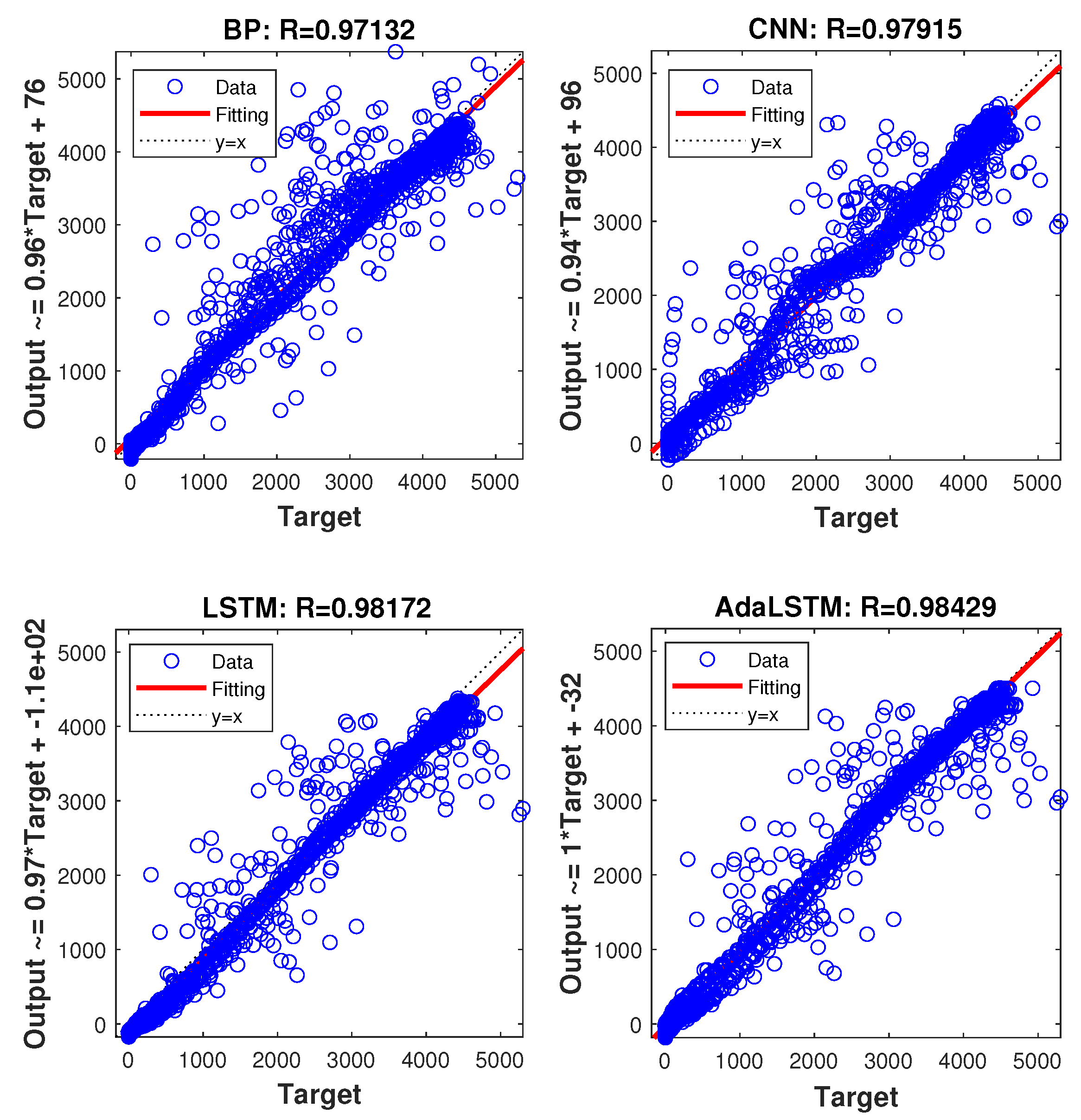
Table 3 shows comparison results of three performance metrics (Case A, average results of five independent runs). It can be seen that the proposed AdaLSTM model outperforms other models in terms of prediction accuracy for all three prediction horizons. Taking the 30 min prediction as an example, RMSE and MAE of the AdaLSTM model can be reduced, respectively, by 4.15% and 2.40%, and R 2 can increase by 0.40% compared with the LSTM model. In addition, it is observed that the prediction accuracy decreases as the prediction horizon increases. Using the real power (“Target”) as the x-axis and the predicted power (“Output”) as the y-axis, Figure 4 shows the scatter plots of four comparison models (30 min prediction). R denotes the multiple correlation coefficient [45]. As shown in Figure 4, the curve of AdaLSTM fitting is closest to line y = x and the corresponding R is the largest, which indicates that the AdaLSTM model has the highest prediction accuracy. Figure 5 shows the radar plot of performance metrics for comparison models (Case A, 30 min prediction). It is also seen that the AdaLSTM model is the best in terms of prediction accuracy.
For Case B, the same five models also perform the prediction tasks and their results are listed in Table 4 (average results of five independent runs). It is seen that the AdaLSTM model still has the highest accuracy under different prediction horizons. Compared with the basic LSTM model (30 min prediction), the RMSE and MAE of AdaLSTM are reduced, respectively, by 2.02% and 14.55%, and R 2 increases by 0.15%. Note that in Case B, the unit of PV solar power is kW instead of W in Case A. The results of the two cases demonstrate that the AdaLSTM prediction model has good accuracy and robustness for different PV solar power generation scales.

3.3. Validation of iPSO Based Data Clustering

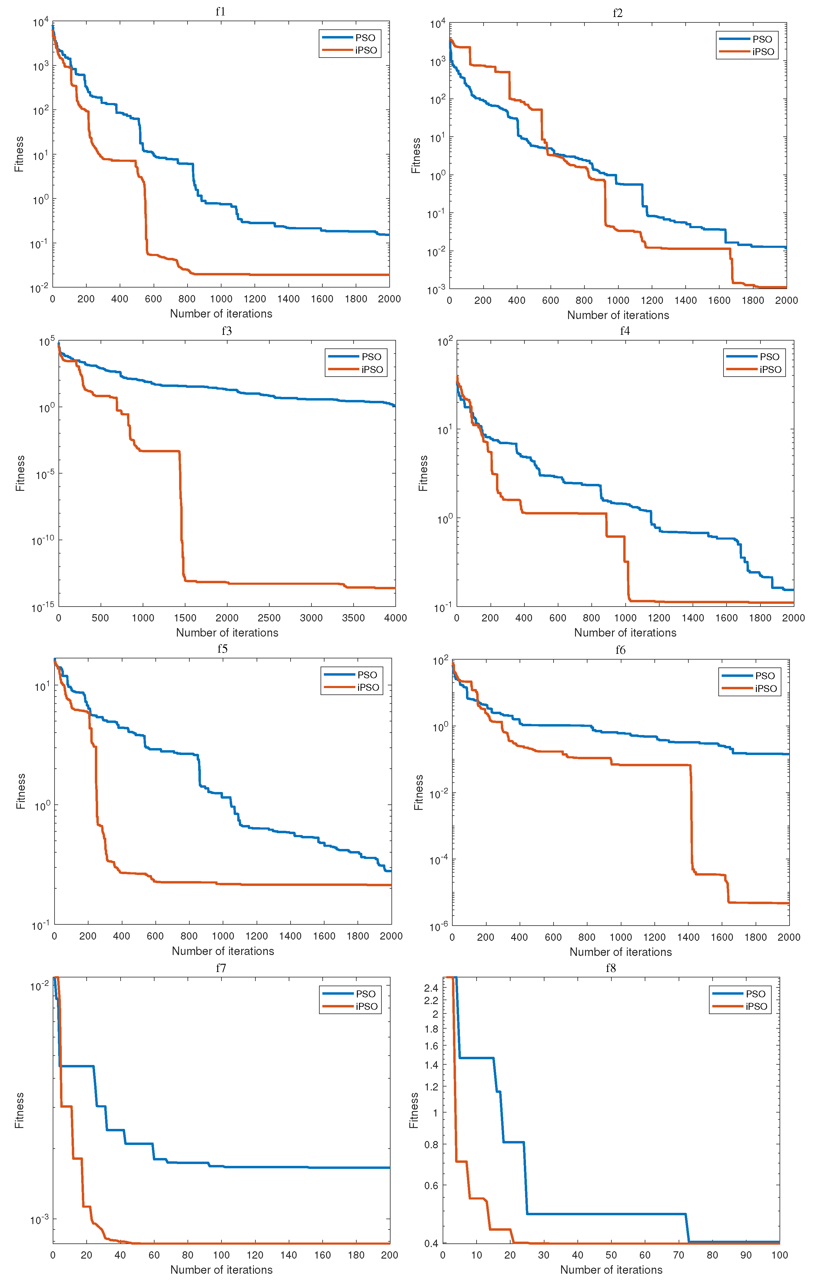
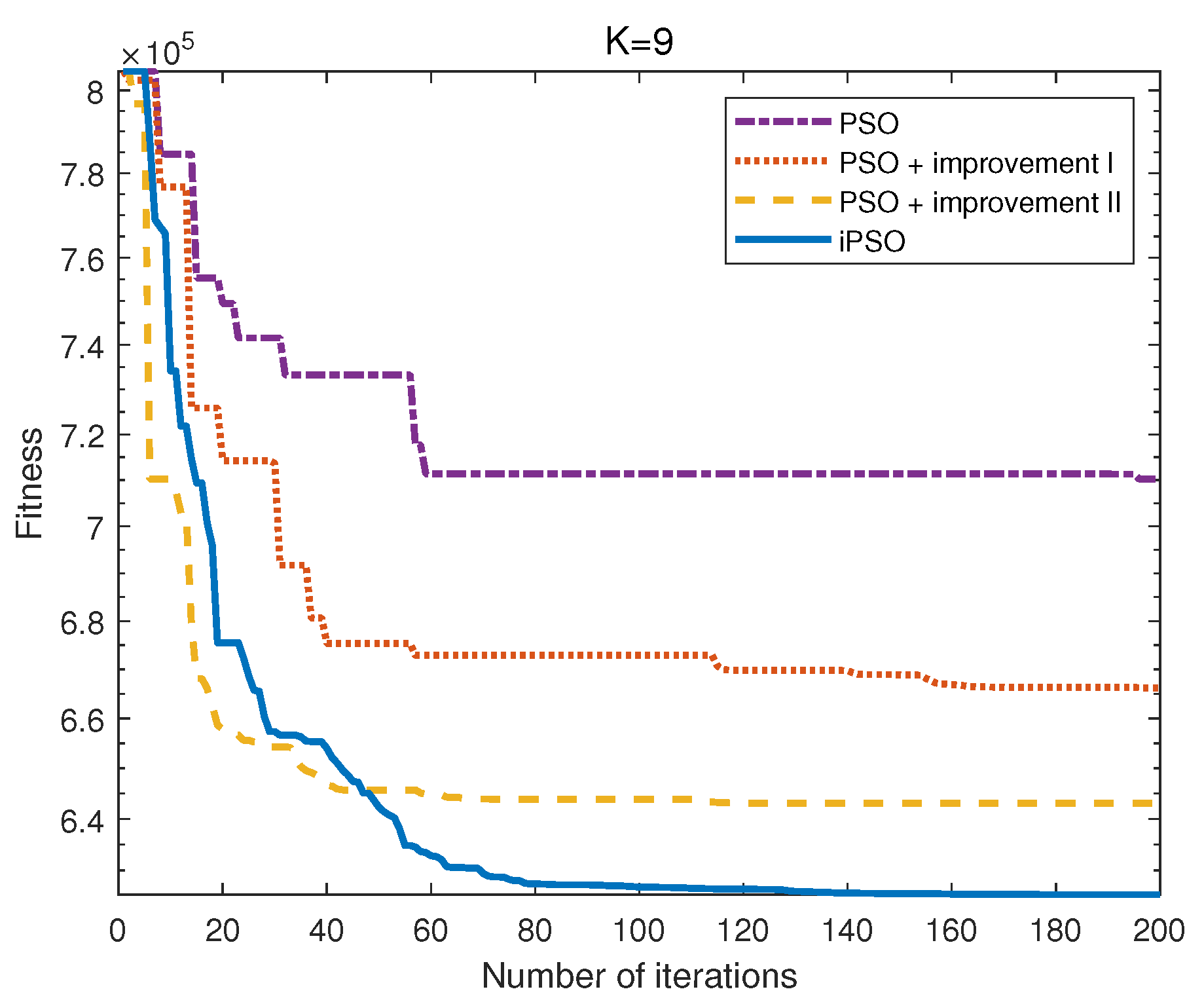
The performance of the iPSO algorithm is first verified using eight benchmark functions (see Table A1 in Appendix A for function details). The main parameters of iPSO are given in Table 5. Parameters ω max and c 1 are referred to in literature [46]. Other parameters such as swarm size and M are determined through trial and error. Comparison results of the convergence graphs between the PSO and iPSO algorithms are shown in Figure 6. The results demonstrate that, for each benchmark function, iPSO is superior to the basic PSO in terms of accuracy. Considering the convergence speed, the iPSO also outperforms the basic PSO for most benchmark functions (two algorithms have similar convergence speeds for f2 and f6). The designed iPSO algorithm is then used to search the optimal clustering centroids for Case A, and the convergence comparison with other algorithms is shown in Figure 7. It can be seen that for cluster centroid searching, the iPSO has the best accuracy with fast convergence speed.
Taking Case A as an example, the global irradiance and PV solar power are selected as the clustering features. The number of clusters K is set from 2 to 10. STDI is used to determine the K value, as shown in Table 6. It is seen that K = 9 corresponds to the largest STDI value. Moreover, after the iPSO-based data clustering with K = 9, the corresponding model (30 min prediction) has the highest prediction accuracy.

3.4. Influence of Clustering on Prediction Accuracy

In this section, the influence of iPSO-based clustering on PV solar power prediction is discussed. Prediction results without clustering, with K-means clustering and with iPSO based clustering, are compared using both Case A and Case B. At the same time, the 30-min data computation time of Case A is chosen to perform a balance analysis between computational burden and computational accuracy. Note that the AdaLSTM prediction model is adopted for each data cluster or for the situation of no clustering.
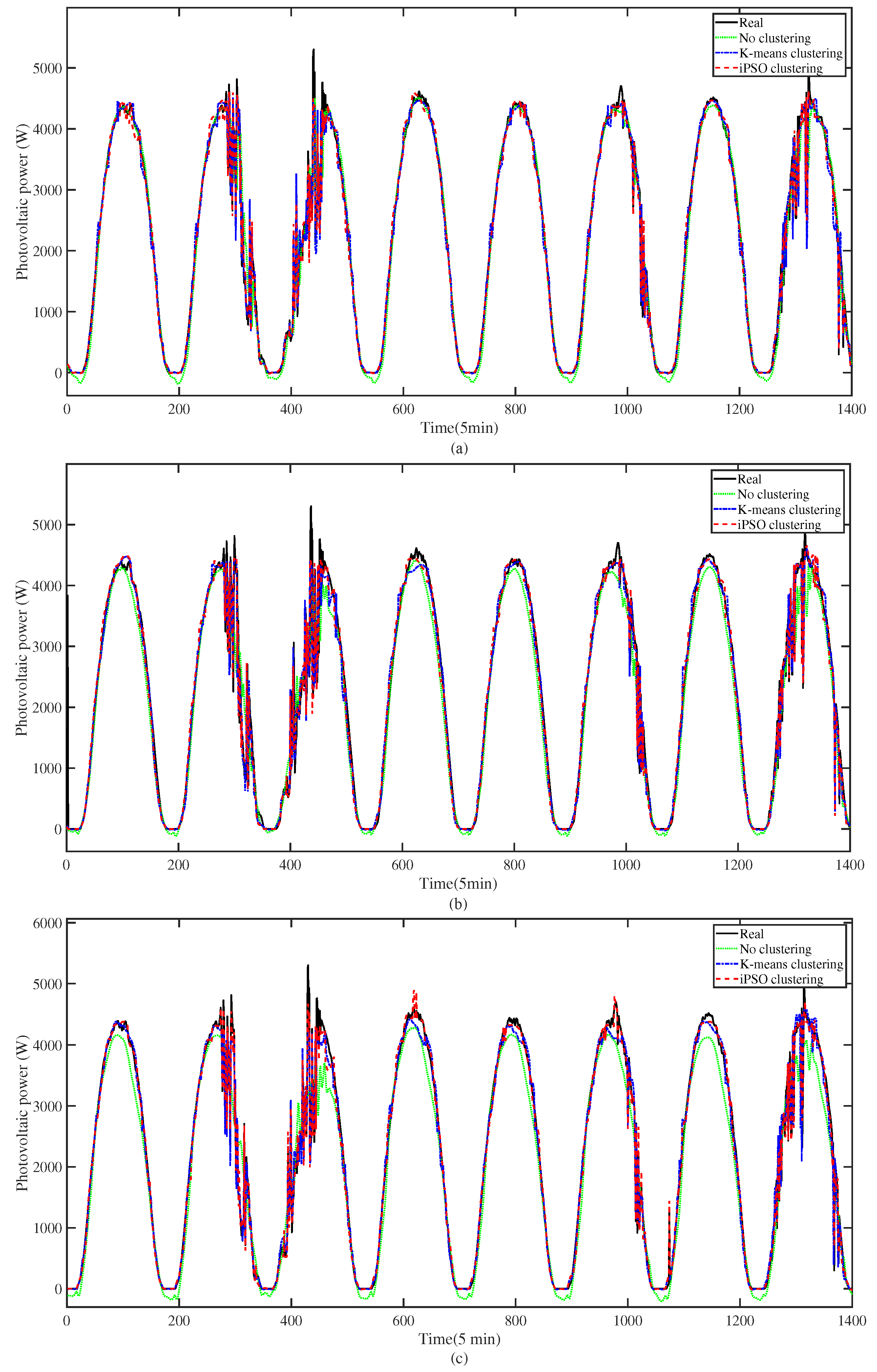
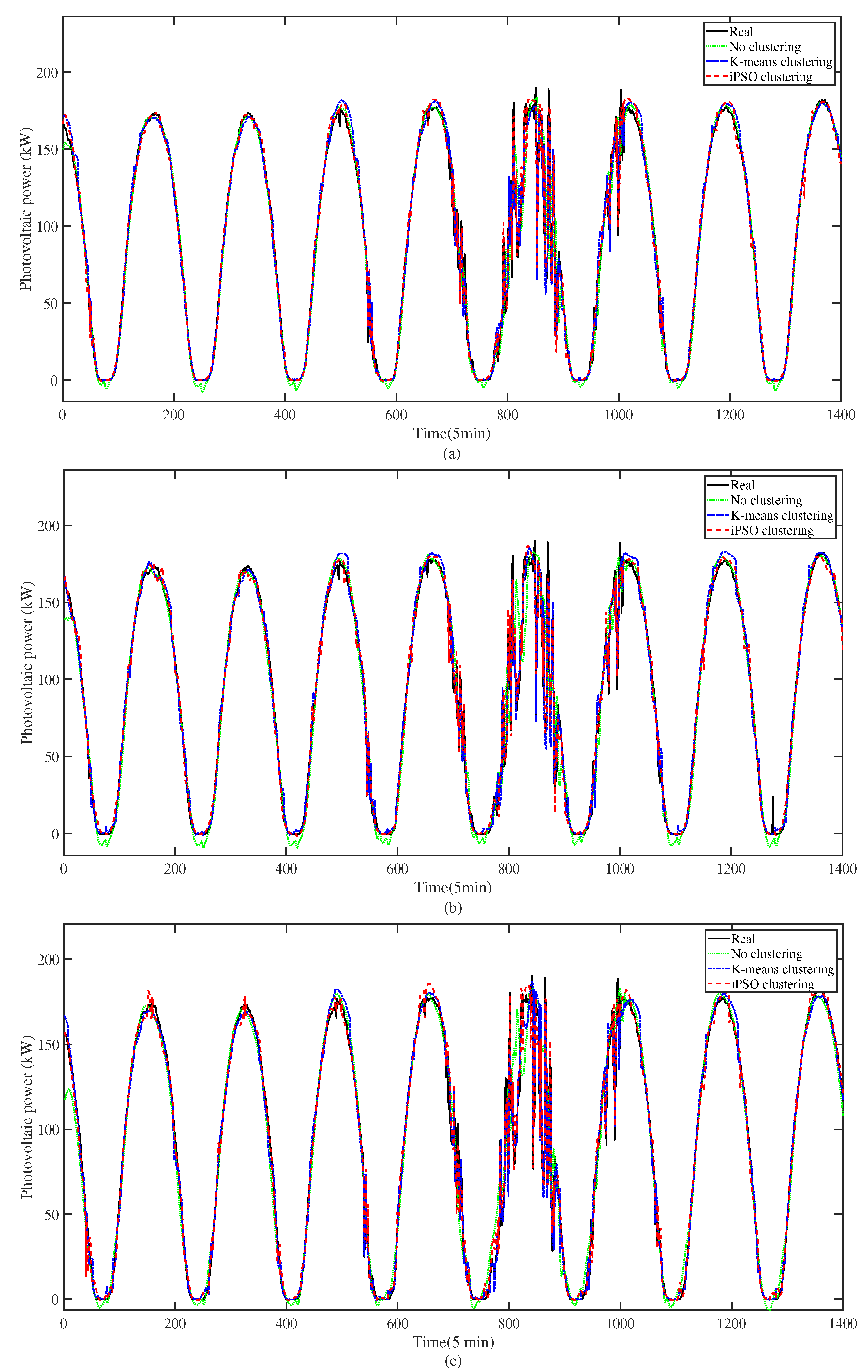
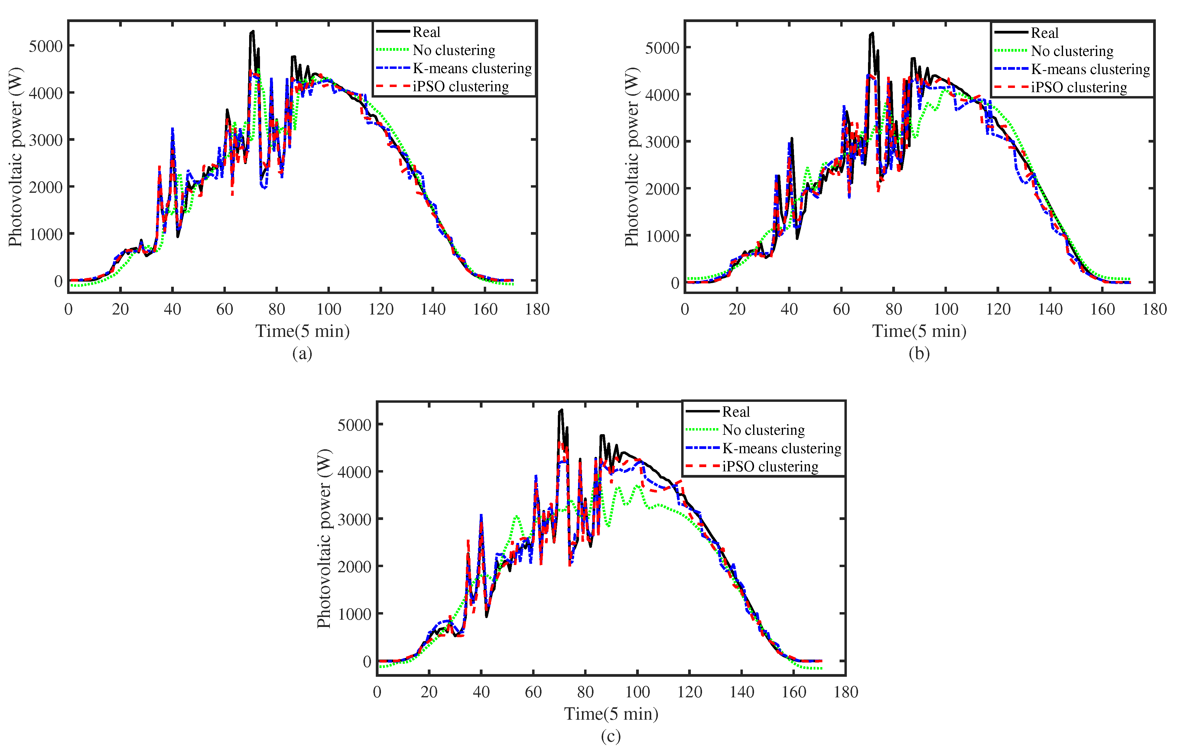
For Case A and Case B, performance metrics for different clustering methods are compared in Table 7 and Table 8, respectively (average results of five independent runs). It is seen that, for all three prediction horizons, the proposed iPSO-based clustering outperforms others in terms of prediction accuracy. Compared with the commonly used K-means clustering, RMSE and MAE of the prediction model with iPSO-based clustering are reduced, respectively, by 10.75% and 9.90%, and R 2 increases by 0.14% (Case A, 30 min prediction). RMSE and MAE are reduced, respectively, by 6.69% and 7.89%, and R 2 increases by 0.09% (Case B, 30 min prediction). Prediction curves based on all data in the testing set are compared in Figure 8 (Case A) and Figure 9 (Case B). The curve using measured values is marked as “Real”. It is known that, no matter which case is used, no matter which prediction horizon is addressed, iPSO-based clustering can bring significant improvement in prediction accuracy compared with K-means clustering and no clustering. Moreover, for easier observation of the differences between different clustering methods, Figure 10 and Figure 11 are provided to show just one-day prediction curves for Case A and Case B, respectively. It can be clearly seen that the prediction curve with iPSO-based clustering can track the real curve more accurately.
For the computational burden issue, time consumption for different models is shown in Table 9. It is clearly seen that, due to the data clustering, the training time of the proposed model is shorter than that of the AdaLSTM. Since model training could be conducted offline, the training time of 105.70 s is acceptable in real applications. In addition, the 10.74 s prediction time is also acceptable for 10, 30 or 60 min real-time prediction. These results further demonstrate the effectiveness and applicability of the proposed hybrid prediction model.

4. Discussion

According to the two case studies for multiple prediction horizons, the performance of the proposed PV solar power prediction model is investigated. A brief discussion on the effects of iPSO-based data clustering and AdaLSTM is provided as below.
The proposed iPSO includes two improvements: (1) Particles learn from only the best position; (2) The inertia weight is dynamically adjusted according to the individual fitness. iPSO is utilized to optimize the clustering centroids, which provides a better understanding of the internal patterns and characteristics of the PV dataset. From the results, it is seen that iPSO is generally superior to basic PSO in terms of accuracy and convergence speed. See Figure 6 for benchmark function comparison and Figure 7 for optimal clustering centroid searching. Note that the STDI is used to determine the number of data clusters. On the other hand, three basic LSTM networks are integrated in a serial manner through the AdaBoost algorithm to construct the AdaLSTM model. Prediction results show that AdaLSTM enhances the prediction accuracy in both cases. Compared with the basic LSTM, the RMSEs of AdaLSTM for 10 min, 30 min, and 60 min predictions are reduced, respectively, by 8.17%, 4.15%, and 5.14% (Case A) or 2.03%, 2.01%, and 2.95% (Case B).
By combining iPSO-based clustering and AdaBoost (see Section 2.3 for detailed process), prediction accuracy could be further improved. Compared with K-means clustering, the RMSEs of iPSO clustering for 10 min, 30 min, and 60 min predictions are reduced, respectively, by 6.36%, 10.75%, and 5.18% (Case A) or 10.69%, 6.69%, and 10.39% (Case B). Overall, the RMSE of the proposed hybrid model is reduced, respectively, by 75.22%, 73.80%, 67.60%, 66.30%, 64.85%, and 10.75% compared with persistence, BPNN, CNN, LSTM, AdaLSTM without clustering and AdaLSTM with K-means clustering (Case A, 30 min prediction). For the computational burden (see Table 9), it is known that the training time of the proposed model (105.70 s) is shorter than that of the AdaLSTM (223.68 s), but longer than that of the basic LSTM (70.40 s). Considering the model training could be conducted offline, about 2 min of training time is acceptable in real applications. Moreover, the prediction time of 10.74 s is also acceptable for 10, 30, or 60 min PV solar power prediction.

5. Conclusions

In order to discover the potential distribution patterns of PV data and enhance the accuracy and reliability of solar power prediction, a hybrid prediction model is proposed in this paper based on iPSO-based clustering and the AdaLSTM network. For data clustering, the clustering centroids are optimized by the iPSO algorithm. For each data cluster, the AdaBoost algorithm and multiple basic LSTM networks are combined together to form the AdaLSTM model for model training. Final prediction results are obtained using the KNN method and the corresponding trained AdaLSTM model. Datasets from two PV stations in Australia are adopted for case studies. The results show that the AdaLSTM model outperforms other existing prediction models such as persistence, BPNN, CNN and LSTM. The RMSE and MAE can be reduced, respectively, by 4.15% and 2.40% compared with the best comparison model (Case A, 30 min prediction). Further, the analysis of iPSO in terms of accuracy and convergence speed and the prediction accuracy comparison between no clustering, K-means clustering, and iPSO-based clustering are performed to verify the superiority of the proposed hybrid model. Compared with the commonly used K-means clustering, the RMSE and MAE of the prediction model with iPSO-based clustering are reduced, respectively, by 10.75% and 9.90% (Case A, 30 min prediction). It is worth noting that during the data clustering process, the sum of the Euclidean distances of all data to the nearest centroid is chosen as the fitness function for iPSO, which indicates that unsupervised clustering is performed in this paper. In future research, feature selection of the prediction model will be studied, and the training error will be used to design the fitness function of iPSO to achieve supervised data clustering.

Author Contributions

Conceptualization, W.X.; methodology, W.X.; software, J.L.; validation, K.L.; formal analysis, J.L.; data curation, J.L.; writing—original draft preparation, J.L.; writing—review and editing, W.X.; supervision, K.L. and W.X.; funding acquisition, K.L. All authors have read and agreed to the published version of the manuscript.

Funding

This research was funded by National Natural Science Foundation of China under Grant number 61873114; Six Talent Peaks Project in Jiangsu Province under Grant number JZ-053 and Key Research and Development Program in Zhenjiang City under Grant number SH2023108.

Data Availability Statement

The data that support the findings of this study are available from the corresponding author upon reasonable request.

Conflicts of Interest

The authors declare no conflicts of interest.

Nomenclature

AdaBoostadaptive boosting
AdaLSTMadaptive boosting LSTM
ANNartificial neural network
ARMAautoregressive moving average model
BPNNback propagation neural network
CBclustering-based
CHOAchimp optimization algorithm
CNNconvolutional neural networks
DTCWTdual tree complex wavelet transforms
EEMDensemble empirical mode decomposition
ELMextreme learning machine
iPSOimproved particle swarm optimization
KNNk-nearest neighbor
KSVDk-singular value decomposition
LSSVMleast squares support vector machine
LSSVRleast square support vector regression
LSTMlong short-term memory
MAEmean absolute error
MHFMmultiscale hybrid forecast model
MLPmultilayer perceptron
MLPNNmultilayer perceptron neural network
MTLBOmodified teaching learning based optimization
NARnonlinear autoregressive
NNEneural network ensemble
PCAprincipal components analysis
PSOparticle swarm optimization
PVphotovoltaic
Rmultiple correlation coefficient
R 2 coefficient of determination
RVFLrandom vector functional link
RMSEroot mean square error
RNNrecurrent neural network
RVFLNrandom vector functional link network
SCADAsupervisory control and data acquisition
STDIstandard deviation based index
SVMsupport vector machine
VMDvariational mode decomposition
WRFweather research and forecasting
WTwavelet transform
p b e s t i best position of particle i
g b e s t position of the best particle
P c learning probability of particle i
P s population size
mrefresh pointer
ω inertia weight
ω min minimum of inertia weight
ω max maximum of inertia weight
f min minimum fitness of all particles
f a v g average fitness of all particles
Knumber of clusters
T h prediction horizon

Appendix A

Table A1. Benchmark functions.
FunctionDomain
f 1 = i = 1 30 x i 2 [−100, 100]
f 2 = i = 1 30 i x i 2 [−10, 10]
f 3 = i = 1 30 ( j = 1 i x j ) 2 [−100, 100]
f 4 = max { | x i | , 1 i 30 } [−100, 100]
f 5 = 20 exp ( 0.2 1 30 i = 1 30 x i 2 ) exp ( 1 30 i = 1 30 cos ( 2 π x i ) ) + 20 + e [−32, 32]
f 6 = 1 4000 i = 1 30 x i 2 i = 1 30 cos x i i + 1 [−600, 600]
f 7 = i = 1 11 [ a i x 1 ( b i 2 + b i x 2 ) b i 2 + b 1 x 3 + x 4 ] 2
a i = [0.1957, 0.1947, 0.1735, 0.16, 0.0844, 0.0627, 0.0456, 0.0342, 0.0323, 0.0235, 0.0246]
b i = 1 [ 0.25 , 0.5 , 1 , 2 , 4 , 6 , 8 , 10 , 12 , 14 , 16 ] [−5, 5]
f 8 = ( x 2 5.1 4 π 2 x 1 2 + 5 π x 1 6 ) 2 + 10 ( 1 1 8 π ) cos x 1 + 10 x 1 ∈ [−5, 10] x 2 ∈ [0, 15]

References

  1. Voyant, C.; Notton, G.; Kalogirou, S.; Nivet, M.-L.; Paoli, C.; Motte, F.; Fouilloy, A. Machine learning methods for solar radiation forecasting: A review. Renew. Energy 2017, 105, 569–582. [Google Scholar] [CrossRef]
  2. Tawn, R.; Browell, J. A review of very short-term wind and solar power forecasting. Renew. Sustain. Energy Rev. 2022, 153, 111758. [Google Scholar] [CrossRef]
  3. Huang, X.; Zhang, C.; Li, Q.; Tai, Y.; Shi, J. A Comparison of Hour-Ahead Solar Irradiance Forecasting Models Based on LSTM Network. Math. Probl. Eng. 2020, 2020, 4251517. [Google Scholar] [CrossRef]
  4. Cao, J.; Cao, S. Study of forecasting solar irradiance using neural networks with preprocessing sample data by wavelet analysis. Energy 2006, 31, 3435–3445. [Google Scholar] [CrossRef]
  5. Voyant, C.; Muselli, M.; Paoli, C.; Nivet, M.-L. Numerical Weather Prediction (NWP) and hybrid ARMA/ANN model to predict global radiation. Energy 2012, 39, 341–355. [Google Scholar] [CrossRef]
  6. Monjoly, S.; André, M.; Calif, R.; Soubdhan, T. Forecast horizon and solar variability influences on the performances of multiscale hybrid forecast model. Energies 2019, 12, 2264. [Google Scholar] [CrossRef]
  7. Eseye, A.T.; Zhang, J.; Zheng, D. Short-term photovoltaic solar power forecasting using a hybrid Wavelet-PSO-SVM model based on SCADA and Meteorological information. Renew. Energy 2018, 118, 357–367. [Google Scholar] [CrossRef]
  8. Olatomiwa, L.; Mekhilef, S.; Shamshirband, S. Global Solar Radiation Forecasting Based on SVM-Wavelet Transform Algorithm. Int. J. Intell. Syst. Appl. (IJISA) 2016, 8, 19–26. [Google Scholar] [CrossRef]
  9. Sahu, R.K.; Shaw, B.; Nayak, J.R. Short/medium term solar power forecasting of Chhattisgarh state of India using modified TLBO optimized ELM. Eng. Sci. Technol. Int. J. 2021, 24, 1180–1200. [Google Scholar] [CrossRef]
  10. Wang, S.; Wang, Y.; Liu, Y.; Zhang, N. Hourly solar radiation forecasting based on EMD and ELM neural network. Electr. Power Autom. Equip. 2014, 34, 7–12. [Google Scholar]
  11. Zayed, M.E.; Zhao, J.; Li, W.; Elsheikh, A.H.; Abd Elaziz, M.; Yousri, D.; Zhong, S.; Mingxi, Z. Predicting the performance of solar dish Stirling power plant using a hybrid random vector functional link/chimp optimization model. Sol. Energy 2021, 222, 1–17. [Google Scholar] [CrossRef]
  12. Zayed, M.E.; Aboelmaaref, M.M.; Chazy, M. Design of solar air conditioning system integrated with photovoltaic panels and thermoelectric coolers: Experimental analysis and machine learning modeling by random vector functional link coupled with white whale optimization. Therm. Sci. Eng. Prog. 2023, 44, 102051. [Google Scholar] [CrossRef]
  13. De Araujo, J.M.S. Combination of WRF model and LSTM network for solar radiation forecasting—Timor leste case study. Comput. Water Energy Environ. Eng. 2020, 9, 108–144. [Google Scholar] [CrossRef]
  14. Hong, Y.-Y.; Martinez, J.J.F.; Fajardo, A.C. Day-ahead solar irradiation forecasting utilizing gramian angular field and convolutional long short-term memory. IEEE Access 2020, 8, 18741–18753. [Google Scholar] [CrossRef]
  15. Ren, Y.; Wang, J.; Yang, C.; Xiao, C.; Li, S. Wind and Solar Integrated Power Prediction Method Research Based on DT-CWT and LSTM. J. Phys. Conf. Ser. 2021, 1745, 012008. [Google Scholar] [CrossRef]
  16. Wang, J.; Li, J. Short-term Photovoltaic Power Forecasting Using the Combined KSVD and LSTM Method. In Proceedings of the 2022 International Conference on Machine Learning, Cloud Computing and Intelligent Mining (MLCCIM 2022), Xiamen, China, 5–7 August 2022; pp. 134–138. [Google Scholar]
  17. Elizabeth Michael, N.; Mishra, M.; Hasan, S.; Al-Durra, A. Short-term solar power predicting model based on multi-step CNN stacked LSTM technique. Energies 2022, 15, 2150. [Google Scholar] [CrossRef]
  18. Wang, K.; Qi, X.; Liu, H. Photovoltaic power forecasting based LSTM-Convolutional Network. Energy 2019, 189, 116225. [Google Scholar] [CrossRef]
  19. Zhang, C.; Yan, Z.; Ma, C.; Xu, X. Prediction of direct normal irradiation based on CNN-LSTM model. In Proceedings of the 2020 5th International Conference on Multimedia Systems and Signal Processing, Chengdu, China, 8–10 May 2020; pp. 74–80. [Google Scholar]
  20. Kumar, J.; Goomer, R.; Singh, A.K. Long short term memory recurrent neural network (LSTM-RNN) based workload forecasting model for cloud datacenters. Procedia Comput. Sci. 2018, 125, 676–682. [Google Scholar] [CrossRef]
  21. Chaouachi, A.; Kamel, R.M.; Nagasaka, K. Neural network ensemble-based solar power generation short-term forecasting. J. Adv. Comput. Intell. Intell. Inform. 2010, 14, 69–75. [Google Scholar] [CrossRef]
  22. Liu, J.; Huang, X.; Li, Q.; Chen, Z.; Liu, G.; Tai, Y. Hourly stepwise forecasting for solar irradiance using integrated hybrid models CNN-LSTM-MLP combined with error correction and VMD. Energy Convers. Manag. 2023, 280, 116804. [Google Scholar] [CrossRef]
  23. Zhou, Y.; Xue, W.; Liu, J.; Li, K. Photovoltaic power prediction based on SVMD-PCA-EL model. In Proceedings of the 2022 41st Chinese Control Conference (CCC), Hefei, China, 25–27 July 2022; pp. 5621–5626. [Google Scholar]
  24. Benmouiza, K.; Cheknane, A. Forecasting hourly global solar radiation using hybrid k-means and nonlinear autoregressive neural network models. Energy Convers. Manag. 2013, 75, 561–569. [Google Scholar] [CrossRef]
  25. Azimi, R.; Ghayekhloo, M.; Ghofrani, M. A hybrid method based on a new clustering technique and multilayer perceptron neural networks for hourly solar radiation forecasting. Energy Convers. Manag. 2016, 118, 331–344. [Google Scholar] [CrossRef]
  26. Malakar, S.; Goswami, S.; Ganguli, B.; Chakrabarti, A.; Roy, S.S.; Boopathi, K.; Rangaraj, A.G. Deep-learning-based adaptive model for solar forecasting using clustering. Energies 2022, 15, 3568. [Google Scholar] [CrossRef]
  27. Sun, S.; Wang, S.; Zhang, G.; Zheng, J. A decomposition-clustering-ensemble learning approach for solar radiation forecasting. Sol. Energy 2018, 163, 189–199. [Google Scholar] [CrossRef]
  28. Kennedy, J.; Eberhart, R. Particle swarm optimization. Int. Conf. Neural Netw. 1995, 4, 1942–1948. [Google Scholar]
  29. Bai, Q. Analysis of particle swarm optimization algorithm. Comput. Inf. Sci. 2010, 3, 180. [Google Scholar] [CrossRef]
  30. Cai, L.; Hou, Y.; Zhao, Y.; Wang, J. Application research and improvement of particle swarm optimization algorithm. In Proceedings of the 2020 IEEE International Conference on Power, Intelligent Computing and Systems (ICPICS), Shenyang, China, 28–30 July 2020; pp. 238–241. [Google Scholar]
  31. Liang, J.J.; Qin, A.K.; Suganthan, P.N.; Baskar, S. Comprehensive learning particle swarm optimizer for global optimization of multimodal functions. IEEE Trans. Evol. Comput. 2006, 10, 281–295. [Google Scholar] [CrossRef]
  32. El-Zonkoly, A.; Saad, M.; Khalil, R. New algorithm based on CLPSO for controlled islanding of distribution systems. Int. J. Electr. Power Energy Syst. 2013, 45, 391–403. [Google Scholar] [CrossRef]
  33. Chen, X.; Wang, B.; Yu, M.; Jin, J.; Xu, W. The interpolation of missing wind speed data based on optimized LSSVM model. In Proceedings of the 2016 IEEE 8th International Power Electronics and Motion Control Conference (IPEMC-ECCE Asia), Hefei, China, 22–26 May 2016; pp. 1448–1451. [Google Scholar]
  34. Wang, W.; Cheng, J.; Gao, Y.; Yu, X. A scenario reduction method of PV output based on NBSO algorithm and STDI index. J. Phys. Conf. Ser. 2023, 2496, 012005. [Google Scholar] [CrossRef]
  35. Yu, Y.; Si, X.; Hu, C.; Zhang, J. A review of recurrent neural networks: LSTM cells and network architectures. Neural Comput. 2019, 31, 1235–1270. [Google Scholar] [CrossRef]
  36. Bai, Y.; Xie, J.; Wang, D.; Zhang, W.; Li, C. A manufacturing quality prediction model based on AdaBoost-LSTM with rough knowledge. Comput. Ind. Eng. 2021, 155, 107227. [Google Scholar] [CrossRef]
  37. Zhang, M.-L.; Zhou, Z.-H. ML-KNN: A lazy learning approach to multi-label learning. Pattern Recognit. 2007, 40, 7. [Google Scholar] [CrossRef]
  38. DKA Solar Centre. Available online: https://dkasolarcentre.com.au/download?location=alice-springs (accessed on 20 February 2024).
  39. DKA Solar Centre. Available online: https://dkasolarcentre.com.au/download?location=yulara (accessed on 20 February 2024).
  40. Pedro, H.T.C.; Coimbra, C.F.M. Assessment of forecasting techniques for solar power production with no exogenous inputs. Sol. Energy 2012, 86, 2017–2028. [Google Scholar] [CrossRef]
  41. Wang, Z.; Wang, F.; Su, S. Solar irradiance short-term prediction model based on BP neural network. Energy Procedia 2011, 12, 488–494. [Google Scholar] [CrossRef]
  42. Agga, A.; Abbou, A.; Labbadi, M.; El Houm, Y.; Ali, I.H.O. CNN-LSTM: An efficient hybrid deep learning architecture for predicting short-term photovoltaic power production. Electr. Power Syst. Res. 2022, 208, 107908. [Google Scholar] [CrossRef]
  43. Abdel-Nasser, M.; Mahmoud, K. Accurate photovoltaic power forecasting models using deep LSTM-RNN. Neural Comput. Appl. 2019, 31, 2727–2740. [Google Scholar] [CrossRef]
  44. Wei, B.; Li, K.; Zhou, S.; Xue, W.; Tan, G. An instance based multi-source transfer learning strategy for building’s short-term electricity loads prediction under sparse data scenarios. J. Build. Eng. 2024, 85, 108713. [Google Scholar] [CrossRef]
  45. Asuero, A.G.; Sayago, A.; González, A.G. The correlation coefficient: An overview. Crit. Rev. Anal. Chem. 2006, 36, 41–59. [Google Scholar] [CrossRef]
  46. Lin, A.; Sun, W.; Yu, H.; Wu, G.; Tang, H. Adaptive comprehensive learning particle swarm optimization with cooperative archive. Appl. Soft Comput. 2019, 77, 533–546. [Google Scholar] [CrossRef]
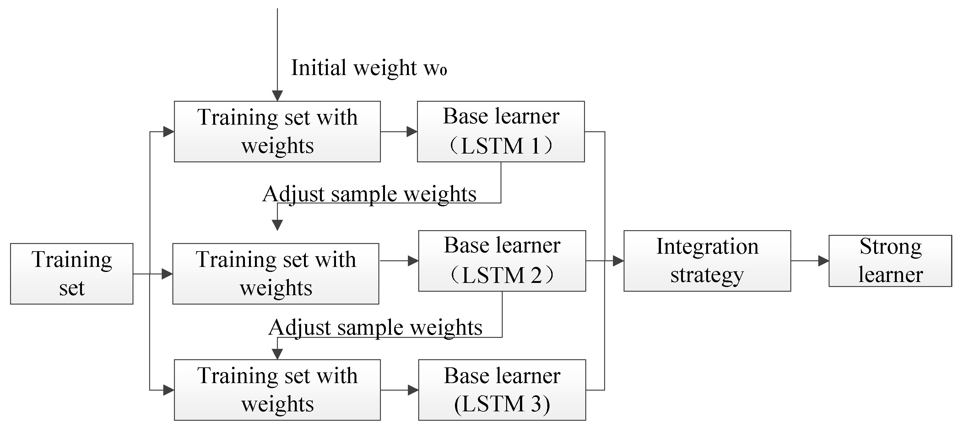
Figure 2. Structure of AdaLSTM model.
Energies 17 01624 g002
Figure 3. Overall prediction framework.
Energies 17 01624 g003
Figure 4. Prediction output scatter plots of different models (Case A, no clustering).
Energies 17 01624 g004
Figure 5. Radar plot of performance metrics (Case A, no clustering): (a) RMSE, (b) MAE, (c) R 2 .
Energies 17 01624 g005
Figure 6. Convergence graphs of eight benchmark functions using PSO and iPSO.
Energies 17 01624 g006
Figure 7. Convergence graph of clustering centroid optimization using different algorithms (Case A).
Energies 17 01624 g007
Figure 8. Prediction curves (Case A, 8 February 2020–16 February 2020): (a) 10 min prediction, (b) 30 min prediction, (c) 60 min prediction.
Energies 17 01624 g008
Figure 9. Prediction curves (Case B, 15 February 2020–23 February 2020): (a) 10 min prediction, (b) 30 min prediction, (c) 60 min prediction.
Energies 17 01624 g009
Figure 10. Prediction curves (Case A, from 5:30 to 20:00 on 11 February 2020): (a) 10 min prediction, (b) 30 min prediction, (c) 60 min prediction.
Energies 17 01624 g010
Figure 11. Prediction curves (Case B, from 5:30 to 20:00 on 21 February 2020): (a) 10 min prediction, (b) 30 min prediction, (c) 60 min prediction.
Energies 17 01624 g011
Table 1. Literature review on PV solar energy prediction.
RefLocationMethodDataset Covering TimePerformance MetricsCharacteristic
[3]ColoradoLSTM-MLP1 January 2012 to 31 December 2016RMSE (62.1618 W/m2)The role of lag time was significant when the input variables of the LSTM model were small.
[5]Mediterranean areaANNOctober 2002 to December 2008nRMSE (14.9%)A hybrid approach that utilized a coupled artificial neural network (ANN) and autoregressive moving average (ARMA) predictors could substantially decrease prediction errors.
[6]Guadeloupe islandMHFM modelJanuary 2012 to December 2012nRMSE (4.43–10.24%)Four types of typical days were identified and datasets were established for each.
[7]BeijingHybrid WT-PSO-SVMone year with a time step of 10 minMAPE (4.22%)The PSO was used to optimize the parameters of the SVM in order to achieve a higher forecasting accuracy.
[9]ChhattisgarhMTLBO-ELMFebruary 2019 to December 2019MAPE (8.2091%)ELM models based on MTLBO optimization outperformed ELM, ELM (randomly fixed weights and biases), and ANN models based on different optimizations.
[11]ArizonaREVL-CHOAMarch 2010 to June 2011RMSE (0.00047, 0.05995)The RFVL-CHOA method was found to be superior and more effective than other optimization models studied for performance prediction.
[12]SohagRVFLN-WWONA R 2 ( 1.00 ; 0.9151 ) The experimental results uniquely fitted with the predicted results of the proposed artificial intelligence model.
[13]DiliWRF-LSTMJanuary to December 2014nRMSE (16.18%)The combination of the WRF and LSTM methods had better performance and could be applied to simulate other locally relevant weather variables.
[14]TaiwanCNN-LSTN5 January 2017 to 4 January 2018RMSE (0.0472)The network allowed for time series forecasting using a feature-rich approach, resulting in competitive forecasting performance even with small datasets.
[16]Yulara soalr systemKSVD-LSTM7 March to 7 June 2021RMSE (0.3682)The combined method of KSVD and LSTM achieved highly accurate prediction results.
[17]Abu DhabiCNN-LSTMJuly 2019RMSE (0.36)The model predicts both solar irradiance and POA more accurately than what has been reported in the literature.
[18]Alice SpringsLSTM-Convolutional Networkhalf yearRMSE (0.621)The proposed hybrid model outperformed the convolutional LSTM network and had a better prediction effect than the single prediction model.
[20]AlbertaLSTM-RNNseven monthsMSE (0.00317)The hybrid model had higher accuracy.
[21]TUATNNE2007 to 2008MAPE (3.6387)Compared with traditional networks, neural network ensembles exhibited the highest level of prediction accuracy.
[22]FolsomCNN-LSTM-MLP1 January 2014 to 31 December 2016RMSE (12.53 W/m2)The model was more accurate and robust than many traditional alternative methods.
[25]AmesKmeans-mlpnn08/25–31/2013RMSE (32.01 W/m2)The comparison with the benchmark solar radiation forecast model indicated that the model had superior forecasting capabilities.
[24]AlgeriaKmeans-NARJanuary 1994 to December 1996nRMSE (0.1985)The obtained experimental results showed that the clustering of the input space was an important task to interpret the behavior of the series.
[26]BegamganjCB-LSTM2013nRMSE (19.74)The performance was improved compared with a single site-specific model.
[27]BeijingEEMD-LSSVR-K-LSSVR1 January 2009 to 30 June 2017nRMSE (2.96%)The DCE learning method showed promise for predicting solar radiation, with high levels of horizontal and directional accuracy, as well as robustness.
Table 2. Main parameters of AdaLSTM.
ParameterSetting
MaxEpochs100
Maximum number of iterations100
Number of hidden neurons200
Initial learn rate0.004
Learn rate drop period90
Learn rate drop factor0.2
Table 3. Performance metrics of different models (Case A, no clustering).
Prediction HorizonModelRMSE (W)MAE (W) R 2
Persistence311.89159.800.9655
BP381.46216.800.9477
10 minCNN328.11186.040.9616
LSTM324.06191.530.9626
AdaLSTM297.58155.790.9685
Persistence489.55352.640.9150
BP463.10308.260.9236
30 minCNN374.39253.010.9498
LSTM360.05240.330.9538
AdaLSTM345.12234.570.9576
Persistence834.88654.250.7516
BP698.60477.880.8261
60 minCNN411.13281.150.9396
LSTM384.51271.860.9471
AdaLSTM364.76246.500.9526
Table 4. Performance metrics of different models (Case B, no clustering).
Prediction HorizonModelRMSE (kW)MAE (kW) R 2
Persistence15.297.430.9462
BP12.656.280.9637
10 minCNN12.376.650.9652
LSTM12.085.480.9669
AdaLSTM11.845.400.9684
Persistence22.5015.130.8835
BP15.408.860.9461
30 minCNN14.128.140.9546
LSTM12.397.010.9651
AdaLSTM12.145.990.9665
Persistence32.8225.550.7562
BP20.9714.170.8990
60 minCNN15.728.890.9437
LSTM13.637.760.9577
AdaLSTM13.247.610.9601
Table 5. Main parameter of iPSO.
ParameterSetting
Swarm size50
ω max 0.89
ω min 0.7
M10
c 1 1.5
Table 6. Comparison of indexes for different K (Case A).
KSTDI ValueRMSE (W)MAE (W) R 2
210277.04159.060.9727
325258.84154.010.9761
481199.53121.310.9858
5229201.37131.160.9856
6374160.43108.270.9901
7529169.44112.960.9898
8659189.64121.570.9911
91801126.0988.580.9943
101488135.9588.210.9934
Table 7. Performance metrics for different clustering methods (Case A).
Prediction HorizonClustering MethodRMSE (W)MAE (W) R 2
No clustering297.58155.790.9685
10 minK-means clustering125.0780.950.9944
iPSO based clustering117.1179.080.9951
No clustering345.12234.570.9576
30 minK-means clustering135.9491.200.9934
iPSO based clustering121.3282.170.9948
No clustering364.76246.500.9526
60 minK-means clustering134.8689.990.9935
iPSO based clustering127.8787.210.9941
Table 8. Performance metrics for different clustering methods (Case B).
Prediction HorizonClustering MethodRMSE (kW)MAE (kW) R 2
No clustering11.845.400.9684
10 minK-means clustering5.523.590.9930
iPSO based clustering4.933.290.9945
No clustering12.145.990.9665
30 minK-means clustering5.533.930.9930
iPSO based clustering5.163.620.9939
No clustering13.247.610.9601
60 minK-means clustering6.164.130.9913
iPSO based clustering5.523.820.9936
Table 9. Time consumption for different models (Case A, 30 min prediction).
ModelTraining Time (s)Prediction Time (s)
LSTM70.404.29
AdaLSTM223.6813.15
iPSO clustering + AdaLSTM105.7010.74
Disclaimer/Publisher’s Note: The statements, opinions and data contained in all publications are solely those of the individual author(s) and contributor(s) and not of MDPI and/or the editor(s). MDPI and/or the editor(s) disclaim responsibility for any injury to people or property resulting from any ideas, methods, instructions or products referred to in the content.