Generation and Transmission Expansion Planning Using a Nested Decomposition Algorithm

Abstract

This work presents an implementation of a Nested Decomposition Algorithm (NDA) applied to co-optimizing generation and transmission capacity expansion planning problems in power systems, including operational flexibility constraints. The proposed methodology has been gaining relevance in recent years, as it can efficiently solve large mixed-integer problems faster than the conventional extensive formulation (mixed-integer linear programming). Three case studies are conducted on two IEEE test power systems to evaluate the algorithm’s performance and cut configuration. The first case study compares the performance between the NDA and the extensive formulation. The second case study compares the performance of each cut type, analyzing differences in simulation times and algorithm convergence. The third case study proposes a set of cut patterns based on the prior outcomes, whose performance and convergence are tested. Based on the simulation results, conclusions are drawn about the capability and performance of the NDA applied to the capacity expansion planning problem. The study shows that obtaining results with reasonable convergence in less simulation time is possible using a particular pattern.

1. Introduction

Generation and transmission capacity expansion planning is a critical and complex challenge in the electricity industry, aiming to optimize long-term investment decisions in generation and transmission infrastructure to meet future electricity demand reliably, securely, and economically. As global energy systems transition towards more sustainable and resilient structures, the intricacies of planning are magnified by the integration of renewable energy sources, deregulated markets, and the imperative to reduce carbon emissions. The Generation and Transmission Capacity Expansion Planning (GTCEP) problem involves strategizing the optimal mix and timing of generation technologies and transmission expansion, over a multi-decade horizon, while minimizing total system costs, including both investment and operational expenses.

The Nested Decomposition Algorithm (NDA) presented in this work offers a robust model and methodology that significantly enhances the analytical capabilities available to power system planners and researchers. Our approach addresses the GTCEP problem by efficiently solving large mixed-integer problems, incorporating operational flexibility constraints that are crucial for accommodating the variability and uncertainty inherent in renewable energy resources and future demand projections. This model is not merely an academic exercise but is designed with practical application in mind. It is intended for use in everyday research and planning exercises, providing a valuable tool for verifying development plans and investment strategies in the energy sector. By improving the speed and accuracy of these complex decision-making processes, the NDA facilitates more informed, cost-effective, and forward-looking planning outcomes.

Targeted towards utilities, system operators, regulatory bodies, and policymakers, our methodology aims to support the strategic planning and policy formulation necessary for transitioning to more sustainable and resilient power systems. In doing so, it contributes to the broader goals of ensuring energy security, economic efficiency, and environmental sustainability in the face of evolving technological, market, and regulatory landscapes.

1.1. Technical Literature Review

Over the years, numerous planning models and optimization techniques have been developed to address the complexity and uncertainty associated with power systems. These models and procedures have evolved from traditional deterministic programming to stochastic programming [1] and from single-stage to multistage optimization frameworks [2]. Deterministic models assume that all the inputs and parameters are known with certainty, whereas stochastic models consider the uncertainty associated with load growth, fuel prices, and other factors [3].

Including binary power unit commitment (ON/OFF status) and operational constraints in planning models makes the GTCEP problem significantly complex. The interaction between three types of binary variables, generation investment decisions, transmission investment decisions and unit commitment decisions, implies a different behavior in terms of algorithm convergence. On the one hand, generation investments affect the unit commitment problem. On the other hand, the transmission investments react to new generation investments and vice versa. Thus, any change in the decision variables can result in huge differences in the convergence gap.

In recent years, there has been a growing interest in developing planning models incorporating short-term operational constraints such as ramping constraints, minimum up/down times, and startup/shutdown costs [4]. These constraints can significantly impact the operational flexibility of power systems, and hence, including them in planning models is crucial for achieving a secure and efficient power system operation condition. Nowadays, there has been significant progress in developing models that integrate renewable energy resources, storage systems, and demand response methodologies [5].

Several decomposition methodologies, including Benders decomposition, Dantzig–Wolfe decomposition, Lagrangian relaxation, and Progressive Hedging, have been proposed to solve large-scale planning problems in power system optimization efficiently [6]. These methodologies decompose the original problem into subproblems that can be solved separately and efficiently, each tailored to address optimization tasks’ inherent complexities and computational challenges. However, the effectiveness of these approaches can be significantly influenced by factors such as non-convexities, problem scale, numerical stability, and the complexity of constraints, which may impede convergence.

A critical aspect of these decomposition approaches is the generation and management of cuts, which connect the master problem with its subproblems, guiding the optimization process towards convergence. The ability to generate strong, informative cuts and efficiently manage them is paramount, as weak or poorly selected cuts can slow convergence, impose computational burdens, and lead to suboptimal solutions. Our article addresses this precise challenge, emphasizing the importance of robust cut generation, selection, and management to enhance decomposition methodologies’ convergence and computational efficiency. By empirically tackling issues related to poor cut generation, we contribute to advancing the field of power system optimization, ensuring that decomposition approaches remain effective tools for solving the complex planning problems characteristic of modern energy systems.

This paper focuses on the performance evaluation of a Nested Decomposition Algorithm (NDA) and its practical realization through Stochastic Dual Dynamic Integer Programming (SDDiP). This optimization technique has gained significant attention in the recent literature [7]. SDDiP is an iterative algorithm that decomposes the original problem into subproblems that can be solved separately and then combines the solutions using dynamic programming. In [8], the authors implement the NDA using a mix of Lagrangian and Benders cuts to solve long-term stochastic planning problems. They show the efficiency of the decomposition methodology but also mention the drawbacks and limitations of using Lagrangian cuts in the algorithm. They conclude that applying standard Lagrangian cuts is not an efficient method. This study includes operational constraints and binary unit commitment variables in subproblems with a time slice approach. In [9], a two-phase method is proposed to be included in the SDDiP methodology to improve performance and convergence. In this case, the authors only use Benders cuts for the NDA, where the solution is initially solved (first phase) without using integer variables, which are reintroduced in the second phase. They simulate a GTCEP applied to China’s power system and demonstrate that this new method can speed up the simulation time. In this study, the authors formulated operational constraints using commitment variables.

In GTCEP, the SDDiP methodology’s main characteristic is the ability to decompose the operational horizon in steps, allowing the algorithm to solve multiple small problems and making it possible to include operational constraints in the long-term planning simulation. In [10] the authors implement the SDDiP methodology in a GTCEP problem that includes the unit commitment problem. We could mention that they only use Benders cuts in the SDDiP methodology. Using a test case from the Electricity Reliability Council of Texas (ERCOT), they show the benefits of co-optimizing generation and transmission expansion planning. A more recent approach is the NDA using adaptive oracles. For more details, we recommend to review [11]. In [12], the authors show improvements in this methodology in solving a planning problem in a multi-region power system of the United Kingdom. However, commitment constraints are not incorporated into the operational problem. Something similar can be found in [13], where the authors integrate hydrogen into the capacity planning problem.

In the state-of-the-art, most of the SDDiP works have been conducted using Benders and Lagrangian cuts because they are computationally cheap to implement. In all cases, the analysis conducted is more focused on the results, but few of them mention the capabilities that other types of cuts can be included in the algorithm, such as Integer Optimality cuts [14] and Strengthened Benders cut [15]. This study aims to determine the optimal setup of SDDiP cuts, solving GTCEP problems that incorporate unit commitment and operational constraints. Based on our literature review, evaluating the different configurations of cuts incorporated into the SDDiP methodology is necessary to improve problem convergence and simulation time.

1.2. Contributions

Based on the literature review, there is a gap to fill in the SDDiP methodology regarding the algorithm cut settings. This study makes the following contributions: (1) We propose a pattern of cuts to be used in GTCEP problems, and (2) We validate the performance in terms of convergence and simulation time solving two IEEE test power systems. Several simulations are conducted to determine the performance and solver simulation time applying these cuts. Simulation results have demonstrated superior performance when the proposed setup cut is applied to the GTCEP problem and less simulation time than the extensive formulation. Notice that the introduced formulation could improve performance and practical advantages in solving medium- and large-scale electrical power systems.

This study is organized as follows: In Section 2, background information about the GTCEP formulation is presented. Section 2.1 presents a standard extended formulation of the GTCEP problem, Section 2.2 uses a concise dynamic formulation more amenable to explain the decomposition approach. Section 3 presents the SDDiP decomposition methodology and the different types of cuts being tested. Section 4 describes the case studies. Section 5 shows and discusses the numerical results of each simulation. Last, Section 6 concludes and provides suggestions for future research.

2. Background—Mathematical Formulation of the GTCEP Problem

2.1. Extensive Formulation (EF) of the GTCEP Problem

In the context of our study, the GTCEP problem adopts a standard Mixed Integer Linear Program (MILP) formulation to address the complex decision-making process involved in planning energy system expansion. The extensive formulation of the problem is derived mainly from [10,16,17]. Specifically, the GTCEP problem’s objective function aims to minimize the total cost associated with the expansion of generation and transmission capacities within the power system considering a long-term planning horizon. This cost minimization is subject to a variety of constraints that reflect different physical, technical, environmental, and regulatory requirements of the power system. These include inequality constraints that ensure the system’s operational limits and security standards are not violated, and equality constraints that enforce power balance across the network and electrical power flow formulation. The decision variables in the GTCEP formulation represent the building decisions and operational states of generation and transmission elements, constrained within a feasible domain that reflects practical and regulatory limitations.

2.1.1. Objective Function

The objective function, detailed in Equation (1) is designed to minimize the weighted sum of investment and operational costs, a formulation that is quite standard in the field of energy systems optimization. This encompasses costs across all scenarios (S), planning years ($T_p$), and for both power generation and transmission assets. Specifically, it includes the expenses associated with introducing new generation units for thermal ($n_{g,y}^{th}$) and renewable ($n_{g,y}^{re}$) sources, the costs of upgrading or developing new transmission corridors ($x_{km,y}$), and variable operational costs, such as those for fuel and penalties for unserved energy. This approach is well-established in the literature [10,16,17], reflecting a comprehensive attempt to capture the multifaceted nature of system expansion costs.

$$\begin{array}{cc}\hfill min& \sum _{s\in S}{\pi }_s\sum _{y\in T_p}{\alpha }_t[\sum _{g\in G_{th}^B}C{I}_g·(n_{g,y}^{th}-n_{g,y-1}^{th})·P_g^{max}+\sum _{g\in G_R^B}C{I}_g·(n_{g,y}^{re}-n_{g,y-1}^{re})·P_g^{max}\hfill \\ \hfill & +\sum _{km\in Y}C{I}_{km}·(x_{km,y}-x_{km,y-1})·F_{km}^M\hfill \\ \hfill & +\sum _{d\in D_r}{F}_{y,d}·\sum _{t\in T}\left(\sum _{g\in G_{th}^E\cup G_{th}^B}{p}_{g,s,y,d,t}^{th}·C{V}_g+\sum _{k\in {\Omega }_b}{p}_{k,s,y,d,t}^F·VoLL\right)]\hfill \end{array}$$

(1)

Following the objective function, the EF of the GTCEP problem incorporates a set of independent constraints (Equations (2)–(17)) that are also foundational to energy systems optimization and commonly found in the literature. These constraints ensure the feasibility of the proposed expansion plans. Each constraint operates within its own domain, addressing specific aspects such as capacity limits, system reliability, and planning guidelines. This structured approach to constraint formulation is aligned with established practices in the field, ensuring that our optimization framework is reflective of the complex dynamics inherent in power systems planning.

2.1.2. Technical Constraints

The power balance and reserve margin constraints ensure that the generation meets the demand plus reserves at all times, as detailed in Equations (2) and (3). These are fundamental for maintaining system reliability and operational security.

$$\begin{array}{cc}\hfill & \sum _{b\in G_{b,th}^E\cup G_{b,th}^B}{p}_{b,s,y,d,t}^{th}+\sum _{b\in G_{b,re}^E\cup G_{b,re}^B}{p}_{b,s,y,d,t}^{re}+\sum _{l\left|fr\right(l)=b}{f}_{fr\left(l\right),s,y,d,t}^e-\sum _{l\left|to\right(l)=b}{f}_{to\left(l\right),s,y,d,t}^e+\sum _{l\left|fr\right(l)=b}{f}_{fr\left(l\right),s,y,d,t}^n\hfill \\ \hfill & -\sum _{l\left|to\right(l)=b}{f}_{to\left(l\right),s,y,d,t}^n=D_{b,s,y,d,t}\forall s\in S,y\in T_p,d\in D_r,t\in T\hfill \end{array}$$

(2)

$$\begin{array}{c}\hfill \sum _{g\in G_{th}^E\cup G_{th}^B}{r}_{g,s,y,d,t}\ge SR\forall s\in S,y\in T_p,d\in D_r,t\in T\end{array}$$

(3)

2.1.3. Generation and Transmission Operational Constraints

Operational constraints for generation modeled through the 3-bin unit commitment formulation [18] and transmission using a DC-based power flow model are specified in Equations (4)–(14). These constraints capture the physical and technical limitations of the system, including generation limits, ramp rates, and transmission capacity.

Equations (4) and (5) model power generation limits and the maximum reserve, respectively. The maximum ramp-up/down rates are represented in Equations (6) and (7). The operational state conditions of thermal generators are represented in Equation (8).

$$\begin{array}{cc}\hfill p_{g,s,y,d,t}^R& \le p_{g,s,y,d,t}^{EFV}\hfill \\ \hfill & \forall g\in G_R^E\cup G_R^B,s\in S,y\in T_p,d\in D_r,t\in T\hfill \end{array}$$

(4)

$$\begin{array}{cc}\hfill u_{g,s,y,d,t} ·& P_g^{min}\le p_{g,s,y,d,t}^{th}+r_{g,s,y,d,t}\le u_{g,s,y,d,t}·P_g^{max}\hfill \\ \hfill & \forall g\in G_{th}^E\cup G_{th}^B,s\in S,y\in T_p,d\in D_r,t\in T\hfill \end{array}$$

(5)

$$\begin{array}{cc}\hfill p_{g,s,y,d,t}^{th}& - p_{g,s,y,d,t-1}^{th}\le u_{g,s,y,d,t-1}·Ru{p}_g+s_{g,s,y,d,t}·P_g^S\hfill \\ \hfill & \forall g\in G_{th}^E\cup G_{th}^B,s\in S,y\in T_p,d\in D_r,t\in T\hfill \end{array}$$

(6)

$$\begin{array}{cc}\hfill p_{g,s,y,d,t-1}^{th}& - p_{g,s,y,d,t}^{th}\le u_{g,s,y,d,t-1}·Rd{n}_g+d_{g,s,y,d,t}·P_g^{max}\hfill \\ \hfill & \forall g\in G_{th}^E\cup G_{th}^B,s\in S,y\in T_p,d\in D_r,t\in T\hfill \end{array}$$

(7)

$$\begin{array}{cc}\hfill u_{g,s,y,d,t}& \le u_{g,s,y,d,t-1}+s_{g,s,y,d,t}-d_{g,s,y,d,t}\hfill \\ \hfill & \forall g\in G_{th}^E\cup G_{th}^B,s\in S,y\in T_p,d\in D_r,t\in T\hfill \end{array}$$

(8)

Using the classical DC-based formulation, the power flow problem can be presented using Equations (9) and (10) for existing corridors, Equations (11) and (12) for candidate corridors, Equation (13) to limit bus voltage angles and Equation (14) for the reference angle.

$$\begin{array}{cc}\hfill f_{km,s,y,d,t}^0=& B_{km}·X_{km}^0·({\theta }_{k,s,y,d,t}-{\theta }_{m,s,y,d,t})\hfill \\ \hfill & \forall km\in {\Omega }_l,s\in S,y\in T_p,d\in D_r,t\in T\hfill \end{array}$$

(9)

$$\begin{array}{cc}\hfill |f_{km,s,y,d,t}^0|& \le X_{km}^0·F_{km}^M\hfill \\ \hfill & \forall km\in {\Omega }_l,s\in S,y\in T_p,d\in D_r,t\in T\hfill \end{array}$$

(10)

$$\begin{array}{cc}\hfill |-\frac{f_{km,y_l,s,y,d,t}}{B_{km}}& +({\theta }_{k,s,y,d,t}-{\theta }_{m,s,y,d,t})|\le 2·{\theta }^M·(1-x_{km,y})\hfill \\ \hfill & \forall km\in {\Omega }_l,s\in S,y\in T_p,d\in D_r,t\in T\hfill \end{array}$$

(11)

$$\begin{array}{cc}\hfill |f_{km,y_l,s,y,d,t}|& \le x_{km,y}·F_{km}^M\hfill \\ \hfill & \forall km\in {\Omega }_l,s\in S,y\in T_p,d\in D_r,t\in T\hfill \end{array}$$

(12)

$$\begin{array}{c}\hfill |{\theta }_{k,s,y,d,t}|\le {\theta }^M\forall k\in {\Omega }_b,s\in S,y\in T_p,d\in D_r,t\in T\end{array}$$

(13)

$$\begin{array}{c}\hfill {\theta }_{k,s,y,d,t}=0\forall k\in {\Omega }_b|k_{ref},s\in S,y\in T_p,d\in D_r,t\in T\end{array}$$

(14)

2.1.4. Investment Constraints

Investment constraints, illustrated in Equations (15) and (16), ensure that the cumulative number of units or capacity added in any year does not decrease, reflecting the irreversible nature of these investments.

$$\begin{array}{c}\hfill n_{g,y-1}\le n_{g,y}\forall g\in G_{th}^B\cup G_R^B,s\in S,y\in T_p|y>1\end{array}$$

(15)

$$\begin{array}{c}\hfill x_{km,y-1}\le x_{km,y}\forall km\in {\Omega }_l,s\in S,y\in T_p\end{array}$$

(16)

2.1.5. Operation and Planning Coupling Constraints

Finally, coupling constraints, such as those in Equation (17), link the operational decisions with investment decisions, ensuring that generation units are only operational if an investment occurs.

$$u_{g,s,y,d,t}\le n_{g,y}^{th}\forall g\in G_{th}^B,s\in S,y\in T_p,d\in D_r,t\in T$$

(17)

2.2. Concise Dynamic Formulation

Resolving the EF of GTCEP problems can be challenging, especially for large-scale power systems. Therefore, decomposition approaches are usually employed. To facilitate a clear understanding of the decomposition procedure, we employ a more concise mathematical formulation. This streamlined approach allows us to illustrate the core principles and steps of decomposition without the complexity of the extensive formulation. Thus, we re-write the EF using Dynamic Programming (Bellman’s formulation) [19] as follows:

$$\begin{array}{cc}\hfill min& \sum _{n\in N}{p}_n{c}^T{x}_n\hfill \\ \hfill \mathrm{s}.\mathrm{t}.& x_n\in {\{0,1\}}^K\forall n\in N\hfill \\ \hfill & x_{a\left(n\right)}\le x_n\forall n\in N\setminus \left\{1\right\}\hfill \\ \hfill & B_n{X}_n\le b_n\forall n\in N\hfill \end{array}$$

(18)

where $p_n$ are the factors for cost restatements and scenario weight, c are the costs for the variables of the problem, $x_n$ are the variables of the problem, $x_a$ are the variables of the previous stage, $X_n$ are all the variables of the system, $B_n$ is the constraints matrix and $b_n$ is the right-hand-side vector of the optimization problem.

Equation (18) can be written in dynamic formulation for each scenario tree node $n\in N$ as follows [20]:

$$\begin{array}{cc}\hfill Q_n\left(x_{a\left(n\right)}\right)=& min{c}^T{x}_n+\sum _{m\in C\left(n\right)}{q}_{nm}{Q}_m\left(x_n\right)\hfill \\ \hfill (s.t.)& x_n\in {\{0,1\}}^K\hfill \\ \hfill & x_{a\left(n\right)}\le x_n\hfill \\ \hfill & B_n{X}_n\le b_n\hfill \end{array}$$

(19)

where $Q_n(·)$ is the objective function of the node n. Notice that this formulation keeps the relation of the state variables between stages ($x_{a\left(n\right)}$ affects the solution of $x_n$). Additionally, this function is known as the expected future cost of node n, based on the results of nodes that temporarily occur after (two-stage formulation).

Solving the problem using this formulation significantly reduces the scale of the problem, as it is decomposed in stages. This is what SDDP does. Nevertheless, estimating the expected future costs is very complex when planning and operation investment decisions (integer variables) are included in the operational problem.

3. Nested Decomposition Algorithm—SDDiP Methodology

3.1. Mathematical Stochastic Framework

The SDDiP methodology addresses multi-stage problems by optimizing n sub-problems, with integer variables. A fundamental component of this approach involves iteratively refining a future cost function, $q_n(·)$, using specific cuts. These cuts are strategically designed to constrain the feasible space, thereby streamlining the optimization process. Section 3.2 of our paper discusses different types of cuts. For further insight into the critical role of cuts in enhancing the efficiency of the optimization process, reference [21] offers valuable perspectives. The algorithm is based on:

• Storing locally the state variables (in this case, variables linked temporarily),
• Limiting iteratively the lower bound of the objective function.

To accomplish this algorithm scheme, it is necessary to introduce a new ancillary variable for each state-variable k in every sub-problem $z_{n,k}$, which corresponds to the state of the previous stage (Parent Node) of the variable $x_{a\left(n\right),k}$. The variable $z_{n,k}$ is not an integer, which allows the approximation of future costs, in this case, investment decisions. Thus, the dynamic problem (DP) to solve for each stage is formulated as follows:

$$\begin{array}{cc}\hfill Q_n\left(x_{a\left(n\right)}\right)=min& c^T{x}_n+\sum _{m\in C\left(n\right)}{q}_{nm}{Q}_m\left(x_n\right)\hfill \\ \hfill (s.t.)& x_n\in {\{0,1\}}^K\hfill \\ \hfill & z_n\in {\{0,1\}}^K\hfill \\ \hfill & z_n\le x_n\hfill \\ \hfill & z_n=x_{a\left(n\right)}\hfill \\ \hfill & B_n{X}_n\le b_n\hfill \end{array}$$

(20)

The estimation of future costs is approximated with cuts, computed with the parameters $\{{\nu }_m^i,{\pi }_m^i\}$.

Each iteration i has two optimization phases: forward pass and backward pass.

3.1.1. Forward Pass Iteration

Each scenario is optimized independently for each iteration i, from stage $t=1$ to T, solving the dynamic approximation for each node Equation (20). Therefore, for each node $n\in N$:

$$\begin{array}{cc}\hfill \left(P_n^i(x_{a\left(n\right)}^i,{\Psi }_n^i)\right):{\underline{Q}}_n(x_{a\left(n\right)}=min& c^T{x}_n+{\Psi }_n^i\left(x_n\right)\hfill \\ \hfill (s.t.)& x_n\in {\{0,1\}}^K\hfill \\ \hfill & z_n\in {\{0,1\}}^K\hfill \\ \hfill & z_n\le x_n\hfill \\ \hfill & z_n=x_{a\left(n\right)}^i\hfill \\ \hfill & B_n{X}_n\le b_n\hfill \end{array}$$

(21)

where ${\Psi }_n^i\left(x_n\right)$ is the approximation of the expected future costs of the investment decision variables. These costs are computed using different types of cuts, which are reviewed later using two parameters: $\{{\nu }_m^i,{\pi }_m^i\}$. This function is linear, where ${\nu }_m^i$ is the intercept and ${\pi }_m^i$ is the slope. Thus, for each node $n\in N$, ${\Psi }_n^i\left(x_n\right)$ is calculated as:

$$\begin{array}{cc}\hfill {\Psi }_n^i\left(x_n\right):=min\{{\alpha }_n:{\alpha }_n\ge \sum _{m\in C\left(n\right)}& q_{nm}({\nu }_m^l+{\left({\pi }_m^l\right)}^T{x}_n),\forall l=1,...,i-1\}\hfill \end{array}$$

(22)

Once the problem is solved for each node, all the investment results in $x_n^i$ are stored and passed to the next stage. This is made subsequently until the last stage of the horizon is solved. Therefore, the main objective of the Forward Pass phase is to provide results of the decision variables for each stage, to be used later by the Backward Pass iteration.

3.1.2. Backward Pass Iteration

After completing the Forward Pass iteration, all the scenarios are solved independently from stage $t=T$ to the second stage. For each node $n\in N$, the problems are optimized using the results obtained in the Forward Pass phase, making it possible to retrieve the parameters $\{{\nu }_m^i,{\pi }_m^i\}$ for each node, solving the ancillary problem $\left(R_n^i\right)$. These parameters are going to be included in the Forward Pass phase of the next iteration (${\Psi }_{a\left(n\right)}^{i+1}$).

3.1.3. Convergence Criteria

Two values are computed for every iteration i: the Upper Bound (UB) and Lower Bound (LB).

The $U{B}^i$ is calculated as ${\sum }_{n\in N}{p}_n{c}^T{x}_n^i$. This parameter represents the total investment costs of all the scenario tree nodes of the problem. Conversely, $L{B}^i$ is calculated as $\left(P_1^i\left({\Psi }_1^i\right)\right)$, corresponding to approximating the future cost on node 1 of the problem. The algorithm stops if:

$$\begin{array}{c}\hfill \frac{|U{B}^i-L{B}^i|}{U{B}^i}\le ϵ\end{array}$$

(23)

where $ϵ$ is defined as convergence criteria (%).

If both parameters are closed enough (based on the convergence criteria), it is because the future costs approximation function is well represented. In other words, it is possible to estimate the future costs of the system based on the decisions made in the first stage of the horizon.

3.2. Types of Cuts

In [15], three conditions are mentioned that the cuts of this algorithm must meet: valid, tight and finite. This ensures that the result obtained at the given convergence criteria is optimal.

If ${\left\{({\nu }_n^i,{\pi }_n^i)\right\}}_{n\in {\Omega }^i}$ are the coefficients of a cut, computed at iteration i of the NDA—Backward Pass iteration, the definition for each condition is listed below:

The cut is valid if:

$$\begin{array}{c}\hfill Q_n\left(x_{a\left(n\right)}\right)\ge {\nu }_n^i+{\left({\pi }_n^i\right)}^T{x}_{a\left(n\right)}\forall x_{a\left(n\right)}\in {\{0,1\}}^d\end{array}$$

(24)

The cut is tight if:

$$\begin{array}{c}\hfill {\underline{Q}}_n^i(x_{a\left(n\right)}^i,{\Psi }_n^{i+1})={\nu }_n^i+{\left({\pi }_n^i\right)}^T{x}_{a\left(n\right)}^i\end{array}$$

(25)

The cut is finite when it is possible to compute a finite number of different coefficients $({\nu }_n^i,{\pi }_n^i)$ for each iteration i in the Backward Pass phase.

Considering the above conditions, four types of cuts are highly mentioned and used in ND methodology [10]: Benders cuts, Integer Optimality cuts, Lagrangean cuts, and Strengthened Benders cuts. All of them use parameters $\{{\nu }_m^i,{\pi }_m^i\}$ required for the algorithm.

3.2.1. Benders Cuts—B

These cuts were introduced in the seminal work by Benders [22]. For each iteration i, an ancillary problem $R_n^i$ is solved, which is a linear relaxation of the problem $P_n^i(x_{a\left(n\right)}^i,{\Psi }_n^{i+1})$. The parameter ${\pi }_n^i$ is obtained from the dual variable of the constraint $z_n=x_{a\left(n\right)}^i$.

With $Q_n^{LP}\left(x_{a\left(n\right)}^i\right)$ as the optimal value of $R_n^i$, Benders cut i is defined in the parent node $a\left(n\right)$ as follows:

$$\begin{array}{cc}\hfill {\alpha }_{a\left(n\right)}\ge \sum _{m\in C\left(a\right(n\left)\right)}{q}_{a\left(n\right)m}& (Q_n^{LP}\left(x_{a\left(n\right)}^i\right)+{\left({\pi }_m^i\right)}^T(x_{a\left(n\right)}-x_{a\left(n\right)}^i))\hfill \end{array}$$

(26)

According to Equation (22), the intercept ${\nu }_n^i$ is computed by:

$$\begin{array}{c}\hfill {\nu }_n^i=Q_n^{LP}\left(x_{a\left(n\right)}^i\right)-{\pi }_n^i{x}_{a\left(n\right)}^i\end{array}$$

(27)

This type of cut is valid and finite but is not tight, as it involves solving a linear relaxation. Therefore, this type of cut does not obtain an optimal value by itself.

3.2.2. Integer Optimality Cuts—I

These cuts were originally introduced in [14] to solve two-stage stochastic programming problems with binary variables at the first stage. Authors in [15] adapt this cut to the NDA.

In this case, the ancillary problem $R_n^i$ is solved without any relaxation, like Benders cuts. Where ${\nu }_n^i$ is the optimal $R_n^i$ value. Thus, the cut added to the parent node $a\left(n\right)$ is:

$$\begin{array}{cc}\hfill {\alpha }_{a\left(n\right)}\ge \sum _{m\in C\left(a\right(n\left)\right)}{q}_{a\left(n\right)m}{\nu }_m^i(1+& \sum _{k\in K}(x_{a\left(n\right),k}^i-1)x_{a\left(n\right),k}+\sum _{k\in K}(x_{a\left(n\right),k}-1)x_{a\left(n\right),k}^i)\hfill \end{array}$$

(28)

Unlike Benders cuts, the tight condition is met as the Integer Optimality cuts consider the variables as integers. However, this approach makes this type of cut inefficient as it only gives an estimation of future costs for a certain set of results.

3.2.3. Lagrangian Cuts—L

These cuts are adapted and implemented in [15,23] to the NDA, concluding that this type of cut meets the three conditions. The idea is to solve a Lagrangian relaxation of $P_n^i(x_{a\left(n\right)}^i,{\Psi }_n^{i+1})$ with the constraint $z_n=x_{a\left(n\right)}^i$ as follows:

$$\begin{array}{c}\hfill \left(R_n^i\right):\underset{{\pi }_n}{max}{\mathcal{L}}_n^i\left({\pi }_n\right)+{\pi }_n^T{x}_{a\left(n\right)}^i\end{array}$$

(29)

where the Lagrangian term ${\mathcal{L}}_n^i\left({\pi }_n\right)$ is defined by:

$$\begin{array}{cc}\hfill {\mathcal{L}}_n^i\left({\pi }_n\right)=min& c^T{x}_n+{\alpha }_n-{\pi }_n^T{z}_n\hfill \\ \hfill (s.t.)& x_n\in {\{0,1\}}^K\hfill \\ \hfill & z_n\in {\{0,1\}}^K\hfill \\ \hfill & z_n\le x_n\hfill \\ \hfill & B_n{X}_n\le b_n\hfill \\ \hfill & {\alpha }_n\ge \sum _{m\in C\left(n\right)}{q}_{nm}({\nu }_m^l+{\left({\pi }_m^l\right)}^T{x}_n),\forall l=1...,i\hfill \end{array}$$

(30)

The coefficients $\{{\nu }_n^i,{\pi }_n^i\}$ are computed as the objective function value of the Equation (30) and the dual solution of the Equation (29), respectively.

Despite this cut meeting the three conditions, its implementation is complex. Furthermore, it is inefficient as the algorithm aims to reduce the simulation time, and this cut requires solving an additional sub-problem.

3.2.4. Strengthened Benders Cuts—SB

These cuts are a product of Benders and Lagrangian cuts and are implemented in [15]. Specifically, at the i Backward Pass iteration and node n, the methodology is defined as follows:

• Solve a linear relaxation of $P_n^i(x_{a\left(n\right)}^i,{\Psi }_n^{i+1})$.
• Store the coefficient ${\pi }_n^i$ of the dual variable associated with the constraint $z_n=x_{a\left(n\right)}^i$.
• Solve the Lagrangian relaxation of Equation (30) setting ${\pi }_n$ equals ${\pi }_n^i$.
• Store the coefficient ${\nu }_n^i$, given by ${\nu }_n^i={\mathcal{L}}_n^i\left({\pi }_n\right)$.

Afterwards, the cut is computed as:

$$\begin{array}{c}\hfill {\alpha }_{a\left(n\right)}\ge \sum _{m\in C\left(a\right(n\left)\right)}{q}_{a\left(n\right)m}({\nu }_m^i+{\left({\pi }_m^i\right)}^T{x}_{a\left(n\right)})\end{array}$$

(31)

Finally, the slope of the cut is the same as the one obtained with Benders cut, and its intercept is computed as:

$$\begin{array}{c}\hfill \forall m\in C\left(a\left(n\right)\right),{\nu }_m^i={\mathcal{L}}_m^i\left({\pi }_m\right)\ge Q_m^{LP}\left(x_{a\left(n\right)}^i\right)-{\left({\pi }_m^i\right)}^T{x}_{a\left(n\right)}^i\end{array}$$

(32)

Despite being an improved version of Benders cuts, this type of cut does not ensure an optimal solution by itself, as it does not meet the tight condition [15].

The

Table 1. Conditions completion by cut. (B), (I), (L), and (SB) stand for Benders, Integer Optimality, Lagrangian, and Strengthened Benders, respectively.

Condition	(B)	(I)	(L)	(SB)
Valid	Yes	Yes	Yes	Yes
Tight	No	Yes	Yes	No
Finite	Yes	Yes	Yes	Yes

summarizes the conditions met by each type of cut:

3.3. Algorithm

Overall, the NDA can be summarized as follows (Algorithm 1):

Algorithm 1 Nested Decomposition Algorithm

Input: Convergence criteria $ϵ$ Initialization: $i=0$, $U{B}^0=0$, $L{B}^0=-{10}^6$ Result: Optimal investment decisions for each scenario tree node ${\left(x_n\right)}_{n\in N}$ while $\frac{|U{B}^i-L{B}^i|}{U{B}^i}\le ϵ$ do // convergence criteria given in Equation (23)       $i\leftarrow i+1$ // Solve the forward pass given in Equation (21)      for all $t=1...T$ do            for all $n\in N:t\left(n\right)==t$ do                  solve $\left(P_n^i(x_{a\left(n\right)}^i,{\Psi }_n^i)\right)$                  store investment results $x_n^i$                  store future cost function in the master node ${\Psi }_1^i$            end for     end for     if (i > 1) then           incorporate cuts using Equations (26)–(28), Equations (30)–(32)     end if // Solve the backward pass given in Equations (21), (22) and (30)      for all $t=2...T$ do            for all $n\in N:t\left(n\right)==t$ do                  solve ancillary problem $(P_n^i\left(x_{a\left(n\right)}^i\right),{\Psi }_n^{i+1})$, $\left(R_n^i\right)$                  storage cuts coefficients $\{{\nu }_m^i,{\pi }_m^i\}$ for ${\Psi }_{a\left(n\right)}^{i+1}$ // information required by the cuts            end for      end for Compute UB and LB       $L{B}^i=c^T{x}_1^i+{\Psi }_1^i$       $U{B}^i={\sum }_{n\in N}{p}_n{c}^T{x}_n^i$ end while return ${\left(x_n\right)}_{n\in N}$

4. Power Systems Cases

This study considers two IEEE test system s (IEEE-6 bus and IEEE-24 bus) for numerical experiments. We adapt these power systems to include operational parameters, yearly representative days and stochastic inputs for wind and solar farms.

Table 2. Power generation data for the IEEE-6 bus system.

Plant	State	Bus	Minimum Generation ${\mathit{Pg}}^{\mathit{min}}\left[\mathbf{MW}\right]$	Maximum Generation ${\mathit{Pg}}^{\mathit{max}}\left[\mathbf{MW}\right]$	Variable Cost ${\mathit{CV}}_{\mathit{g}}$ $[\mathbf{USD}/\mathbf{MWh}]$	Ramp Up/Down ${\mathit{Rup}}_{\mathit{g}}/{\mathit{Rdn}}_{\mathit{g}}$ $[\mathbf{MW}/\mathbf{h}]$	Investment Cost ${\mathit{CI}}_{\mathit{g}}[\mathbf{USD}/\mathbf{kW}]$	Max Number of Units
Gas-1	Existing	1	22.5	30	35	15	-	-
Gas-2	Existing	1	22.5	30	35	15	-	-
Gas-3	Existing	1	22.5	30	35	15	-	-
Gas-4	Existing	1	60	80	30	30	-	-
Gas-5	Existing	3	39	60	50	30	-	-
Gas-6	Existing	3	39	60	50	30	-	-
Gas-cand-1	Candidate	6	90	120	30	40	2500	1
Gas-cand-2	Candidate	6	180	240	30	30	3500	2
Coal-cand-1	Candidate	3	24	120	80	20	3000	3
Diesel-cand	Candidate	5	48	240	180	35	500	2
Coal-cand-2	Candidate	2	130	200	40	30	3000	3

gives information for existing and candidate power units. We include investment and operational costs, operating limits, and maximum investment units. In

Table 3. Renewable generation data for the IEEE-6 bus system.

Farm	State	Bus	Maximum Generation ${\mathit{Pg}}^{\mathit{max}}\left[\mathbf{MW}\right]$	Investment Cost ${\mathit{CI}}_{\mathit{g}}$ $[\mathbf{USD}/\mathbf{kW}]$	Max Number of Units
Sol	Existing	1	30	-	-
Eolico-1	Existing	3	30	-	-
Eolico-2	Existing	5	30	-	-
Sol-cand-1	Candidate	4	30	2000	1
Sol-cand-2	Candidate	6	30	2000	1
Eolico-cand	Candidate	2	30	2000	1

, we show information for renewable generation.

Table 4. Transmission data for the IEEE-6 bus system.

Line	Bus from	Bus to	State	1/Susceptance 1/${\mathit{B}}_{\mathit{km}}\left[\mathbf{pu}\right]$	Max Flow ${\mathit{F}}_{\mathit{km}}^{\mathit{M}}\left[\mathbf{MW}\right]$	Investment Cost ${\mathit{CI}}_{\mathit{km}}$ $\left[\mathbf{MMUSD}\right]$
1	1	2	Existing	0.40	100	40
2	1	4	Existing	0.60	80	60
3	1	5	Existing	0.20	100	20
4	2	3	Existing	0.20	100	20
5	2	4	Existing	0.40	100	40
6	3	5	Existing	0.20	100	20
7	1	3	Candidate	0.38	100	38
8	1	6	Candidate	0.68	70	68
9	2	5	Candidate	0.31	100	31
10	2	6	Candidate	0.30	100	30
11	3	4	Candidate	0.59	82	59
12	3	6	Candidate	0.48	100	48
13	4	5	Candidate	0.63	75	63
14	4	6	Candidate	0.30	100	30
15	5	6	Candidate	0.61	78	61

gives information for existing and candidate transmission elements. All lines are candidates to build new circuits, with a maximum of three per line.

Table 5. Load demand by year for the IEEE-6 bus system.

Year	Load Demand (Year) [GWh]
1	5920
2	7893
3	10,524
4	14,033
5	18,710

shows load demand for each year of the long-term horizon. In addition,

Table 6. Load participation factor for the IEEE-6 bus system.

Bus	Participation Factor [%]
1	11
2	31
3	6
4	21
5	31
6	0

presents the participation factor used to distribute the load demand for each electrical bus in the power system. Notice that the bus 6 is only a generation bus.

The second test system has 24 electrical buses, and data for existing power units and transmission lines can be reviewed using MatPower 7.1 [24]. Planning and operational data and hourly renewable and demand profiles for both systems can be found in [25].

The relative GAP parameter used for simulations is $1.5\times {10}^{-4}$% for the IEEE-6 bus system and $1.0\times {10}^{-4}$% for the IEEE-24 bus system. For both systems, the planning horizon is 5 years with a discount factor of 10%. The spinning reserve requirement is 6% of the instant demand. The disjunctive parameter is set to $M=\pi /2$.

The simulation considers three scenarios of renewable generation profiles. For both EF and SDDiP methodologies, the samples are solved sequentially.

The implementation of both methodologies is made using the programming language Julia v0.6 [26] using JuMP 1.0 [27] and SDDP [28] (first version) libraries. The solver used is CPLEX, granted by the academic license of CPLEX Optimization Studio. All tests are conducted on a personal laptop with Linux Ubuntu 20 OS), Intel Core i5-3230M (2.60 GHz), 4 cores, 4 GB RAM.

5. Simulation Results

Three simulation cases are conducted to test the algorithm’s performance applied to power systems’ capacity expansion planning problems. In all cases, we report simulation times to underscore the computational efficiency of our approach. This focus on computational efficiency is pivotal for two main reasons. First, it showcases the algorithm’s capability to significantly reduce the computational burden of solving GTCEP problems, a key advancement over traditional methods. Second, highlighting the reduced simulation times on modest computing setups demonstrates the practical applicability of our model, ensuring its relevance for a wide range of real-world planning scenarios. Such efficiency would enable faster, more dynamic planning cycles, essential in the rapidly evolving energy sector.

For the SDDiP methodology, a maximum of 50 iterations is set. Due to the main objective being to reduce the solver time, the Lagrangian cut is discarded as it requires solving additional problems, making it inefficient for the SDDiP methodology. Hence, the simulations only considered Benders cuts (B), Integer Optimality cuts (I) and Strengthened Benders cuts (SB). We give details about each simulation case:

• Case I: Comparisons between the EF and SDDiP methodologies. To analyze differences in simulation time and convergence, a GTCEP problem is solved using both EF and SDDiP methodologies. For this test, the cuts are used independently to conclude about its performance. Additionally, based on the individual performance of each cut in the NDA, we aim to confirm the conditions of each type of cut.
• Case II: Nested Decomposition cuts. To test the performance of each type of cut in the SDDiP methodology, a comparison is conducted to conclude the convergence of each type of cut. We want to evaluate its evolution throughout each iteration. Thus, it is possible to identify each cut’s benefits and drawbacks.
• Case III: Performance of cut patterns. Based on the results and analyses of all previous simulations, different cut combinations are tested using the SDDiP methodology. The convergence gap, solver time and number of iterations are compared to test the performance of each cut pattern to assess and propose a pattern of cuts that can reduce the simulation time and ensure convergence at a reasonable level.

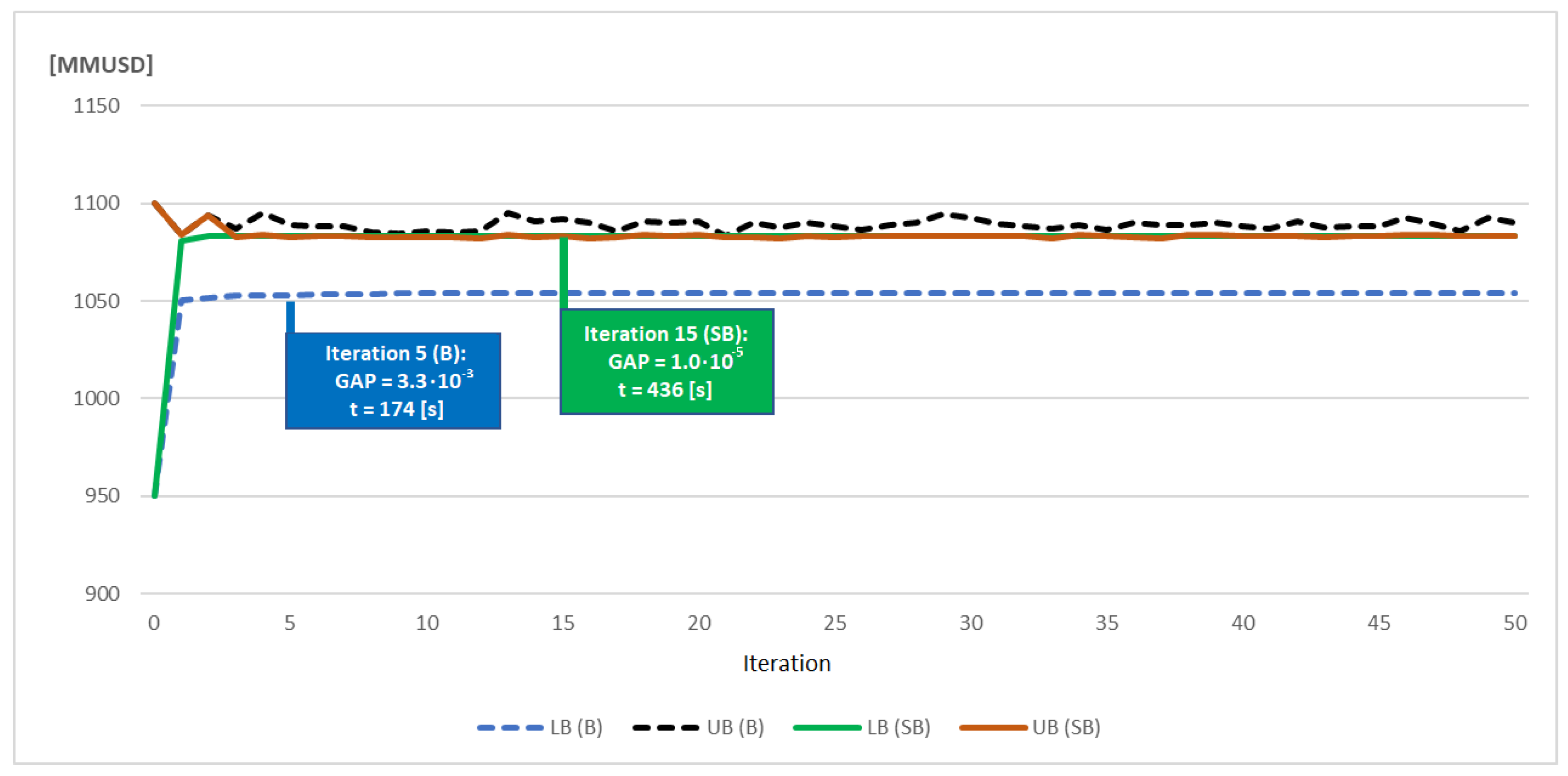
5.1. Results of Case I

Using the EF methodology in the IEEE-6 bus system, the relative gap is reached in 1335 s. The solution value weighted by the three samples is 53,915.2 [MMUSD]. With the IEEE-24 bus system, the EF met the gap in 538 s. The weighted solution value for that system is 1084.6 [1000 MMUSD].

Table 7. Cuts performance for the IEEE test cases. (B), (I), and (SB) stand for Benders, Integer Optimality, and Strengthened Benders, respectively. The symbol * indicates the values at which the gap stabilizes.

(a) IEEE-6 Bus Test System.
Converged	No	No	Yes
Time [s]	(100 *)	-	998
No iterations	50 (8 *)	50	32
Solution value [MMUSD]	48,865.8	6245.0	53,913.8
Relative Gap	11%	85%	0%
(b) IEEE-24 Bus Test System.
Converged	No	No	Yes
Time [s]	(174 *)	-	436
No iterations	50 (5 *)	50	15
Solution value [1000 MMUSD]	1054.3	92.1	1083.2
Relative Gap	3%	89%	0%

summarizes the simulation results using the SDDiP methodology for both power systems testing each type of cut.

In Table 7, instances of non-convergence are observed, which can be primarily attributed to challenges in cut generation within the decomposition methodology applied. In the context of our study, cut generation plays a pivotal role in bridging the master problem with sub-problems, guiding the optimization process towards an effective solution. However, the generation of weak or inefficiently managed cuts can impede this process, resulting in slow convergence or failure to converge. Specifically, in the cases presented, non-convergence can be linked to the inability to generate cuts that adequately constrain the solution space or to the computational burden imposed by an excessive number of non-contributory cuts. This underscores the critical importance of robust cut generation and management strategies, as emphasized in our research, to ensure the successful application of decomposition methodologies in solving complex optimization problems. Thus, from the simulation results, we can conclude the following for each type of cut:

• Benders cuts: This type of cut does not meet the convergence criteria in the two test systems. However, the relative gap stagnates at its final value with a low count of iterations: 11% at iteration 8 after 100 s and 3% at iteration 5 after 174 s. This makes sense because this cut uses linear relaxations of the original problem, which involves more differences in case there are a lot of integer variables. Based on the above, it is proven that this type of cut does not accomplish the tight conditions.
• Integer Optimality cuts: This cut is the fastest to iterate, completing 50 iterations in just 281 s for solving the IEEE-6 bus system. Nevertheless, the relative gap could not get better than 85% and 89% for the first and second power systems, respectively. Despite this type of cut ensuring a feasible solution, using only Integer Optimality cuts would not be enough to obtain an optimal value.
• Strengthened Benders cuts: This is the only type of cut that could meet the convergence criteria. Using the SDDiP methodology, this type of cut reduces the simulation times to 75% and ∼81% than using the EF methodology.

On the one side, using the Strengthened Benders cut would be necessary to reduce the simulation time and lead to an optimal solution. On the other side, it should use the Integer Optimality cuts to ensure a feasible solution because this is the unique cut studied in this work that meets the tightness conditions.

5.2. Results of Case II

The convergence progress of Benders cuts (B) and Strengthened Benders cuts (SB) are presented in Figure 1 for the IEEE-6 bus system, and Figure 2 for the IEEE-24 bus system. The Integer Optimality cuts (I) are omitted due to the big gap.

The results show again that the Benders cuts converged in a few iterations to a better solution. The relative gaps are 11% in the IEEE-6 bus system and 3% in the IEEE-24 bus system. The problem structure could explain this improvement in the gap. On the one hand, the system of six buses has a smaller quantity of candidates for expansion (generation and transmission), so one capacity expansion plan could differ from another by 800 [MMUSD] (cost of a thermal unit). Thus, there are few options to choose from, so the UB (B) is not steady and oscillates around a value. On the other hand, the 24-bus system has more candidates, which makes the problem more flexible as it has more feasible options, making it possible to trade off operational costs with investment ones.

The Strengthened Benders cuts performed better than the other two options. This type of cut could meet the convergence criteria, and its progress along the iterations is smooth. These cuts can reduce the simulation time regarding the EF methodology. Despite being interesting to explore, using them in the SDDiP methodology is unnecessary to ensure a feasible solution.

Therefore, it is proposed to use a pattern of cuts which contains: (1) the Integer Optimality cuts to ensure that the solution is an integer and set an initial solution, and then (2) the Strengthened Benders cuts mainly to reduce the simulation time and meet the convergence criteria. Thus, the patterns always start with an (I) cut and then the (SB) cuts are applied to the formulation.

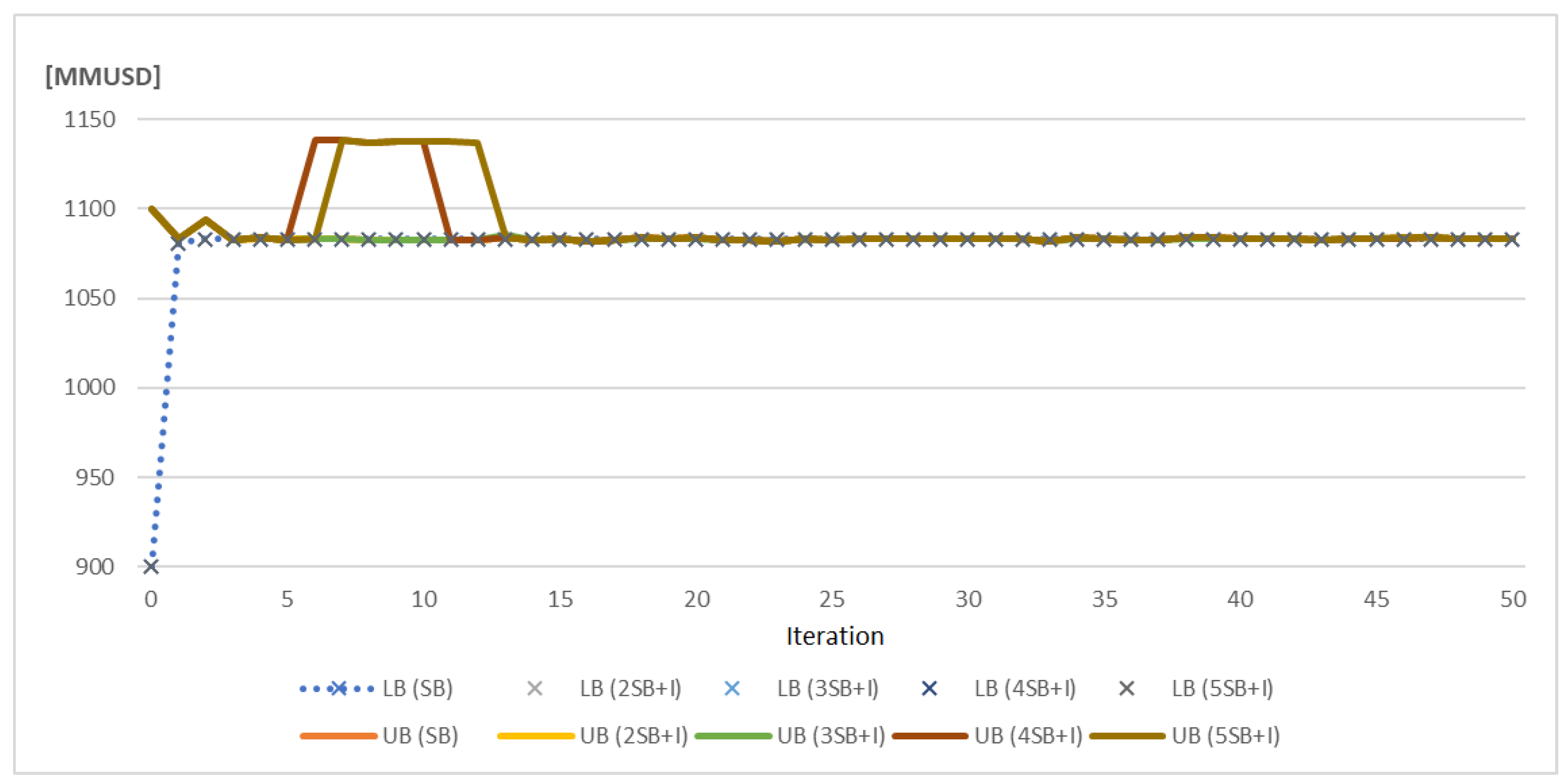
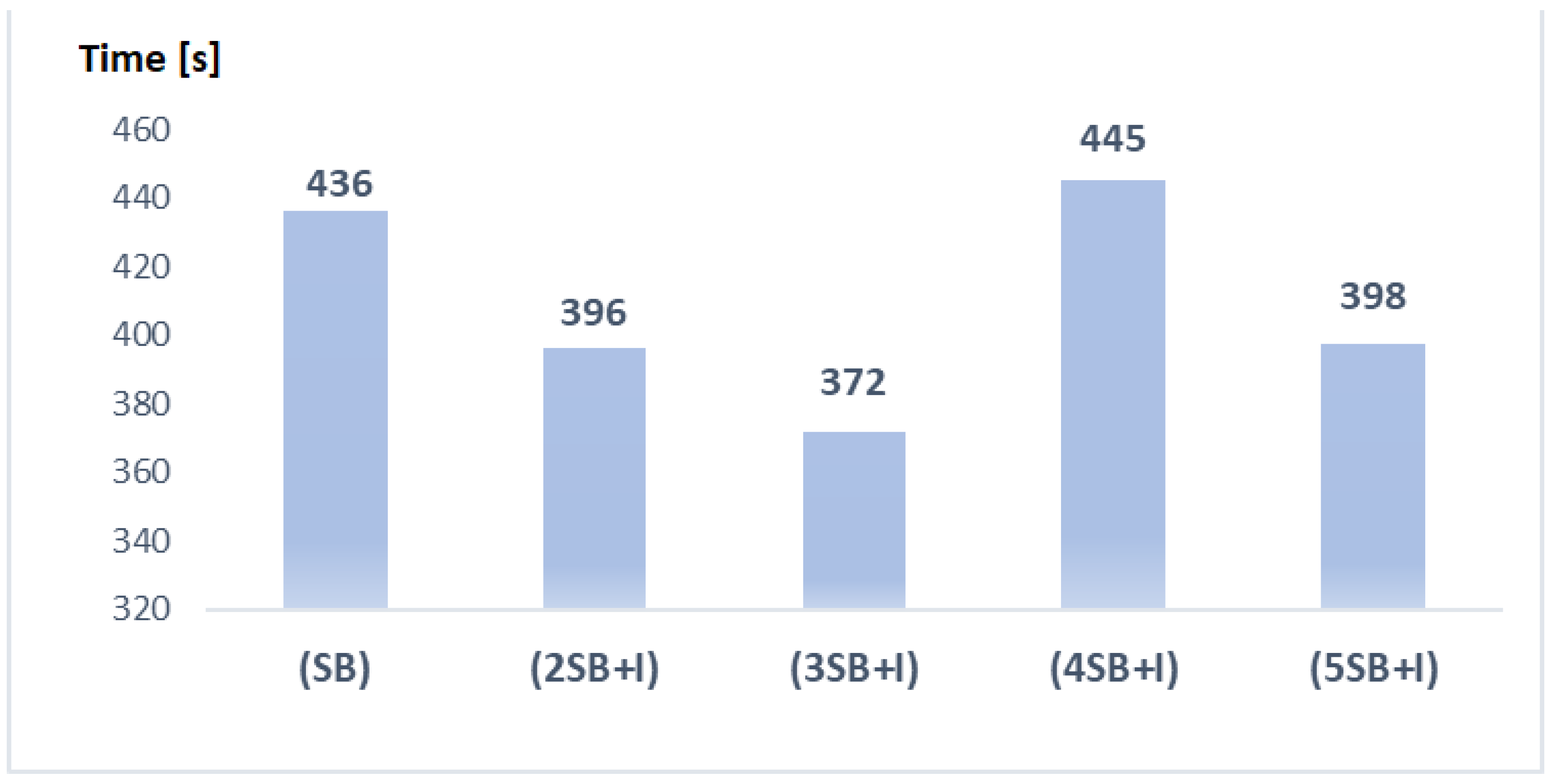
5.3. Results of Case III

Based on the previous study case, the next patterns of cuts are tested:

• 2SB+I: pattern of 3 cuts, where 2 are (SB) and 1 is (I)
• 3SB+I: pattern of 4 cuts, where 3 are (SB) and 1 is (I)
• 4SB+I: pattern of 5 cuts, where 4 are (SB) and 1 is (I)
• 5SB+I: pattern of 6 cuts, where 5 are (SB) and 1 is (I).

The performance results for the patterns of cuts are presented in

Table 8. Simulation information obtained in the IEEE-6 bus system.

Item	SB	2SB+I	3SB+I	4SB+I	5SB+I
Converged	Yes	Yes	Yes	Yes	Yes
Relative Gap	$1.3\times {10}^{-4}$	$1.1\times {10}^{-4}$	$9.7\times {10}^{-5}$	$8.4\times {10}^{-5}$	$1.2\times {10}^{-4}$
Time [s]	998	924	922	1302	1594
No iterations	32	37	33	50	49

for the IEEE-6 bus system. The convergence progress for this system is shown in Figure 3.

As noted, the behavior is similar between patterns of cuts. All patterns reach the convergence criteria between 30 and 50 (maximum allowed) iterations. Using simultaneously the Integer Optimalityand the Strengthened Benderscuts enable us to obtain better signals between stages. (I) cuts give a real estimation of investment costs, then (SB) cuts valorize better the way the integer variables interact with the continuous ones (operational costs because of the investment decisions).

Beyond the completed iterations, it is important to consider the simulation time of each pattern taken to obtain the convergence criteria. Figure 4 compares the run times by each pattern of cuts.

The pattern (2SB+I) improved the simulation time more than using only the Strengthened Benders cuts. Including the Integer Optimality cuts reduced an additional $7\%$ of the simulation time.

Notice that incorporating an additional (SB) cut does not significantly improve the performance (pattern (3SB+I)). This set of cuts had the best performance, reducing the simulation time by 69% compared to the EF methodology.

Adding more (SB) cuts had the opposite effect on the performance. The patterns (4SB+I) and (5SB+I) had the opposite effect on the performance. The simulation time increases. In fact, the pattern (5SB+I) took more time than the EF methodology.

For the IEEE-24 bus system, the performance results by pattern of cuts are presented in

Table 9. Simulation information obtained in the IEEE-24 bus system.

Item	SB	2SB+I	3SB+I	4SB+I	5SB+I
Converged	Yes	Yes	Yes	Yes	Yes
Relative Gap	$2.1\times {10}^{-5}$	$6.0\times {10}^{-5}$	$6.7\times {10}^{-5}$	$7.7\times {10}^{-5}$	$7.7\times {10}^{-5}$
Time [s]	436	396	372	445	398
No iterations	15	15	15	15	15

, and the convergence progress is shown in Figure 5.

For this system, all of the patterns converged at 15 iterations. However, the patterns (4SB+I) and (5SB+I) had a particular behavior mainly when the second Integer Optimality cuts are applied (iterations five and six, respectively). The (UB) increased and was high until the third (I) cuts were used (iterations 11 and 13, respectively). This evidences that working with integer variables could lead to this instability in the convergence if the cut’s application is improper. Based on these achievements, we can conclude that for this system, it is necessary to use a (I) cut before iteration N^o 4.

Figure 6 shows the simulation times by each pattern of cuts for the IEEE-24 bus system.

As with the IEEE-6 bus system, the pattern (3SB+I) performed best. It reduced the simulation time to 69% regarding the EF methodology. Also, the patterns (4SB+I) and (5SB+I) have an adverse effect, proving that having more (SB) cuts on a pattern does not imply better performance.

From the results, we can conclude that the pattern (3SB+I) is the best option for the SDDiP methodology. It met the convergence criteria in less simulation time, reducing up to 69% regarding the EF methodology. In addition, we highlight that patterns (4SB+I) and (5SB+I) are not helpful for this type of problem. Hence, they should be discarded for future planning research.

6. Conclusions and Further Research

This study introduced an efficient cut setting formulation integrating Strengthened Benders and Integer Optimality cuts to address the stochastic capacity expansion planning problem for power systems. Through rigorous simulation across three case studies, we validated the superior performance of the SDDiP methodology over the Extensive Formulation (EF) approach without compromising on convergence and optimality, demonstrating not only its academic merit but also its practical applicability in power system planning.

Our findings highlight the SDDiP methodology’s ability to reduce simulation times significantly. Specifically, the Strengthened Benders cuts demonstrated substantial progress in convergence, achieving completion in 998 s for the IEEE-6 bus system and 436 s for the IEEE-24 bus system, marking reductions of 75% and approximately 81%, respectively, compared to the EF methodology. This reduction is crucial for the dynamic and efficient planning needed in today’s rapidly evolving energy sector. Furthermore, Integer Optimality cuts emerged as the fastest iterating type, though they struggled to significantly improve the low relative gap.

The exploration of cut patterns revealed that a combination of three Strengthened Benders cuts followed by one Integer Optimality cut (3SB+I) not only delivered the most efficient performance but also indicated a practical path forward for implementing such methodologies in large-scale power systems. This pattern ensured optimality and feasibility and reduced simulation times by up to 69% compared to the EF methodology, underlining its potential for practical application in real-world power system planning contexts.

Looking ahead, the promising results from the 3SB+I pattern open avenues for integrating additional variables with long-term operational and investment cost implications, such as fuel contracts or long-term hydro storage. These elements could refine the planning methodology by allowing for more nuanced investment decisions in future energy systems, where decisions must account for long-term operational costs, investment strategies, higher variability, the need for operational flexibility, and environmental sustainability.

In conclusion, our research contributes a novel and effective approach that directly addresses the complexities of large-scale power system planning. The demonstrated effectiveness of our proposed cut patterns, especially 3SB+I, signifies a step forward in addressing the complexities of large-scale power system planning, offering a robust tool for future research and practical applications in the energy sector.

References

1. Peng, Q.; Liu, W.; Shi, Y.; Dai, Y.; Yu, K.; Graham, B. Multi-Objective Electricity Generation Expansion Planning towards Renewable Energy Policy Objectives under Uncertainties. 2023. Available online: https://papers.ssrn.com/sol3/papers.cfm?abstract_id=4584199 (accessed on 1 March 2024).
2. Wei, Z.; Yang, L.; Chen, S.; Ma, Z.; Zang, H.; Fei, Y. A multi-stage planning model for transitioning to low-carbon integrated electric power and natural gas systems. Energy 2022, 254, 124361. [Google Scholar] [CrossRef]
3. Abdin, A.F.; Caunhye, A.; Zio, E.; Cardin, M.A. Optimizing generation expansion planning with operational uncertainty: A multistage adaptive robust approach. Appl. Energy 2022, 306, 118032. [Google Scholar] [CrossRef]
4. Wyrwa, A.; Suwała, W.; Pluta, M.; Raczyński, M.; Zyśk, J.; Tokarski, S. A new approach for coupling the short-and long-term planning models to design a pathway to carbon neutrality in a coal-based power system. Energy 2022, 239, 122438. [Google Scholar] [CrossRef]
5. Li, C.; Conejo, A.J.; Siirola, J.D.; Grossmann, I.E. On representative day selection for capacity expansion planning of power systems under extreme operating conditions. Int. J. Electr. Power Energy Syst. 2022, 137, 107697. [Google Scholar] [CrossRef]
6. Li, C.; Grossmann, I.E. A review of stochastic programming methods for optimization of process systems under uncertainty. Front. Chem. Eng. 2021, 2, 34. [Google Scholar] [CrossRef]
7. Wang, B.; Wang, X.; Wei, F.; Shao, C.; Zhou, J.; Lin, J. Multi-stage stochastic planning for a long-term low-carbon transition of island power system considering carbon price uncertainty and offshore wind power. Energy 2023, 282, 128349. [Google Scholar] [CrossRef]
8. Zhang, H.; Domènech, È.M.; Grossmann, I.E.; Tomasgard, A. Decomposition Methods for Multi-Horizon Stochastic Programming. 2023. Available online: https://www.researchsquare.com/article/rs-3258743/v2 (accessed on 1 March 2024).
9. Hou, S.; Fan, Y.; Yi, B.W. Long-term renewable electricity planning using a multistage stochastic optimization with nested decomposition. Comput. Ind. Eng. 2021, 161, 107636. [Google Scholar] [CrossRef]
10. Li, C.; Conejo, A.J.; Liu, P.; Omell, B.P.; Siirola, J.D.; Grossmann, I.E. Mixed-integer linear programming models and algorithms for generation and transmission expansion planning of power systems. Eur. J. Oper. Res. 2022, 297, 1071–1082. [Google Scholar] [CrossRef]
11. Mazzi, N.; Grothey, A.; McKinnon, K.; Sugishita, N. Benders decomposition with adaptive oracles for large scale optimization. Math. Program. Comput. 2021, 13, 683–703. [Google Scholar] [CrossRef]
12. Zhang, H.; Mazzi, N.; McKinnon, K.; Nava, R.G.; Tomasgard, A. A stabilised Benders decomposition with adaptive oracles applied to investment planning of multi-region power systems with short-term and long-term uncertainty. arXiv 2022, arXiv:2209.03471. [Google Scholar]
13. Zhang, H.; Grossmann, I.E.; Knudsen, B.R.; McKinnon, K.; Nava, R.G.; Tomasgard, A. Integrated investment, retrofit and abandonment planning of energy systems with short-term and long-term uncertainty using enhanced Benders decomposition. arXiv 2023, arXiv:2303.09927. [Google Scholar]
14. Laporte, G.; Louveaux, F.V. The integer L-shaped method for stochastic integer programs with complete recourse. Oper. Res. Lett. 1993, 13, 133–142. [Google Scholar] [CrossRef]
15. Zou, J.; Ahmed, S.; Sun, X.A.; Stewart, H.M. Nested decomposition of multistage stochastic integer programs with binary state variables. Optim. Online 2016, 5436, 34. [Google Scholar]
16. Gil, E.; Aravena, I.; Cárdenas, R. Generation Capacity Expansion Planning Under Hydro Uncertainty Using Stochastic Mixed Integer Programming and Scenario Reduction. IEEE Trans. Power Syst. 2015, 30, 1838–1847. [Google Scholar] [CrossRef]
17. Hinojosa, V.H.; Sepúlveda, J. Solving the Stochastic Generation and Transmission Capacity Planning Problem Applied to Large-Scale Power Systems Using Generalized Shift-Factors. Energies 2020, 13, 3327. [Google Scholar] [CrossRef]
18. Morales-España, G.; Latorre, J.M.; Ramos, A. Tight and compact MILP formulation for the thermal unit commitment problem. IEEE Trans. Power Syst. 2013, 28, 4897–4908. [Google Scholar] [CrossRef]
19. Bertsekas, D. Abstract Dynamic Programming; Athena Scientific: Nashua, NH, USA, 2022. [Google Scholar]
20. Ma, Q.; Stachurski, J. Dynamic programming deconstructed: Transformations of the Bellman equation and computational efficiency. Oper. Res. 2021, 69, 1591–1607. [Google Scholar] [CrossRef]
21. Zou, J.; Ahmed, S.; Sun, X.A. Stochastic dual dynamic integer programming. Math. Program. 2019, 175, 461–502. [Google Scholar] [CrossRef]
22. Benders, J. Partitioning procedures for solving mixed-variables programming problems. Numer. Math. 1962, 4, 238–252. [Google Scholar] [CrossRef]
23. Thomé, F.S. Application of Decomposition Technique with Evaluation of Implicit Multipliers in Electrical Systems Generation and Network Expansion Planning. Ph.D. Thesis, Dissertação de Mestrado, COPPE/UFRJ, Rio de Janeiro, Brazil, 2008. (In Portuguese). [Google Scholar]
24. Zimmerman, R.D.; Murillo-Sánchez, C.E.; Thomas, R.J. MATPOWER: Steady-state operations, planning, and analysis tools for power systems research and education. IEEE Trans. Power Syst. 2010, 26, 12–19. [Google Scholar] [CrossRef]
25. Data Tables. Available online: https://docs.google.com/spreadsheets/d/1L4fbv8qo41Kgz8n9ycY5un7G5JYrbcbeeNKng7zz6yg/ (accessed on 5 October 2023).
26. Bezanson, J.; Edelman, A.; Karpinski, S.; Shah, V.B. Julia: A fresh approach to numerical computing. SIAM Rev. 2017, 59, 65–98. [Google Scholar] [CrossRef]
27. Lubin, M.; Dowson, O.; Garcia, J.D.; Huchette, J.; Legat, B.; Vielma, J.P. JuMP 1.0: Recent improvements to a modeling language for mathematical optimization. Math. Program. Comp. 2023, 15, 581–589. [Google Scholar] [CrossRef]
28. Dowson, O.; Kapelevich, L. SSDDP.jl: A Julia Package for Stochastic Dual Dynamic Programming. INFORMS J. Comp. 2020, 33, 27–33. [Google Scholar] [CrossRef]
Figure 1. Convergence progress for (B) and (SB) cuts obtained in the IEEE 6-bus system.
Energies 17 01509 g001
Figure 2. Convergence progress for (B) and (SB) cuts obtained in the IEEE 24-bus system.
Energies 17 01509 g002
Figure 3. Convergence progress obtained for the IEEE-6 bus.
Energies 17 01509 g003
Figure 4. Simulation times obtained by each pattern in the IEEE-6 bus system.
Energies 17 01509 g004
Figure 5. Convergence progress obtained for the IEEE-24 bus system.
Energies 17 01509 g005
Figure 6. Simulation times obtained by each pattern in the IEEE-24 bus.
Energies 17 01509 g006