Disturbance Observer-Based Robust Cooperative Adaptive Cruise Control Approach under Heterogeneous Vehicle

Abstract

Cooperative adaptive cruise control (CACC) is one of the control methods that improves fuel efficiency by allowing multiple vehicles to drive in groups. In this paper, we propose a robust CACC with a heterogeneous vehicle using a disturbance observer. The longitudinal vehicle dynamics, including the engine dynamics, have been modeled as a first-order model using a time constant. However, the simplified first-order model varies in accuracy depending on the dynamic driving situation due to engine performance and air drag force. Designing a more accurate higher-order model might be a solution, but this has a high computational cost. Thus, we propose an augmented state observer for model uncertainties and disturbances. The proposed method makes it possible to design a CACC using nominal parameters without considering dynamic changes to the model parameters. Also, the proposed method can directly compensate for disturbances, compared to the adaptation technique, while also satisfying string stability. The proposed method was validated via computational simulations for heterogeneous traffic and experimental evaluation.

1. Introduction

In the automotive industry, advanced driver assistance systems (ADASs) have been actively developed to reduce accident risk, improve safety, decrease driver stress while driving, and enhance the comfort and driving performance of a vehicle [1,2,3,4,5]. An adaptive cruise control (ACC) system is an ADAS with environment perception sensors [6,7,8,9]. The ACC maintains a safe distance with a constant time gap (CTG) policy using a vehicle’s environment perception sensors, such as radar and camera [10,11,12]. At the same time, the development of vehicle-to-everything (V2X) communication allows the ACC to use the preceding or adjacent vehicle’s information [13]. Thus, a cooperative ACC (CACC) using a preceding vehicle’s acceleration has recently been developed [14,15]. The advantage of a CACC is that a CACC-equipped vehicle can decrease the constant time headway compared to an ACC [16,17,18]. In other words, the CACC could reduce the length of the platoon by decreasing the distance from an ego vehicle to its preceding vehicle. This CACC technology can improve traffic flow efficiency and reduce driver stress. An optimal ACC method was proposed for homogeneous traffic in [19]. Experimental evaluation of a CACC was also reported in [15,20] using a homogeneous platoon. In [21], a novel definition for string stability was introduced and analyzed for a CACC. A robust model predictive control-based CACC was also proposed in [22,23,24]. Recently, a CACC for heterogeneous traffic has been studied. A frequency-domain approach was also introduced for a string-stable CACC design [18,25]. They presented the criteria for the input, output, and error string stability of the CACC. In [26], they solved the heterogeneous time-varying delay problem using a novel distributed control. The effects of a heterogeneous vehicle’s connectivity structures and information delays were analyzed in [27,28]. Most of the above papers deal with the communication time delay of a heterogeneous vehicle. An adaptation law for an uncertain heterogeneous platoon with unknown engine performance losses was proposed in [29,30], but the proposed method requires adaptation time to converge. In this paper, we propose a disturbance observer for a CACC with a heterogeneous vehicle. The longitudinal vehicle dynamics, including the engine dynamics, have been modeled as a first-order model using a time constant [31]. However, the simplified first-order model varies with the dynamic driving situation due to engine performance and air drag force. Designing a higher-order model to be an accurate model might be the solution, but it has a high computational cost. Thus, we proposed the augmented state observer for model uncertainties and disturbances. The proposed method makes it possible to design the CACC using the nominal parameter without considering any dynamic changes to the model parameters. Also, the proposed method can directly compensate the disturbance compared to the adaptation technique [29,30]. The contributions of this paper are as follows:

• The proposed method gives the design solution for the CACC without considering the varying and unknown parameters of a heterogeneous vehicle.
• The string stability of the CACC is maintained by applying the proposed disturbance observer.
• Vehicle vendors can implement the standard CACC on every heterogeneous vehicle.

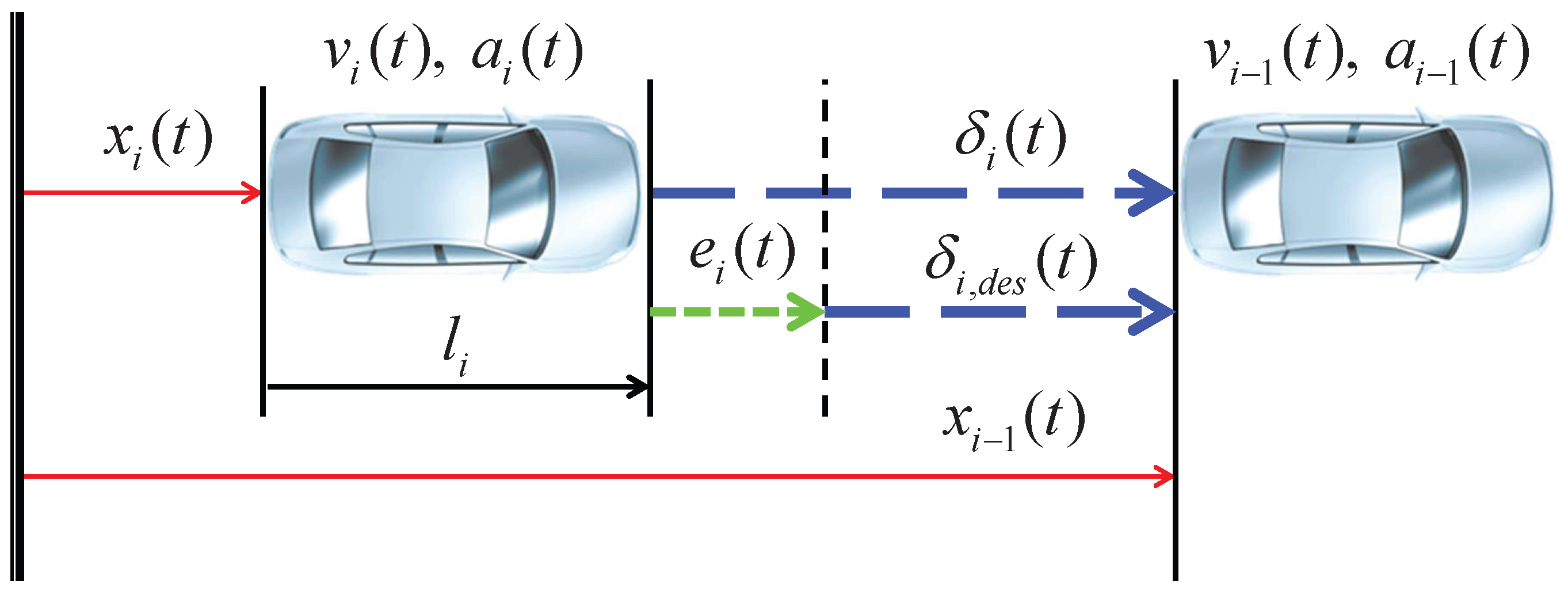
2. System Modeling

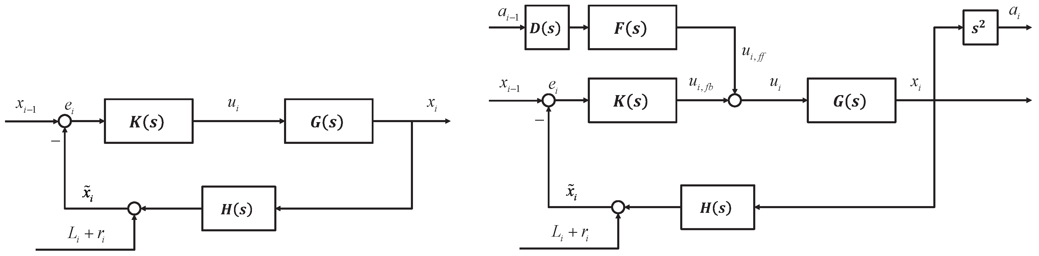
2.1. Adaptive Cruise Control

The longitudinal dynamics of the ego vehicle, ACC, and CACC are described briefly in this section. Definitions of the state in the time domain and parameters for the longitudinal motion are described in Figure 1.

Using the Laplace transform, the vehicle longitudinal dynamics, engine maps, and nonlinear control synthesis techniques can be modeled as the following first-order lag system [31]:

$$\begin{array}{c}\hfill {\displaystyle a_i=\frac{1}{{\tau }_{i}s+1}{u}_i,}\end{array}$$

(1)

where s denotes the Laplace operator and the subscript i denotes the index of the vehicle. $x_i$ denotes the absolute position of the i-th vehicle in global coordinates in the longitudinal direction, $v_i$ and $a_i$ denote the i-th vehicle’s velocity and acceleration in the longitudinal direction, respectively, and $u_i$ denotes the desired acceleration input of the i-th vehicle. The acceleration model with a lag of ${\tau }_i$ results in the following longitudinal equations [13]:

$$\begin{array}{cc}\hfill {\dot{x}}_i& =v_i\hfill \\ \hfill {\dot{v}}_i& =a_i\hfill \\ \hfill {\dot{a}}_i& {\displaystyle =-\frac{1}{{\tau }_i}{a}_i+\frac{1}{{\tau }_i}{u}_i,i\in V_N}\hfill \end{array}$$

(2)

where $V_N=\{i\in \mathbb{N}|1\le i\le N\}$. To maintain the desired distance between the ego vehicle and the preceding vehicle, the constant time gap (CTG) policy, i.e., a constant time headway spacing policy, was introduced [18]:

$$\begin{array}{c}\hfill {\delta }_{i,des}\left(t\right)=r_i+h{v}_i\left(t\right),2\le i\le m,\end{array}$$

(3)

where ${\delta }_{i,des}$ is the desired distance, h is the time headway, and $r_i$ is a constant term that forms the gap between consecutive vehicles at a standstill. The measured distance between two vehicles, ${\delta }_i$ is given by

$$\begin{array}{c}\hfill {\delta }_i\left(t\right)=x_{i-1}\left(t\right)-x_i\left(t\right)-l_i,\end{array}$$

(4)

where $l_i$ is the length of the i-th vehicle. Note that ${\delta }_i$ can be obtained from vehicle environment sensors such as radar and cameras. Now, the spacing error and its derivative are defined as follows:

$$\begin{array}{cc}\hfill e_i\left(t\right)& ={\delta }_i\left(t\right)-{\delta }_{i,des}\left(t\right)\hfill \\ \hfill & =\left(x_{i-1}\left(t\right)-x_i\left(t\right)-l_i\right)-\left(r_i+h{v}_i\left(t\right)\right)\hfill \\ \hfill {\dot{e}}_i\left(t\right)& ={\dot{\delta }}_i\left(t\right)-{\dot{\delta }}_{i,des}\left(t\right)\hfill \\ \hfill & =\left(v_{i-1}\left(t\right)-v_i\left(t\right)\right)-h{a}_i\left(t\right)\hfill \end{array}$$

(5)

One can obtain a state-space representation of Equations (2) and (5) with the state vector ${\mathbf{x}}_i={\left[\begin{array}{ccc}{e}_i& v_i& a_i\end{array}\right]}^T$ and the control input $u_i$:

$${\dot{\mathbf{x}}}_i=\underset{A}{\underbrace{\left[\begin{array}{ccc}0& -1& -h\\ 0& 0& 1\\ 0& 0& -\frac{1}{{\tau }_i}\end{array}\right]}}{\mathbf{x}}_i+\underset{B}{\underbrace{\left[\begin{array}{c}0\\ 0\\ \frac{1}{{\tau }_i}\end{array}\right]}}{u}_i+\underset{B_v}{\underbrace{\left[\begin{array}{c}1\\ 0\\ 0\end{array}\right]}}{v}_{i-1}.$$

(6)

$$\begin{array}{cc}\hfill u_i\left(t\right)& =k_p{e}_i\left(t\right)+k_d{\dot{e}}_i\left(t\right).\hfill \end{array}$$

(7)

Remark 1.

In this paper, we choose the PD gain as $k_p=k_d^2$ to consider both the desired bandwidth and phase margin [18]. In addition, we assume that exactly the same controllers were implemented in heterogeneous traffic, i.e., ${\{k_p,k_d\}}_i={\{k_p,k_d\}}_{i-1}$ for all $i>1$. Also, the time headway h was assumed to have the same value for the heterogeneous vehicle.

Then, the closed-loop system with a PD controller and CTG policy is derived as follows:

$${\dot{\mathbf{x}}}_i=\underset{A^{cl}}{\underbrace{\left[\begin{array}{ccc}0& -1& -h\\ 0& 0& 1\\ \frac{k_p}{{\tau }_i}& -\frac{k_d}{{\tau }_i}& -\frac{1+h{k}_d}{{\tau }_i}\end{array}\right]}}{\mathbf{x}}_i+\underset{B_v^{cl}}{\underbrace{\left[\begin{array}{c}1\\ 0\\ \frac{k_d}{{\tau }_i}\end{array}\right]}}{v}_{i-1}.$$

(8)

The overall structure of the ACC is described in Figure 2 left. Here, the transfer function is given by

$$\begin{array}{cc}\hfill G_i\left(s\right)& {\displaystyle =\frac{X_i\left(s\right)}{U_i\left(s\right)}=\frac{1}{({\tau }_{i}s+1)s^2},}\hfill \\ \hfill K\left(s\right)& =k_p+k_{d}s,\hfill \\ \hfill H\left(s\right)& =hs+1.\hfill \end{array}$$

(9)

2.2. Cooperative Adaptive Cruise Control

In the case of the CACC, the additional feedforward (FF) is considered to decrease the total length of the platoon. The FF term makes the time headway of the CACC theoretically zero [25]. Figure 2 shows the block diagram of the ACC and CACC. The CACC-equipped vehicle can receive the acceleration of the $(i-1)$-$th$ preceding vehicle. To guarantee string stability, which will be discussed in the next section, the following additional control technique is given [25]:

$$\begin{array}{cc}\hfill U_i\left(s\right)& =U_{i,fb}\left(s\right)+U_{i,ff}\left(s\right)\hfill \\ \hfill & =K\left(s\right)E_i\left(s\right)+F_i\left(s\right)D\left(s\right)A_{i-1}\left(s\right).\hfill \end{array}$$

(10)

where $F_i\left(s\right)={\left(H\left(s\right)G_i\left(s\right)s^2\right)}^{-1}$ is designed for the no communication-delay of $D\left(s\right)=1$. Here, the control input of the CACC consists of two term: $u_{i,fb}$ for ACC and $u_{i,ff}$ for CACC, i.e., $u_i\left(t\right)=u_{i,fb}\left(t\right)+u_{i,ff}\left(t\right)$.

$$\begin{array}{cc}\hfill u_i\left(t\right)& =u_{i,fb}\left(t\right)+u_{i,ff}\left(t\right)\hfill \\ \hfill & =k_p{e}_i\left(t\right)+k_d{\dot{e}}_i\left(t\right)+u_{i,ff}\left(t\right)\hfill \end{array}$$

(11)

Applying Equations (11) to (8), the closed-loop system of the CACC is derived as follows:

$${\dot{\mathbf{x}}}_i=\underset{A^{cl}}{\underbrace{\left[\begin{array}{ccc}0& -1& -h\\ 0& 0& 1\\ \frac{k_p}{{\tau }_i}& -\frac{k_d}{{\tau }_i}& -\frac{1+h{k}_d}{{\tau }_i}\end{array}\right]}}{\mathbf{x}}_i\left(t\right)+\underset{B_v^{cl}}{\underbrace{\left[\begin{array}{c}1\\ 0\\ \frac{k_d}{{\tau }_i}\end{array}\right]}}{v}_{i-1}+\underset{B_{ff}}{\underbrace{\left[\begin{array}{c}0\\ 0\\ \frac{1}{{\tau }_i}\end{array}\right]}}{u}_{i,ff}.$$

(12)

3. String Stability Analysis

It is well known that the ACC and CACC should satisfy both the individual stability condition and the string stability condition of a platoon. The individual stabilities of both the ACC and CACC are guaranteed by choosing an appropriate PD control gain in (8) and (12) according to ${\tau }_i$ and the time headway h [19]. In this section, we discuss the string stability of the CACC and robustness for heterogeneous traffic.

3.1. String Stability in the Ideal Case

String stability is defined quite differently in different types of studies. It is easy to find the pros and cons of different analysis methods and definitions of string stability [32]. In this paper, we specifically focus on output string stability, $E_i\left(s\right)/E_{i-1}\left(s\right)$.

Remark 2.

It has already been proven that the input string stability and the error string stability cannot be guaranteed with heterogeneous traffic. However, output string stability is guaranteed for heterogeneous traffic without communication delay if we know the exact engine dynamics of each vehicle [18]. In this paper, we focus on the output string stability of heterogeneous traffic, which may not be guaranteed with an unknown uncertainty of the plant.

The definition of the output string stability transfer function is given by

$$\begin{array}{cc}\hfill {\Lambda }_{X_i}\left(s\right)& {\displaystyle =\frac{X_i\left(s\right)}{X_{i-1}\left(s\right)}.}\hfill \end{array}$$

(13)

The output string stability can be guaranteed with the following necessary condition:

$$\begin{array}{c}\hfill \parallel {\Lambda }_{X_i}{\left(s\right)\parallel }_{\infty }={∥{\displaystyle \frac{X_i}{X_{i-1}}}∥}_{\infty }\le 1.\end{array}$$

(14)

The following transfer function ${\Lambda }_{X,i}^{CACC}\left(s\right)$ for the string stability is obtained from the block diagram of the CACC in Figure 2 with the FF filter described in Equation (10). The communication delay is outside the scope of this paper and given by $D\left(s\right)=1$.

$$\begin{array}{cc}\hfill {\displaystyle {\Lambda }_{X_i}^{CACC}\left(s\right)=\frac{X_i}{X_{i-1}}}& {\displaystyle =\frac{(F\left(s\right)D\left(s\right)s^2+K\left(s\right))G_i\left(s\right)}{1+H\left(s\right)G_i\left(s\right)K\left(s\right)}}\hfill \\ \hfill & {\displaystyle =\frac{\left({\displaystyle \frac{1}{H\left(s\right)G_i\left(s\right)}+K\left(s\right)}\right)G_i\left(s\right)}{1+H\left(s\right)G_i\left(s\right)K\left(s\right)}}\hfill \\ \hfill & {\displaystyle =\frac{1}{H\left(s\right)}.}\hfill \end{array}$$

(15)

Remark 3.

Note that the CACC yields that the time headway can be zero without a communication delay. However, the time delay of V2X communication should be considered in real traffic situations. The value of h in the CACC should be greater than zero but less than that of the ACC in the presence of a time delay. The design criteria for the time headway h and the PD control gain were presented in [18] and included a time delay.

3.2. String Stability with Uncertainty

In practice, the lag of the vehicular system ${\tau }_i$ is different for heterogeneous vehicles. Also, both the system gains ${\xi }_i$ and ${\tau }_i$ vary with dynamic driving conditions, such as road graduation, air drag force, and tire–road friction. Thus, the approximated longitudinal model has an uncertainty of ${\tau }_i={\tau }_{i,o}+\Delta {\tau }_{i,o}$, where ${\tau }_{i,o}$ denotes the nominal value of the plant. Then, the uncertainty should be considered in designing the controller as follows:

$$\begin{array}{cc}\hfill G_i\left(s\right)& =G_{i,o}\left(s\right)+\Delta G_{i,o}\left(s\right)\hfill \\ \hfill & {\displaystyle =\frac{{\xi }_i}{\left(1+({\tau }_{i,o}+\Delta {\tau }_{i,o})s\right)s^2},}\hfill \end{array}$$

(16)

where $G_{i,o}\left(s\right)$ denotes a nominal plant for the controller design and $G_i\left(s\right)$ denotes an actual plant model with uncertainties. The system gain ${\xi }_i$ is equal to one for an ideal system. The FF filter is given by (17) for the nominal plant $G_{i,o}\left(s\right)$, which is different from the FF filter for the actual plant $G_i\left(s\right)$:

$$\begin{array}{cc}\hfill F_i\left(s\right)& {\displaystyle =\frac{1}{H\left(s\right)G_{i,o}\left(s\right)s^2}\ne \frac{1}{H\left(s\right)G_i\left(s\right)s^2}.}\hfill \end{array}$$

(17)

$$\begin{array}{cc}\hfill {\displaystyle \frac{X_i}{X_{i-1}}}& {\displaystyle =\frac{(F\left(s\right)D\left(s\right)s^2+K\left(s\right))G_i\left(s\right)}{1+H\left(s\right)G_i\left(s\right)K\left(s\right)}}\hfill \\ \hfill & {\displaystyle =\frac{\left({\displaystyle \frac{1}{H\left(s\right)G_{i,o}\left(s\right)}+K\left(s\right)}\right)G_i\left(s\right)}{1+H\left(s\right)G_i\left(s\right)K\left(s\right)}}\hfill \\ \hfill & {\displaystyle =\frac{1}{H\left(s\right)}\frac{G_i\left(s\right)}{G_{i,o}\left(s\right)}\frac{1+H\left(s\right)G_{i,o}\left(s\right)K\left(s\right)}{1+H\left(s\right)G_i\left(s\right)K\left(s\right)}}\hfill \end{array}$$

(18)

which is required for designing the controller $K\left(s\right)$ for the unknown uncertainty satisfying string stability. Designing the control gain is quite difficult without prior knowledge of the unknown uncertainty. It is neither easy nor suitable to adjust the control gain after the vendor reveals the vehicle to the market. Thus, we propose a disturbance observer (DOB) scheme for the CACC that allows for uncertainty of the plant. To achieve the desired CACC performance, the DOB can effectively remove the uncertainties directly by using the input and output of the plant, even if an external disturbance exists [33].

4. Robust Cooperative Adaptive Cruise Control

In this section, a disturbance observer (DOB) that can directly compensate for the uncertainty and guarantee string stability of the CACC is described. The block diagram of the proposed DOB for the CACC is described in Figure 3. The DOB possesses the capability to estimate of the full state and disturbance, making it possible to design the controller using full state information [34,35,36,37]. The DOB proposed in this paper immediately gives an estimate of the uncertainty and disturbance [38,39]. Also, the proposed DOB requires only nominal parameters of the plant model for heterogeneous traffic.

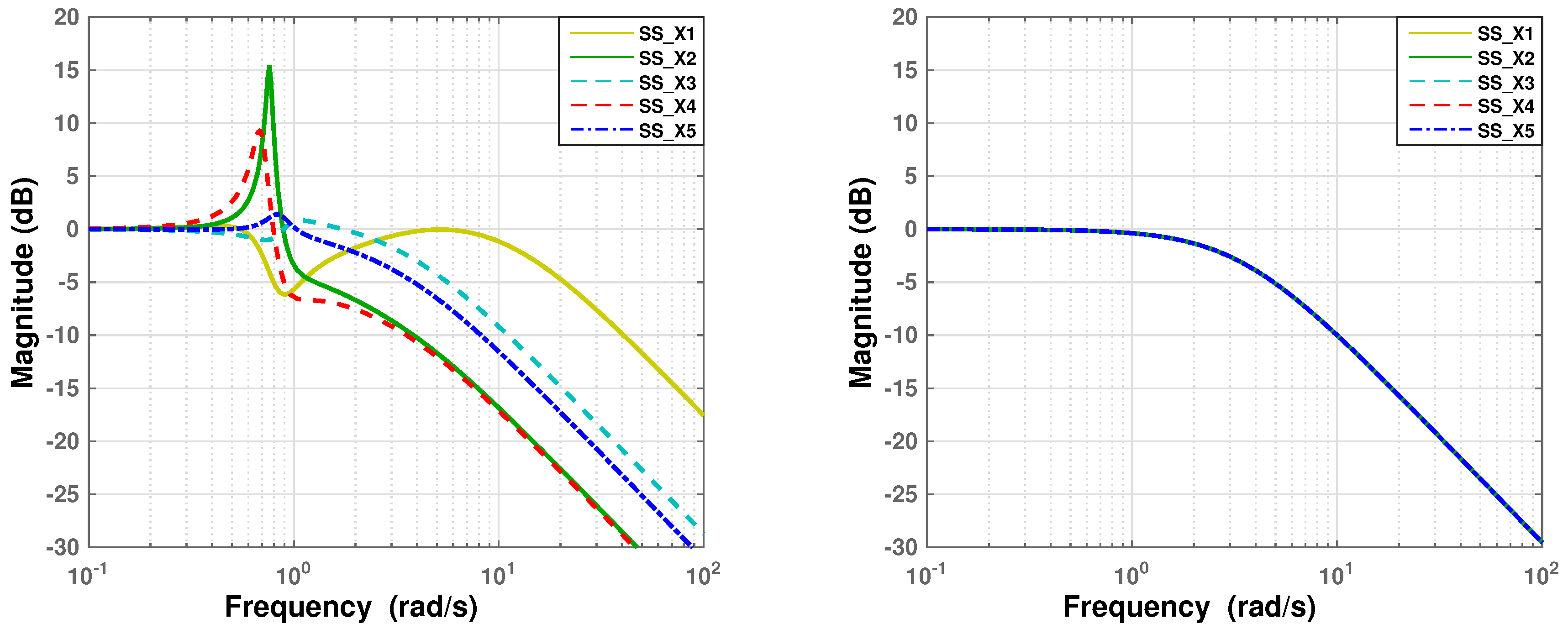
4.1. String Stability with DOB

The string stability of the CACC could be improved by suppressing the influence of the uncertainties with the DOB. The compensated input can be derived from Equation (16). Here, the uncertainty of the transfer function is given by

$$\begin{array}{cc}\hfill \Delta G_{i,o}\left(s\right)& =G_i\left(s\right)-G_{i,o}\left(s\right)\hfill \\ \hfill & {\displaystyle =\frac{{\xi }_i}{\left(1+({\tau }_{i,o}+\Delta {\tau }_{i,o})s\right)s^2}-\frac{1}{\left(1+{\tau }_{i,o}s\right)s^2}}\hfill \\ \hfill & {\displaystyle =\frac{{\xi }_i(1+{\tau }_{i,o}s)-(1+{\tau }_{i}s)}{\left(1+{\tau }_{i}s\right)\left(1+{\tau }_{i,o}s\right)s^2}}\hfill \end{array}$$

(19)

Here, ${\xi }_i$ and $\Delta {\tau }_{i,o}$ denote the unknown system gain and time constant varying with dynamic driving conditions. To compensate for the uncertainty, an additional input $U_{i,d}\left(s\right)$ is designed as follows:

$$\begin{array}{cc}\hfill U_i\left(s\right)-U_{i,d}\left(s\right)& =U_{i,fb}\left(s\right)+U_{i,ff}\left(s\right).\hfill \end{array}$$

(20)

Applying the uncertain system model in (16), the following equation is derived.

$$\begin{array}{c}\hfill {\displaystyle U_i\left(s\right)=\frac{1}{G_{i,o}\left(s\right)+\Delta G_{i,o}\left(s\right)}{X}_i\left(s\right).}\end{array}$$

(21)

The uncertain system in (21) leads to the following equation:

$$\begin{array}{c}\hfill U_i\left(s\right)=\underset{U_{i,o}}{\underbrace{{\displaystyle \frac{X_i\left(s\right)}{G_{i,o}\left(s\right)}}}}-\underset{U_{i,d}}{\underbrace{{\displaystyle \frac{\Delta G_{i,o}\left(s\right)}{G_{i,o}\left(s\right)}{U}_i\left(s\right)}}}\end{array}$$

(22)

where $U_{i,o}$ denotes the input for the nominal plant and $U_{i,d}$ denotes the additional input for the uncertainty. Using the additional input $U_{i,d}$, the uncertain system $G_i\left(s\right)$ converges to $G_{i,o}\left(s\right)$. Then, one can easily obtain the string stability condition of the proposed method (23) from Figure 3:

$$\begin{array}{cc}\hfill {\displaystyle \frac{X_i}{X_{i-1}}}& {\displaystyle =\frac{\left({\displaystyle \frac{1}{H\left(s\right)G_{i,o}\left(s\right)}+K\left(s\right)}\right)G_i\left(s\right)}{1+H\left(s\right)G_i\left(s\right)K\left(s\right)}}\hfill \\ \hfill & {\displaystyle =\frac{\left({\displaystyle \frac{1}{H\left(s\right)G_{i,o}\left(s\right)}+K\left(s\right)}\right)G_{i,o}\left(s\right)}{1+H\left(s\right)G_{i,o}\left(s\right)K\left(s\right)}}\hfill \\ \hfill & {\displaystyle =\frac{1}{H\left(s\right)}}\hfill \end{array}$$

(23)

Equation (23) ensures that the proposed method with the DOB maintains the string stability of the CACC for the nominal plant $G_{i,o}\left(s\right)$. The convergence of the uncertain system will be discussed in the next section.

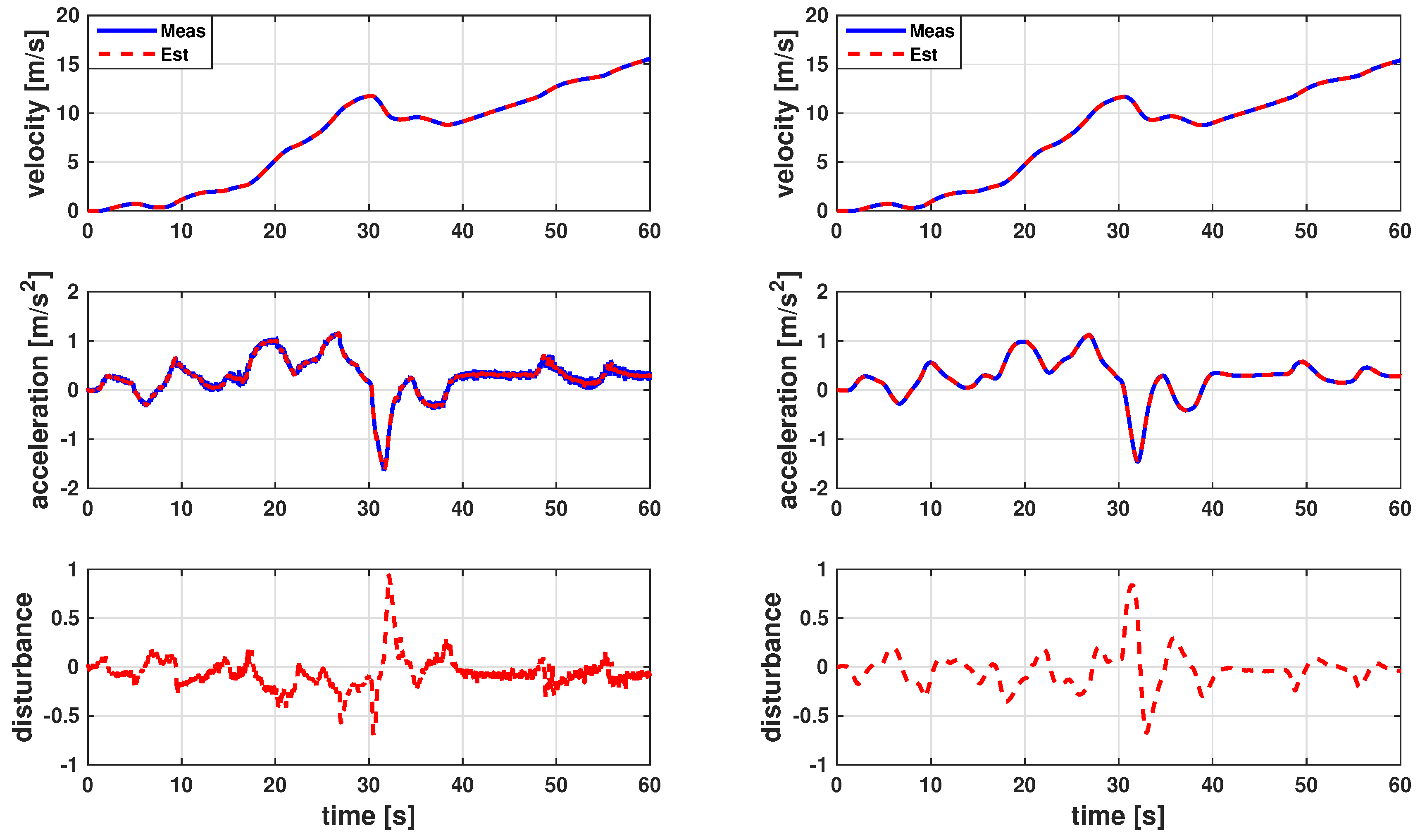
4.2. Convergence of DOB

The system gain ${\xi }_i$ and the lag ${\tau }_i$ are unknown and vary with different driving situations. Thus, the augmented disturbance observer including the uncertainties is designed for the additional input $U_{i,d}$. Equations (19) and (22) show that

$$\begin{array}{cc}\hfill U_{i,d}\left(s\right)& {\displaystyle =\frac{\Delta G_{i,o}\left(s\right)}{G_{i,o}\left(s\right)}{U}_i\left(s\right)}\hfill \\ \hfill & {\displaystyle =\frac{{\xi }_i(1+{\tau }_{i,o}s)-(1+{\tau }_{i}s)}{\left(1+{\tau }_{i}s\right)}{U}_i\left(s\right)}\hfill \\ \hfill & {\displaystyle =\frac{{\xi }_i(1+{\tau }_{i,o}s)-(1+{\tau }_{i}s)}{\xi }{A}_i\left(s\right).}\hfill \end{array}$$

(24)

By taking the inverse Laplace transform, we can calculate additional input $u_{i,d}\left(t\right)$ for the uncertain CACC system and obtain the following Theorem 1.

$$\begin{array}{cc}\hfill u_{i,d}\left(t\right)& {\displaystyle =a_i\left(t\right)-\frac{1}{{\xi }_i}{a}_i\left(t\right)+{\tau }_{i,o}{\dot{a}}_i\left(t\right)-\frac{{\tau }_i}{{\xi }_i}{\dot{a}}_i\left(t\right).}\hfill \end{array}$$

(25)

Assumption 1.

To analyze the string stability of the given CACC, we consider the disturbance at the steady state. The disturbance, $d_i$, is constant or slow varying for an actual system in a steady state. Thus, we can assume that the derivative of the disturbance is ${\dot{d}}_i=0$.

Theorem 1.

Let us consider heterogeneous vehicle traffic including the uncertainties associated with the feedback and feedforward control law $u_i\left(t\right)=k_p{e}_i\left(t\right)+k_d{\dot{e}}_i\left(t\right)+u_{i,ff}\left(t\right)$ as follows:

$$\begin{array}{cc}\hfill {\dot{\mathit{z}}}_i=& \left[\begin{array}{cc}0& 1\\ 0& -\frac{1}{{\tau }_i}\end{array}\right]{\mathit{z}}_i+\left[\begin{array}{c}0\\ \frac{1}{{\tau }_i}\end{array}\right]u_i\hfill \\ \hfill y=& \left[\begin{array}{cc}1& 0\end{array}\right]{\mathit{z}}_i\hfill \end{array}$$

(26)

where the state vector is given by ${\mathit{z}}_i={\left[\begin{array}{cc}{v}_i& a_i\end{array}\right]}^T$. If the following additional compensation input $u_{i,d}$ is applied to each heterogeneous vehicle, then the platoon is string stable for any ${\xi }_i>0$ and ${\tau }_i>0$.

$$\begin{array}{cc}\hfill u_{i,d}\left(t\right)& {\displaystyle =a_i\left(t\right)-\frac{1}{{\xi }_i}{a}_i\left(t\right)+{\tau }_{i,o}{\dot{a}}_i\left(t\right)-\frac{{\tau }_i}{{\xi }_i}{\dot{a}}_i\left(t\right).}\hfill \end{array}$$

(27)

Proof. 

The string stability transfer function derived in (18) is

$$\begin{array}{cc}\hfill {\displaystyle \frac{X_i}{X_{i-1}}}& {\displaystyle =\frac{1}{H\left(s\right)}\frac{G_i\left(s\right)}{G_{i,o}\left(s\right)}\frac{1+H\left(s\right)G_{i,o}\left(s\right)K\left(s\right)}{1+H\left(s\right)G_i\left(s\right)K\left(s\right)}}\hfill \end{array}$$

(28)

for heterogeneous vehicles including uncertainties. The additional compensation input implies that

$$\begin{array}{c}\hfill U_i\left(s\right)+{\widehat{U}}_{i,d}\left(s\right)={\widehat{U}}_{i,o}\left(s\right)={\displaystyle \frac{X_i\left(s\right)}{{\widehat{G}}_{i,o}\left(s\right)}},\end{array}$$

(29)

where ${\widehat{U}}_{i,d},{\widehat{U}}_{i,o}$, and ${\widehat{G}}_{i,o}$ denote estimations of the corresponding variables. To guarantee the string stability, ${\widehat{G}}_{i,o}$ should converge to $G_{i,o}$. The convergence of $G_{i,o}$ can be obtained by showing that ${\widehat{U}}_{i,d}$ converges to $U_{i,d}$. By taking the inverse Laplace transform of $U_{i,d}$ in (24), the additional compensation input $u_{i,d}\left(t\right)=d_i\left(t\right)$ is represented as follows:

$$\begin{array}{cc}\hfill {\dot{a}}_i\left(t\right)& {\displaystyle =-\frac{1}{{\tau }_i}{a}_i\left(t\right)+\frac{{\xi }_i}{{\tau }_i}{u}_i\left(t\right)}\hfill \\ \hfill & {\displaystyle =-\frac{1}{{\tau }_{i,o}}{a}_i\left(t\right)+\frac{1}{{\tau }_{i,o}}(u_i\left(t\right)+d_i\left(t\right)).}\hfill \end{array}$$

(30)

Now, the augmented state-space model with the augmented state vector ${\mathbf{z}}_{i,a}={\left[\begin{array}{ccc}{v}_i& a_i& d_i\end{array}\right]}^T$ is given by

$$\begin{array}{cc}\hfill {\dot{\mathbf{z}}}_{i,a}=& \underset{A_a}{\underbrace{\left[\begin{array}{ccc}0& 1& 0\\ 0& -\frac{1}{{\tau }_{i,o}}& \frac{1}{{\tau }_{i,o}}\\ 0& 0& 0\end{array}\right]}}{\mathbf{z}}_{i,a}+\underset{B_a}{\underbrace{\left[\begin{array}{c}0\\ \frac{1}{{\tau }_{i,o}}\\ 0\end{array}\right]}}{u}_i\hfill \\ \hfill y=& \underset{C_a}{\underbrace{\left[\begin{array}{ccc}1& 0& 0\end{array}\right]}}{\mathbf{z}}_{i,a}.\hfill \end{array}$$

(31)

Since the velocity of the vehicle is more suitable than the acceleration for an observer because of the noise, the measurement matrix is given by $C_a=\left[\begin{array}{ccc}1& 0& 0\end{array}\right]$. From Equation (31), the augmented observer is designed as follows:

$$\begin{array}{c}\hfill {\dot{\widehat{\mathbf{z}}}}_{i,a}=A_a{\widehat{\mathbf{z}}}_{i,a}+B_a{u}_i+L{C}_a({\mathbf{z}}_{i,a}-{\widehat{\mathbf{z}}}_{i,a}),\end{array}$$

(32)

where $L={\left[\begin{array}{ccc}{l}_1& l_2& l_3\end{array}\right]}^T$ is the estimator gain. The estimation error of the augmented state, ${\tilde{\mathbf{z}}}_{i,a}$, is defined as

$$\begin{array}{c}\hfill {\tilde{\mathbf{z}}}_{i,a}={\mathbf{z}}_{i,a}-{\widehat{\mathbf{z}}}_{i,a},\end{array}$$

(33)

and the error dynamics are given by

$$\begin{array}{c}\hfill {\dot{\tilde{\mathbf{z}}}}_{i,a}=\left(A_a-L{C}_a\right){\tilde{\mathbf{z}}}_{i,a}.\end{array}$$

(34)

Here, the observer gains, L, are chosen such that the eigenvalues of the error dynamics, $A_a-L{C}_a$, are in the left-half plane

$$\lambda \left(A_a-L{C}_a\right)\in {\mathbb{C}}^{-}$$

(35)

and all ${\tilde{\mathbf{z}}}_a\in B_z$, where $P_a$ and $Q_a$ are positive definite such that ${(A_a-L{C}_a)}^T{P}_a+P_a(A_a-L{C}_a)+Q_a<0$. Now, the convergence of the augmented states is ensured by choosing the Lyapunov function $V_a$ as follows

$$\begin{array}{c}\hfill V_a={\tilde{\mathbf{z}}}_{i,a}^T{P}_a{\tilde{\mathbf{z}}}_{i,a},\end{array}$$

(36)

where its derivative with respect to time is

$$\begin{array}{cc}\hfill {\dot{V}}_a& ={\tilde{\mathbf{z}}}_{i,a}^T[{(A_a-L{C}_a)}^T{P}_a+P_a(A_a-L{C}_a)]{\tilde{\mathbf{z}}}_{i,a}\hfill \\ \hfill & <{\tilde{\mathbf{z}}}_{i,a}^T[{(A_a-L{C}_a)}^T{P}_a+P_a(A_a-L{C}_a)+Q_a]{\tilde{\mathbf{z}}}_{i,a}\hfill \\ \hfill & <0\hfill \end{array}$$

(37)

The above procedure implies that the estimated nominal plant ${\widehat{G}}_{i,o}$ converges to $G_{i,o}$ as the estimated additional input ${\widehat{u}}_{i,d}$ converges to $u_{i,d}$. Consequently, string stability is guaranteed by satisfying Equation (23). □

Note that Theorem 1 holds even if there is no uncertainty (${\xi }_i=1$ and ${\tau }_{i,o}={\tau }_i$ imply $u_{i,d}=0$).

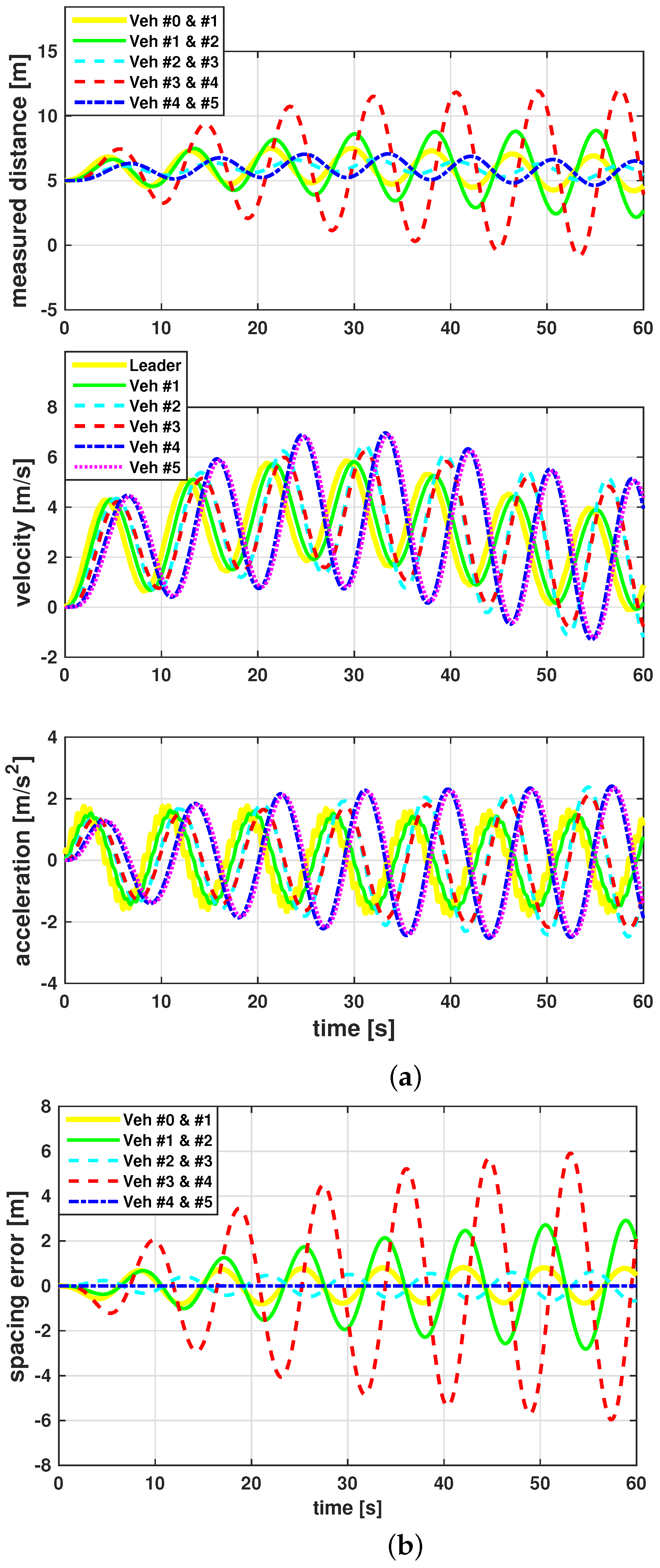
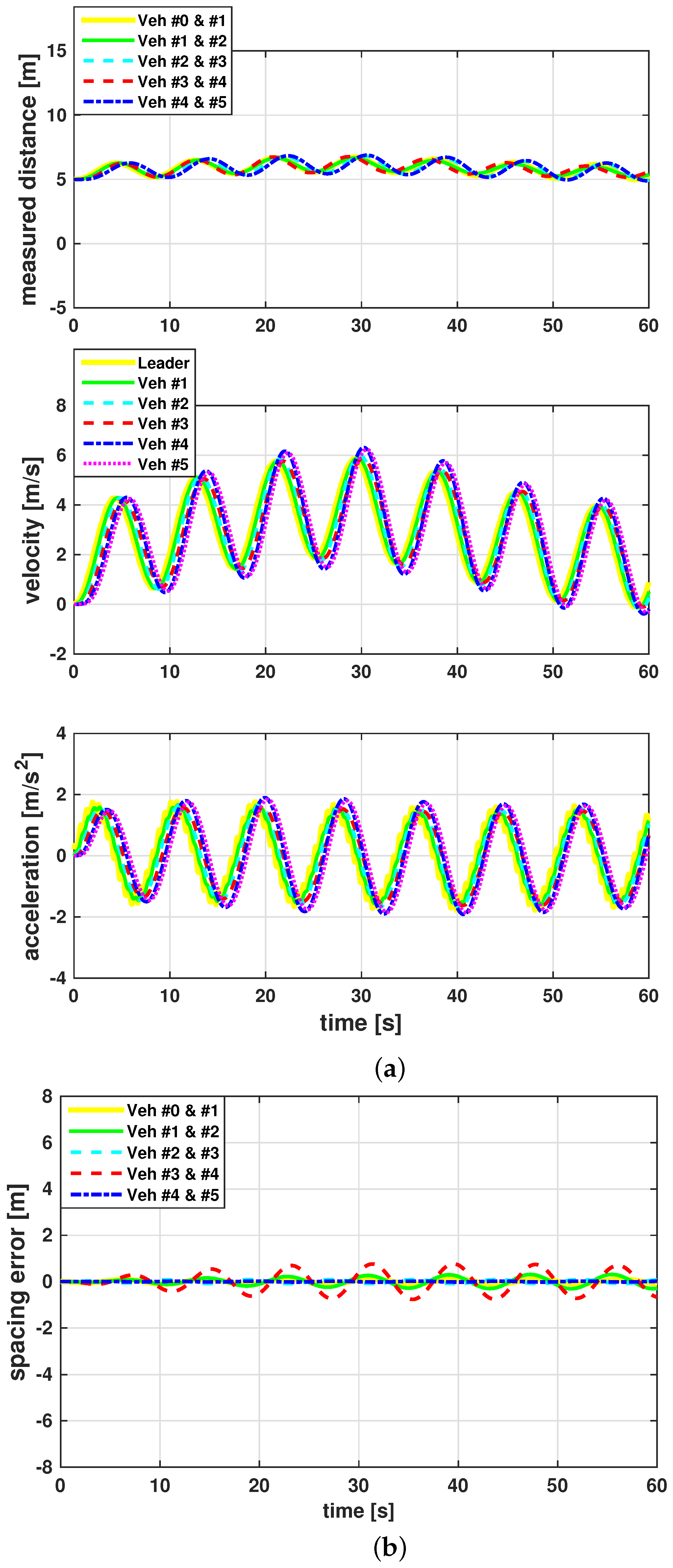
5. Application Results

5.1. Computational Simulation

The proposed method was validated via computational simulation results. To simulate the actual driving situation, three sine waves were combined. This sine combination method is a method that is widely used to check the reference following performance, such as motor control. In addition, we configured a combination of the sine function such that it exists between the acceleration and deceleration limit ranges (−3 m² ≤ a ≤ 2 m²) of the general ACC. The acceleration of the leading vehicle consists of the following three sinusoidal functions:

$$\begin{array}{cc}\hfill y_1\left(t\right)=& 0.1sin\left(0.1t\right)+0.5,\hfill \\ \hfill y_2\left(t\right)=& 0.2sin\left(10t\right)+1,\hfill \\ \hfill y_3\left(t\right)=& 1.5sin\left(0.75t\right).\hfill \end{array}$$

The parameters of heterogeneous traffic are described in

Table 1. Parameters of heterogeneous vehicle.

Number	Initial Position	${\mathit{\tau }}_{\mathit{i}}$	${\mathit{\tau }}_{\mathit{i},\mathit{o}}$	h	$\mathit{\lambda }$
Leader	35	0.5	0.5	0.35	1
$\#1$	30	0.1	0.5	0.35	0.8
$\#2$	25	1	0.5	0.35	0.9
$\#3$	20	0.5	0.5	0.35	1.1
$\#4$	15	0.8	0.5	0.35	0.7
$\#5$	10	0.6	0.5	0.35	1

. We assume that a standard CACC was implemented in each vehicle. Thus, the same time headway $h=0.35$ was selected for a nominal plant ${\tau }_{i,o}=0.5$ for the standard CACC. The standstill distance is set to 5 m. We choose the feedback control gain as $k_d=k_d^2=0.49$ to consider both the bandwidth and phase margin.

The states of the vehicles (${\delta }_i$, $v_i$ and $a_i$) without the DOB are described in Figure 4a. Both the second and fourth vehicles have slow dynamics compared to the preceding vehicles. Also, the parameter ${\tau }_{i,o}$ of the standard CACC is selected to be smaller than ${\tau }_2$, ${\tau }_4$, and ${\tau }_6$. In this case, the desired acceleration of the CACC is not suitable for a vehicle whose dynamics are slower than the nominal plant for designing the CACC (${\tau }_i>{\tau }_{i,o}$). Thus, the magnitude of the fluctuation increases over time and collisions occur after 45 s. The velocity and acceleration show that the vehicle, which differs from the nominal plant, has a critical phase lag. Consequently, the magnitude of the spacing error increases gradually over time in Figure 4b because the error string stability is not guaranteed for heterogeneous traffic. The results of the CACC with the proposed DOB are shown in Figure 5a. The proposed CACC can maintain a standstill distance and exhibits a reduced magnitude of the measured distance because the output string stability is guaranteed. In addition, the phase lags of the velocity and acceleration are reduced to within a small bound. Note that the error string stability is not guaranteed although the proposed DOB is adopted. Nevertheless, the spacing error is regulated with a small bound using the proposed DOB, as shown in Figure 5b.

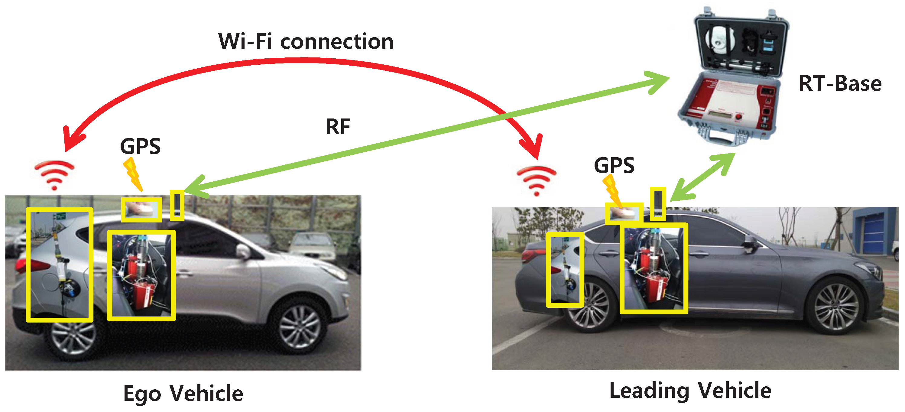
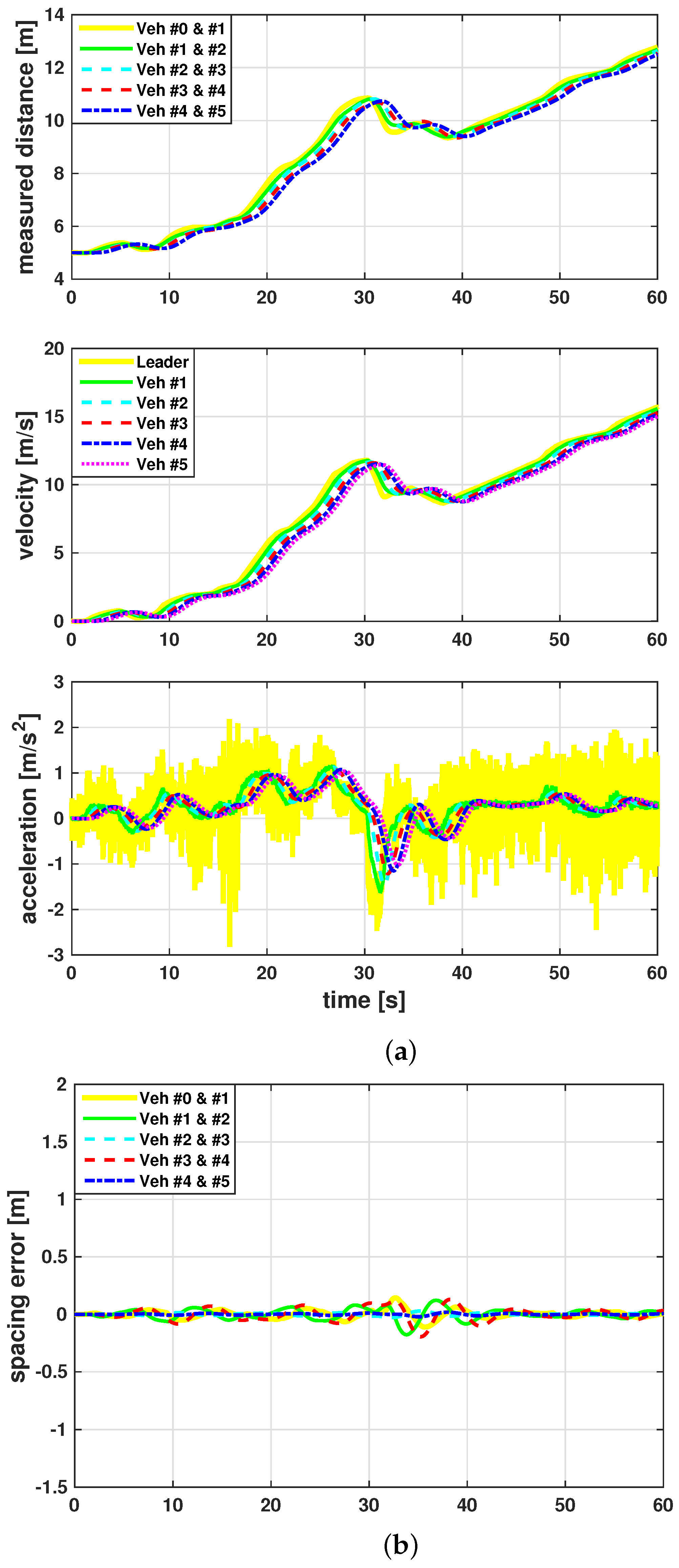
5.2. Experimental Evaluation

A luxury passenger car, GENESIS from HYUNDAI Motors is used for the leading vehicle, which consists of an RT-series (RT-2002, RT-Range, and RT-XLAN) from OxTS [40]. A small sport utility vehicle from HYUNDAI, known as TUCSON, was used as the following vehicle in this experiment, which also consists of an RT-series. RT-2002 was installed in each vehicle and connected with RT-XLAN Wi-Fi using the RT-range from OxTS. The RT-series was installed to obtain the ground truth of the relative distance and the relative velocity between the ego vehicle and the object vehicle using Real-Time Kinematics. The updated sampling rate of the RT-series was 100 Hz. Data analysis was conducted using CANoe from Vector with Kvaser. The overall structure is described in Figure 6. The data were collected via a dSPACE Micro Autobox, and the performance of the proposed method was evaluated in a MATLAB/Simulink (2021b) environment.

The leading vehicle and the following vehicle traveled in the city with real traffic. The leading vehicle’s data, logged at the following vehicle, were considered to be the desired acceleration of the CACC in the MATLAB/Simulink environment. The parameters of heterogeneous traffic are the same as in Table 1.

The relative distance, velocity, and acceleration of the CACC without the DOB are described in Figure 7a. The reference input of the leading vehicle is quite noisy in a real driving situation, which could exacerbate the performance of the CACC. The green line and the red dashed line show the relative distance between the vehicle that has slow dynamics (${\tau }_i>{\tau }_{i,o}$) and the preceding vehicle, which experiences oscillation. Compared to the results with the DOB in Figure 8a, the states are not regulated within a certain bound, and the magnitude of the gap seems to be propagating toward the following vehicle. A bode plot of the output string stability transfer function is shown in Figure 9. The proposed scheme can effectively suppress the influence of the uncertainties satisfying $\parallel {\Lambda }_{X_i}{\left(s\right)\parallel }_{\infty }^{CACC}\le 1$. One can observe that the magnitude of the string stability transfer function never exceeds unity for any uncertainties. We conclude that the proposed CACC scheme can guarantee output string stability and efficiently reduce the spacing error for heterogeneous traffic. Figure 10 shows the estimation results of the proposed augmented state observer. It can be seen that the sign of the disturbance of a vehicle is related to its dynamics. The signs for disturbance of a vehicle with fast dynamics and a vehicle with slow dynamics are opposite one another.

6. Conclusions

In this paper, we propose a robust CACC for heterogeneous traffic. The augmented state observer using a nominal system parameter is designed for a robust CACC. The proposed augmented state observer for model uncertainties and disturbance can effectively reduce the spacing error of the platoon. Further, the proposed method can directly compensate for the disturbance compared to the adaptation technique while satisfying string stability. We expect that the proposed scheme makes it possible to design a uniform robust CACC using the nominal system parameter without considering dynamic changes in the model parameters.

In general, the CACC assumes that the acceleration of the leading vehicle can be received via communication. If the acceleration of the vehicle ahead is not available via communication, the following vehicle can design an estimator that predicts the acceleration of the vehicle ahead using the speed information of the vehicle ahead. Then, one can design the CACC based on the predicted acceleration value. In future works, we will validate the proposed algorithm using a real test vehicle. Also, we will study the CACC’s design in terms of communication interruption.

References

1. Shladover, S.E.; Desoer, C.A.; Hedrick, J.K.; Tomizuka, M.; Walrand, J.; Zhang, W.B.; McMahon, D.H.; Peng, H.; Sheikholeslam, S.; McKeown, N. Automated vehicle control developments in the PATH program. IEEE Trans. Veh. Technol. 1991, 40, 114–130. [Google Scholar] [CrossRef]
2. Wang, J.; Rajamani, R. Adaptive cruise control system design and its impact on highway traffic flow. In Proceedings of the American Control Conference, Anchorage, AK, USA, 8–10 May 2002; Volume 5, pp. 3690–3695. [Google Scholar]
3. Moon, S.; Yi, K. Human driving data-based design of a vehicle adaptive cruise control algorithm. Veh. Syst. Dyn. 2008, 46, 661–690. [Google Scholar] [CrossRef]
4. Xiao, L.; Gao, F. A comprehensive review of the development of adaptive cruise control systems. Veh. Syst. Dyn. 2010, 48, 1167–1192. [Google Scholar] [CrossRef]
5. Batkovic, I.; Zanon, M.; Ali, M.; Falcone, P. Real-time constrained trajectory planning and vehicle control for proactive autonomous driving with road users. In Proceedings of the 2019 18th European Control Conference (ECC), Naples, Italy, 25–28 June 2019; IEEE: Piscataway, NJ, USA, 2019; pp. 256–262. [Google Scholar]
6. Choi, S.B.; Hedrick, J. Vehicle longitudinal control using an adaptive observer for automated highway systems. In Proceedings of the American Control Conference, Seattle, WA, USA, 21–23 June 1995; Volume 5, pp. 3106–3110. [Google Scholar]
7. Swaroop, D.; Hedrick, J.K.; Choi, S.B. Direct adaptive longitudinal control of vehicle platoons. IEEE Trans. Veh. Technol. 2001, 50, 150–161. [Google Scholar] [CrossRef]
8. Vahidi, A.; Eskandarian, A. Research advances in intelligent collision avoidance and adaptive cruise control. IEEE Trans. Intell. Transp. Syst. 2003, 4, 143–153. [Google Scholar] [CrossRef]
9. Bozzi, A.; Zero, E.; Sacile, R.; Bersani, C. Real-time Robust Trajectory Control for Vehicle Platoons: A Linear Matrix Inequality-based Approach. In Proceedings of the ICINCO, Paris, France, 6–8 July 2021; pp. 410–415. [Google Scholar]
10. Hedrick, J.; McMahon, D.; Narendran, V.; Swaroop, D. Longitudinal vehicle controller design for IVHS systems. In Proceedings of the American Control Conference, Boston, MA, USA, 26–28 June 1991; pp. 3107–3112. [Google Scholar]
11. Sheikholeslam, S.; Desoer, C.A. Longitudinal control of a platoon of vehicles with no communication of lead vehicle information: A system level study. IEEE Trans. Veh. Technol. 1993, 42, 546–554. [Google Scholar] [CrossRef]
12. Rajamani, R.; Choi, S.; Law, B.; Hedrick, J.; Prohaska, R.; Kretz, P. Design and experimental implementation of longitudinal control for a platoon of automated vehicles. J. Dyn. Syst. Meas. Control 2000, 122, 470–476. [Google Scholar] [CrossRef]
13. Dey, K.C.; Yan, L.; Wang, X.; Wang, Y.; Shen, H.; Chowdhury, M.; Yu, L.; Qiu, C.; Soundararaj, V. A review of communication, driver characteristics, and controls aspects of cooperative adaptive cruise control (CACC). IEEE Trans. Intell. Transp. Syst. 2016, 17, 491–509. [Google Scholar] [CrossRef]
14. Öncü, S.; Ploeg, J.; van de Wouw, N.; Nijmeijer, H. Cooperative adaptive cruise control: Network-aware analysis of string stability. IEEE Trans. Intell. Transp. Syst. 2014, 15, 1527–1537. [Google Scholar] [CrossRef]
15. Ploeg, J.; Scheepers, B.T.; Van Nunen, E.; Van de Wouw, N.; Nijmeijer, H. Design and experimental evaluation of cooperative adaptive cruise control. In Proceedings of the IEEE International Conference on Intelligent Transportation Systems, Washington, DC, USA, 5–7 October 2011; IEEE: Piscataway, NJ, USA, 2011; pp. 260–265. [Google Scholar]
16. Xu, Q.; Sengupta, R. Simulation, analysis, and comparison of ACC and CACC in highway merging control. In Proceedings of the IEEE Intelligent Vehicles Symposium, Columbus, OH, USA, 9–11 June 2003; pp. 237–242. [Google Scholar]
17. Van Arem, B.; Van Driel, C.J.; Visser, R. The impact of cooperative adaptive cruise control on traffic-flow characteristics. IEEE Trans. Intell. Transp. Syst. 2006, 7, 429–436. [Google Scholar] [CrossRef]
18. Naus, G.J.; Vugts, R.P.; Ploeg, J.; van de Molengraft, M.J.; Steinbuch, M. String-stable CACC design and experimental validation: A frequency-domain approach. IEEE Trans. Veh. Technol. 2010, 59, 4268–4279. [Google Scholar] [CrossRef]
19. Liang, C.Y.; Peng, H. Optimal adaptive cruise control with guaranteed string stability. Veh. Syst. Dyn. 1999, 32, 313–330. [Google Scholar] [CrossRef]
20. Nieuwenhuijze, M.R.; van Keulen, T.; Oncü, S.; Bonsen, B.; Nijmeijer, H. Cooperative driving with a heavy-duty truck in mixed traffic: Experimental results. IEEE Trans. Intell. Transp. Syst. 2012, 13, 1026–1032. [Google Scholar] [CrossRef]
21. Ploeg, J.; Van De Wouw, N.; Nijmeijer, H. Lp string stability of cascaded systems: Application to vehicle platooning. IEEE Trans. Control Syst. Technol. 2014, 22, 786–793. [Google Scholar] [CrossRef]
22. Massera Filho, C.; Terra, M.H.; Wolf, D.F. Safe Optimization of Highway Traffic with Robust Model Predictive Control-Based Cooperative Adaptive Cruise Control. IEEE Trans. Intell. Transp. Syst. 2017, 18, 3193–3203. [Google Scholar] [CrossRef]
23. Graffione, S.; Bersani, C.; Sacile, R.; Zero, E. Non-linear mpc for longitudinal and lateral control of vehicle’s platoon with insert and exit manoeuvres. In Proceedings of the International Conference on Informatics in Control, Automation and Robotics, Paris, France, 7–9 July 2020; Springer: Berlin/Heidelberg, Germany, 2020; pp. 497–518. [Google Scholar]
24. Hult, R.; Zanon, M.; Gros, S.; Falcone, P. Optimal coordination of automated vehicles at intersections: Theory and experiments. IEEE Trans. Control Syst. Technol. 2018, 27, 2510–2525. [Google Scholar] [CrossRef]
25. Naus, G.; Vugts, R.; Ploeg, J.; Van de Molengraft, M.; Steinbuch, M. Towards on-the-road implementation of cooperative adaptive cruise control. In Proceedings of the 16th World Congress and Exhibition on Intelligent Transport Systems and Services, Stockholm, Sweden, 21–25 September 2009. [Google Scholar]
26. Di Bernardo, M.; Salvi, A.; Santini, S. Distributed consensus strategy for platooning of vehicles in the presence of time-varying heterogeneous communication delays. IEEE Trans. Intell. Transp. Syst. 2015, 16, 102–112. [Google Scholar] [CrossRef]
27. Zhang, L.; Orosz, G. Motif-based design for connected vehicle systems in presence of heterogeneous connectivity structures and time delays. IEEE Trans. Intell. Transp. Syst. 2016, 17, 1638–1651. [Google Scholar] [CrossRef]
28. Jin, I.G.; Orosz, G. Dynamics of connected vehicle systems with delayed acceleration feedback. Transp. Res. Part C Emerg. Technol. 2014, 46, 46–64. [Google Scholar]
29. Harfouch, Y.A.; Yuan, S.; Baldi, S. An Adaptive Switched Control Approach to Heterogeneous Platooning with Inter-Vehicle Communication Losses. IEEE Trans. Control Netw. Syst. 2017, 5, 1434–1444. [Google Scholar] [CrossRef]
30. Harfouch, Y.A.; Yuan, S.; Baldi, S. An Adaptive Approach to Cooperative Longitudinal Platooning of Heterogeneous Vehicles with Communication Losses. In Proceedings of the 20th IFAC World Congress, Toulouse, France, 17 July 2017; pp. 1382–1387. [Google Scholar]
31. Rajamani, R. Vehicle Dynamics and Control; Springer: Berlin/Heidelberg, Germany, 2011. [Google Scholar]
32. Feng, S.; Zhang, Y.; Li, S.E.; Cao, Z.; Liu, H.X.; Li, L. String stability for vehicular platoon control: Definitions and analysis methods. Annu. Rev. Control 2019, 47, 81–97. [Google Scholar] [CrossRef]
33. Franklin, G.F.; Powell, J.D.; Workman, M.L. Digital Control of Dynamic Systems; Addison-Wesley: Menlo Park, CA, USA, 1998; Volume 3. [Google Scholar]
34. White, M.T.; Tomizuka, M.; Smith, C. Improved track following in magnetic disk drives using a disturbance observer. IEEE/ASME Trans. Mechatron. 2000, 5, 3–11. [Google Scholar] [CrossRef]
35. Li, S.; Yang, J.; Chen, W.H.; Chen, X. Generalized extended state observer based control for systems with mismatched uncertainties. IEEE Trans. Ind. Electron. 2012, 59, 4792–4802. [Google Scholar] [CrossRef]
36. Ginoya, D.; Shendge, P.; Phadke, S. Sliding mode control for mismatched uncertain systems using an extended disturbance observer. IEEE Trans. Ind. Electron. 2014, 61, 1983–1992. [Google Scholar] [CrossRef]
37. Sun, Z.; Zhang, Z.; Tsao, T.C. Trajectory tracking and disturbance rejection for linear time-varying systems: Input/output representation. Syst. Control Lett. 2009, 58, 452–460. [Google Scholar] [CrossRef]
38. Kim, W.; Shin, D.; Won, D.; Chung, C.C. Disturbance-observer-based position tracking controller in the presence of biased sinusoidal disturbance for electrohydraulic actuators. IEEE Trans. Control Syst. Technol. 2013, 21, 2290–2298. [Google Scholar] [CrossRef]
39. Kim, W.; Shin, D.; Chung, C.C. Microstepping using a disturbance observer and a variable structure controller for permanent-magnet stepper motors. IEEE Trans. Ind. Electron. 2013, 60, 2689–2699. [Google Scholar] [CrossRef]
40. RTv2 GNSS-Aided Inertial Measurement Systems User Manual. 2015. Available online: https://www.oxts.com/app/uploads/2018/02/rtman.pdf (accessed on 25 February 2024).
Figure 1. Definition of state and error.
Energies 17 01429 g001
Figure 2. Block diagram of ACC and CACC. Left: adaptive cruise control (ACC), Right: cooperative adaptive cruise control (CACC).
Energies 17 01429 g002
Figure 3. Block diagram of the proposed DOB-based CACC.
Energies 17 01429 g003
Figure 4. Results of CACC without DOB. The negative value of the measured distance implies a collision. The magnitudes of velocity and acceleration are quite different from each other. Also, the magnitude of the spacing error increases gradually over time. (a) States of vehicles ( δ i , v i and a i ). The measured distance can be obtained from radar or camera vision sensors. The velocity and acceleration of each vehicle are obtained from in-vehicle sensors, respectively, and (b) spacing error for each vehicle e i = δ i , d e s δ i .
Energies 17 01429 g004
Figure 5. Results of CACC with the proposed DOB. The magnitude of the measured distance is reduced without collision. The velocity and acceleration are regulated within a small range. The magnitude of the spacing error is bounded and smaller than that for CACC without DOB. (a) States of vehicles ( δ i , v i and a i ). The measured distance can be obtained from radar or camera vision sensors. The velocity and acceleration of each vehicle are obtained from in-vehicle sensors, respectively, and (b) spacing error for each vehicle e i = δ i , d e s δ i .
Energies 17 01429 g005
Figure 6. Hardware setup for CACC. The data were collected at the ego vehicle via Wi-Fi communication using RT-series. Both the leading vehicle and following vehicle traveled in the city with real traffic.
Energies 17 01429 g006
Figure 7. Results of CACC without DOB using the experimental dataset. The negative value of the measured distance implies a collision. The magnitudes of velocity and acceleration are quite different from each other. Also, the magnitude of the spacing error increases gradually over time. (a) States of vehicles ( δ i , v i and a i ). The measured distance can be obtained from radar or camera vision sensors. The velocity and acceleration of each vehicle are obtained from in-vehicle sensors, respectively, and (b) spacing error for each vehicle e i = δ i , d e s δ i .
Energies 17 01429 g007
Figure 8. Results of CACC with the proposed DOB using the experimental dataset. The magnitude of the measured distance is reduced without a collision. The velocity and acceleration are regulated within a small range. The magnitude of the spacing error is bounded and smaller than that for CACC without DOB. (a) States of vehicles ( δ i , v i and a i ). The measured distance can be obtained from radar or camera vision sensors. The velocity and acceleration of each vehicle are obtained from in-vehicle sensors, respectively, and (b) spacing error of each vehicle e i = δ i , d e s δ i .
Energies 17 01429 g008
Figure 9. Bode plot of the output string stability transfer function. The left figure shows that output string stability is not guaranteed for heterogeneous traffic without DOB. Meanwhile, the right figure shows that output string stability is guaranteed with the proposed DOB.
Energies 17 01429 g009
Figure 10. Estimation results of the proposed augmented state observer. Left: augmented state of vehicle #1; right: augmented stated of vehicle #2.
Energies 17 01429 g010