Centralized vs. Decentralized Electric Grid Resilience Analysis Using Leontief’s Input–Output Model

Abstract

Escalating events such as extreme weather conditions, geopolitical incidents, acts of war, cyberattacks, and the intermittence of renewable energy resources pose substantial challenges to the functionality of global electric grids. Consequently, research on enhancing the resilience of electric grids has become increasingly crucial. Concurrently, the decentralization of electric grids, driven by a heightened integration of distributed energy resources (DERs) and the imperative for decarbonization, has brought about significant transformations in grid topologies. These changes can profoundly impact flexibility, operability, and reliability. However, there is a lack of research on the impact of DERs on the electric grid’s resilience, as well as a simple model to simulate the impact of any disturbance on the grid. Hence, to analyze the electric grid’s resilience, this study employs an extrapolation of Leontief’s input–output (IO) model, originally designed to study ripple effects in economic sectors. Nodes are treated as industries, and power transmission between nodes is considered as the relationship between industries. Our research compares operability changes in centralized, partially decentralized, and fully decentralized grids under identical fault conditions. Using grid inoperability as a key performance indicator (KPI), this study tests the three grid configurations under two fault scenarios. The results confirm the efficacy of decentralization in enhancing the resilience and security of electric grids.

1. Introduction

Modern electric power supply systems are governed by three key criteria: quantity, quality, and reliability. Quantity involves maintaining a balance between power generation and demand, while quality ensures that supplied electricity aligns with predefined characteristics such as voltage and frequency. Reliability, a crucial aspect, is defined as the consistent delivery of electricity without interruption or significant fluctuations, requiring stable flow, demand-meeting power generation, and minimal disruptions from various factors. Grid resilience is a fundamental element in ensuring the reliability of electric grids. It is characterized by the grid’s ability to endure and recover from various disruptions or unforeseen events, such as natural disasters, cyberattacks, or equipment failures [1]. This resilience encompasses the grid’s capacity to absorb shocks, adapt to dynamic conditions, and swiftly restore power following an outage. Strategies to enhance grid resilience often involve leveraging diverse energy sources, establishing a robust infrastructure, and implementing rapid response mechanisms. In contrast, reliability primarily aims to prevent disruptions and maintain an uninterrupted power supply.

Grid resilience has become paramount in the contemporary energy landscape due to heightened reliance on electricity across all economic sectors. The interdependency of critical infrastructures, particularly electricity, communications, healthcare, and transportation [2], further underscores the significance of prioritizing grid resilience. Additionally, national security and independence concerns accentuate the urgency of ensuring grid resilience. Consequently, policymakers, utility companies, and governments worldwide have prioritized fortifying the resilience of electric grids [3].

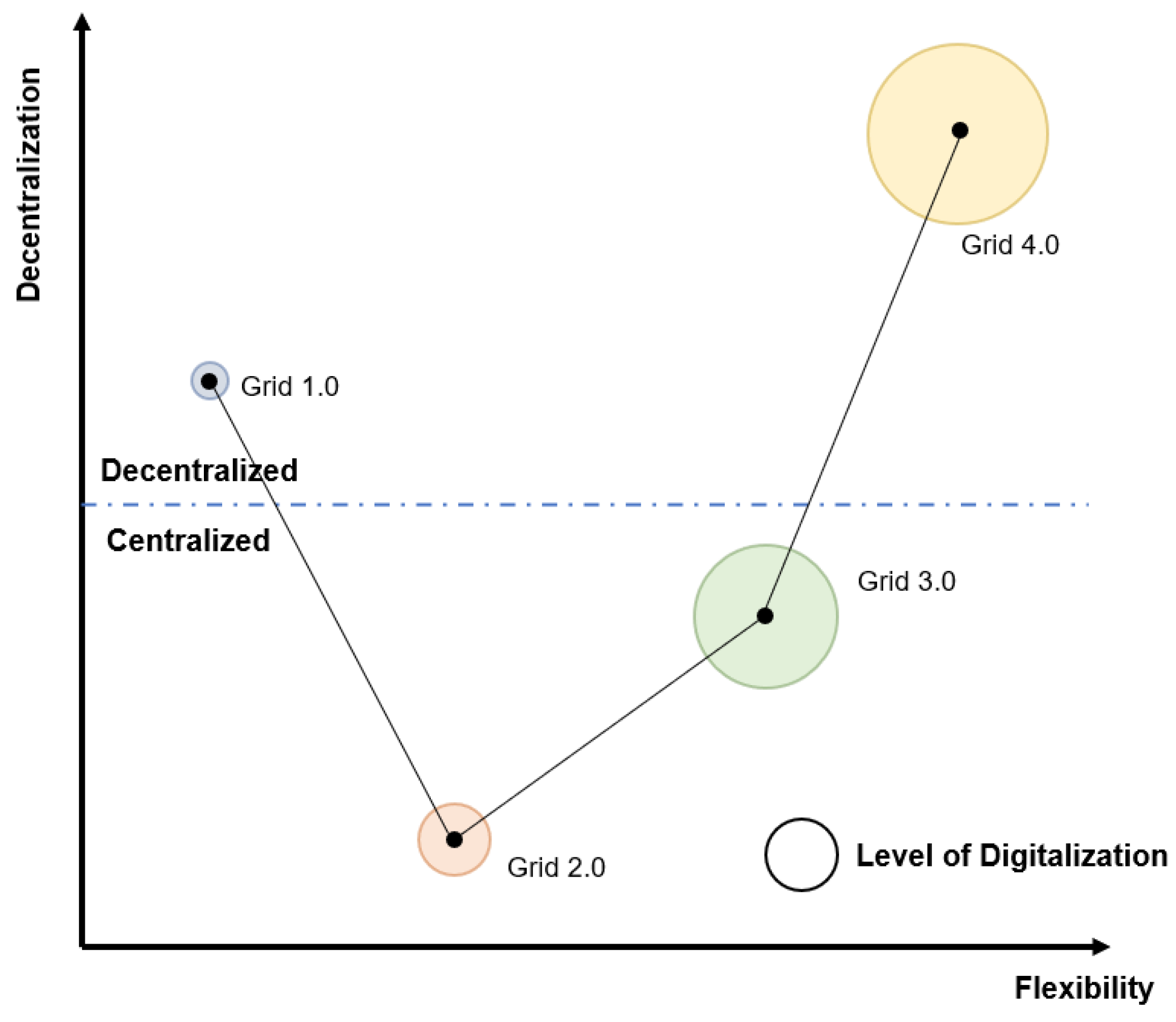
Electric grids originated in the late 19th century as small-scale, primitive, and isolated town-based networks (Grid 1.0). However, driven by a growing reliance on electric power and a substantial surge in energy demand, electric grids evolved into national, large-scale centralized power grids centered around significant power plants (Grid 2.0). A new transformation occurred in less than a century, spurred by the imperative to decarbonize the energy sector. This shift, driven by the increasing integration of renewable energy (RE) systems and DERs, led to a decentralized topology (Grid 3.0).

Today, with the advent of advanced technologies such as artificial intelligence (AI), the blockchain, the Internet of Things (IoT), and the incorporation of concepts like peer-to-peer (P2P) energy trading, energy democracy, and virtual power plants (VPP), the grid is progressing towards complete decentralization, shaping the vision of the future grid (Grid 4.0) as a composite of thousands or even millions of microgrids. Simultaneously, these transformations in the electric grid’s topology align with a surge in digitalization. Recognizing the necessity to address evolving needs and challenges, a core digital transformation occurred at the grid’s operational and asset management levels. The integration of smart metering, advanced metering infrastructure (AMI), and the application of digital technologies for automation and optimization underlined the digital revolution in the electric grid [4]. Undoubtedly, the evolution of the electric grid into a decentralized, highly digitized network significantly enhanced its operational flexibility. Figure 1 depicts the progression of the grid’s topology, digitalization, and flexibility.

However, within the domain of grid resilience, ongoing discourse and analysis revolve around the advantages and disadvantages of centralized and decentralized approaches. Centralized approaches to grid resilience adopt a centralized control architecture, where decisions and actions are coordinated and executed by a central authority or operator. This approach provides superior controllability and predictability, facilitating efficient resource management and response to disruptions. Nonetheless, centralized networks have a notable drawback, known as a single point of failure (SPOF). This refers to a specific grid element, such as a control center, power station, or transmission line, whose failure can significantly disrupt or potentially collapse the entire grid’s functionality. Essentially, it represents a vulnerability that, if compromised, could result in widespread power outages or disruptions [5].

Conversely, decentralized approaches to grid resilience embrace near-edge solutions, including small-scale power generation and energy storage systems [6]. This decentralized architecture provides a heightened level of scalability, allowing for greater flexibility. Additionally, decentralized systems have demonstrated increased resilience in the face of climate-related risks such as wildfires and extreme storm events. Distributed energy systems can effectively mitigate damage or disruption to primary utility components by leveraging end-user solutions like small generators, rooftop solar photovoltaic (PV) systems, and battery energy storage systems (BESS), enhancing overall resilience.

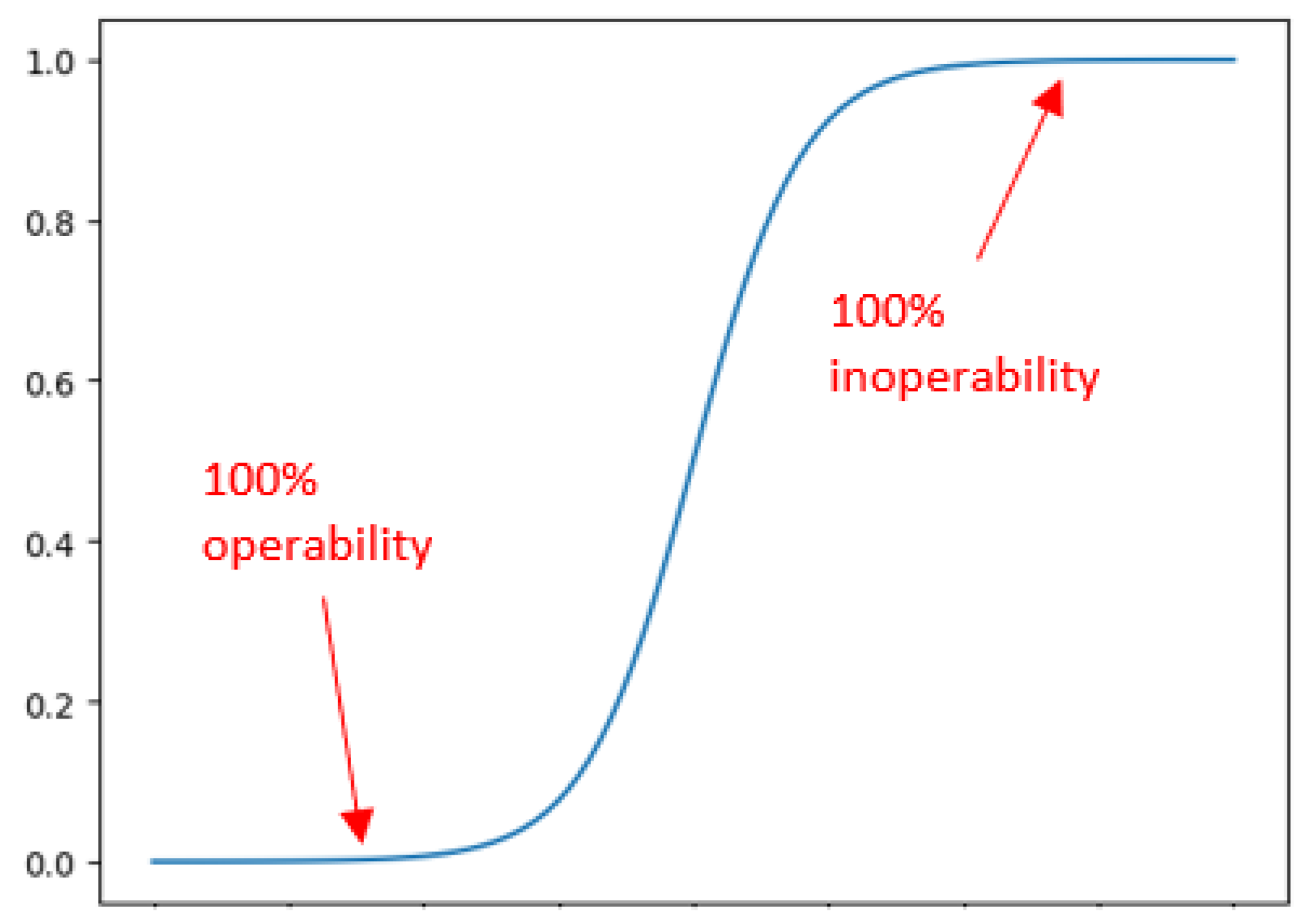
This article explores the impact of electric grid decentralization from a resilience perspective. However, assessing a grid’s resilience necessitates the establishment of a KPI to gauge the effectiveness or inefficiency of a particular solution. In this study, we adopted inoperability as an indicator to assess the resilience health status of each node in the grid. Inoperability is defined as the ratio of the power decline at a specific node following a detected interruption to the baseline power level or essentially business as usual. Consequently, an inoperability value of zero signifies that the node was unaffected by the interruption, while a value of one indicates a complete loss of power at the node (Figure 2).

However, the intricate interconnections among nodes in an electric grid can complicate the measurement of inoperability. Additionally, these interactions, referred to as power transmissivity between nodes, may trigger a chain reaction in the event of a power failure or fault affecting any node. Hence, the need arises for a mathematical model capable of simulating the interconnections between nodes and assessing the impact of any incident on other grid elements. Consequently, we opted to employ Leontief’s IO analysis, a model initially introduced by Wassily Leontief in the 1930s to analyze the interdependencies between different sectors of an economy [7].

In this study, we construct a matrix of interdependency among various components of an electric grid, employing the power transmitted between nodes as a parameter. Subsequently, we apply Leontief’s inoperability input–output model (IIM) to quantify the inoperability of each node. The calculated inoperability serves as a KPI for assessing the grid’s resilience and gauging the repercussions of any incidents, failures, or interruptions in the grid. The proposed mathematical model for calculating the electric grid’s resilience offers a relatively more straightforward, faster, and easier to implement method than conventional techniques such as dynamic system simulation or Monte Carlo simulation. Additionally, the methodology employed to analyze the influence of decentralization on grid resilience involves three grid models. First, a traditional centralized grid model is utilized, with the IEEE-14 nodes grid as a representative example. Second, a fully decentralized model is derived from the IEEE-14 nodes model, incorporating a distributed power source connected to each grid node. Lastly, a partially decentralized model is created, with distributed power sources connected to only half of the nodes. Subsequently, all three grid models undergo the same interruption scenarios (simulating two scenarios). In each case, the inoperability of each node is calculated, and the results are thoroughly analyzed to assess and validate the positive impact of decentralization on the resilience of electric grids. The initial section of this article encompasses a literature review of pertinent works, followed by an introduction to Leontief’s input–output model. Section 4 delves into implementing Leontief’s IO model on the electric grid, providing intricate details on the mathematical modeling and equations. This section also outlines the grid models employed for simulation and specifies the interruption scenarios simulated. The subsequent section, Section 5, presents and analyzes the simulation results.

2. Related Works

Electric grid operators globally face a persistent challenge posed by natural, non-natural, predictable, and unpredictable factors. These elements can compromise the flexibility and reliability of the grid [8]. Incidents like extreme weather conditions, geodesic events, wildfires, acts of war, and cyberattacks constitute genuine threats to the electric grid’s reliability. Consequently, there has been an increasing interest in recent research on electric grid resilience. However, a notable majority of these studies in the energy sector concentrate on centralized grids.

The initial phase in comprehending the issue of electric grid resilience involves defining it and establishing a framework. Article [9] delves into various terminologies related to grid resilience, presenting a comprehensive framework that defines the concept and explores diverse quantitative metrics and approaches for evaluating grid resilience. In [10], Liu et al. formulate a resilience assessment framework to design more resilient transmission lines, especially in the face of extreme weather events. Meanwhile, Jasiunas et al. [11] reviewed energy grid resilience and proposed a framework for mapping potential threats. To understand threats and vulnerabilities that compromise electric grid resilience, Sakshi et al. [12] define microgrid resilience, conducting an in-depth analysis of threats, vulnerabilities, and mitigation techniques. Furthermore, Nguyen et al. [13] surveyed the vulnerabilities of modern electric grids to cyber-attacks.

Addressing resilience strategies, ref. [14] introduces a multi-stage stochastic robust optimization model to enhance the management of distribution network resilience. The works presented in [15,16] comprehensively review recently adopted strategies to bolster grid resilience. In grid resilience, a central challenge lies in determining how to measure resilience and identifying the relevant metrics. In [17], Das et al. provide an in-depth exploration of the metrics for a resilient grid and the challenges and limitations involved in formulating and calculating these metrics. The study in [18] also delves into metrics that enable quantifying energy grid resilience, offering insights into proposed enhancement techniques.

Recent research also delves into electric grid resilience’s regulatory and socio-economic dimensions, recognizing their pivotal roles. Regulations are instrumental in ensuring and enhancing grid resilience, providing a framework for utilities, operators, and stakeholders to manage, maintain, and upgrade grid infrastructure to withstand diverse challenges and disruptions. Article [19] examines federal regulations related to a resilient electric grid in the United States of America. From a complementary perspective, the active involvement of prosumers in energy production, consumption, and management diversifies grid resources, enhances flexibility, and contributes to overall improvements in electric grid resilience. The significance of the active role of prosumers in operating a modern electric grid is highlighted in the study presented in [20].

The currently applied metrics for grid resilience measurement are indices such as the System Average Interruption Duration Index (SAIDI) and the System Average Interruption Frequency Index (SAIFI), which measure the frequency and duration of outages experienced by customers over a specific period. Nevertheless, these metrics can only be calculated once incidents have occurred. Another method to simulate the grid’s resilience is to use computer simulation techniques such as dynamic system simulation models. These models simulate the transient behavior of the grid, including the response to sudden changes such as equipment failures, disturbances, or switching events. This technique helps to assess the grid’s stability, reliability, and response under various dynamic conditions. However, dynamic system simulation models can be highly complex, requiring detailed data on grid topology, equipment characteristics, control systems, and operating conditions. They may require significant computational resources, high-performance computing infrastructure, and long computation times, especially for large-scale grids with numerous components and complex interactions. Another used technique is Monte Carlo simulation. This technique involves running multiple simulations with randomly generated input parameters to assess the probabilistic behavior of the grid. It helps to evaluate the likelihood and impact of different events, such as extreme weather events, equipment failures, or cyberattacks, on grid resilience. Yet, Monte Carlo simulation involves running many iterations to simulate the probabilistic behavior of the grid under different scenarios. This also requires significant computational resources and time, especially for complex grid models or when simulating rare or extreme events. Also, this simulation relies on accurate and representative input data, including probability distributions for different parameters such as weather conditions, equipment failures, and demand patterns. Obtaining and validating these data can be challenging, and data uncertainties or inaccuracies can affect simulation results. Running Monte Carlo simulation also requires computational resources and expertise in statistical analysis, simulation techniques, and grid modeling. Small utilities or organizations with limited resources may struggle to implement Monte Carlo simulation effectively without access to specialized software, personnel, or external support. Therefore, the methodology proposed in this article for simulating the grid’s resilience uses a simple mathematical model that does not require significant computational resources, unique expertise, or minimal simulation time.

On the other side of the spectrum, grid interruptions, such as power outages, can have profound and multifaceted impacts on the economy, affecting consumers and various sectors. This impact is elucidated in [21], where a dynamic inoperability input–output model (DIIM), combined with a customer interruption cost (CIC) model, is employed to assess the economic consequences of power interruptions. Likewise, the IIM has found applications in various economic analyses related to unexpected events and perturbations. In [22], Xu et al. introduced a dynamic IIM to simulate economic sector dynamics during emergencies, specifically when facing value-added perturbations or interruptions. Another instance is found in [23], where Jin et al. utilized the IIM to analyze the economic impact of COVID-19 in Shanghai. However, the utility of the inoperability input–output model extends beyond economic analysis. Numerous researchers have employed Leontief’s input–output model to model and analyze the resilience of infrastructures and networks. For instance, in [24], Jia et al. applied the IIM to analyze the effects of disturbances, such as droughts, earthquakes, and terrorist attacks, on water systems in industrial parks.

Similarly, ref. [25] employed the IIM to analyze cascading effects induced by critical infrastructure dependencies. Nevertheless, much of the research on electric grid resilience primarily focuses on the traditional centralized electric grid as a fundamental model. While many articles underscore the significance of DERs in enhancing grid resilience, a detailed exploration of measuring this resilience with associated metrics is often lacking. Drawing from definitions, frameworks, and measurement metrics established for electric grid resilience and inspired by the application of the inoperability Input–output (IIO) model in similar contexts, this article proposes a comparative analysis between centralized and decentralized electric grids in terms of resilience. The objective is to quantify the importance of DERs in improving grid resilience and mitigating its vulnerability to unexpected perturbations and interruptions.

3. Leontief’s Input–Output Model

Leontief’s IO model, developed by Nobel laureate economist Wassily Leontief in the 1930s, is a quantitative economic technique that analyzes inter-industry relationships within an economy. This model examines dependencies between different sectors or industries, tracking the flow of goods and services among them. Represented in matrix format, it assesses how much output one industry requires from another to produce its own output. The model is crucial for understanding the ripple effects of changes in one sector on others within the economy, providing insights into potential impacts resulting from alterations in production, consumption, investments, or external shocks such as policy changes or disasters. Widely used in economics, Leontief’s model is particularly valuable for studying regional economics, international trade, economic planning, and forecasting. Its application aids policymakers in making well-informed decisions by revealing complex interdependencies within an economy.

The main idea behind Leontief’s IO model is to create a matrix of interdependency between different economic industries by using the items purchased as inputs and the sales as outputs.

In other words, this model represents the economy as a matrix of transactions between sectors, where each element of the matrix represents the amount of goods or services purchased from one sector by another. So, if we consider the model presented in

Table 1. Leontief’s IO matrix.

Industry	X1	X2
X1	x11	x12
X2	x21	x22

, showing two industries X1 and X2, then:

• x₁₁: Proportion produced by X1 and consumed by X1
• x₁₂: Proportion produced by X2 and consumed by X1
• x₂₁: Proportion produced by X1 and consumed by X2
• x₂₂: Proportion produced by X2 and consumed by X2

The following equation can present the above model:

X = A.X

(1)

where A is the input–output matrix.

However, the above model represents Leontief’s closed model, wherein all production is assumed to be consumed by various entities within the economic group under study. Certain products may be exported to entities outside the studied industries. In such cases, the model is referred to as Leontief’s open model, and the following equation represents it:

X = A.X + D

(2)

where D is the external demand vector.

In the context of Leontief’s input–output model, the supply and demand sides represent distinct aspects of economic activity analyzed by the model. The supply side focuses on producing or supplying goods and services by various industries or sectors within an economy. It examines how different sectors generate output, including the goods and services they contribute as inputs to other sectors. This side of the model traces the flow of goods and services from industries to final consumption or intermediate use.

Conversely, the demand side in the input–output model scrutinizes the consumption or demand for goods and services from various sectors or industries. It centers on how different sectors utilize or demand these goods and services, encompassing households, businesses, government, and exports. The demand side tracks how final consumers and intermediate users stimulate the demand for goods and services produced by different industries.

Leontief’s input–output model interconnects the supply and demand sides, enabling the analysis of interdependencies and linkages between sectors on both fronts. It illustrates how changes in one sector’s output or demand can impact other economic sectors. Such understanding is crucial for economic planning, policymaking, and forecasting, offering insights into the interactions between production and consumption activities across the economy.

The versatility of Leontief’s IO model finds application in various fields:

• Economic Analysis: It aids in understanding an economy’s structure by quantifying relationships between different sectors, helping to predict the effects of changes in one sector on others and the overall economy [26].
• Policy Planning: Governments and policymakers use input–output analysis to assess the potential impact of policy changes, such as alterations in taxation, investments, or subsidies, on different sectors and the economy [27].
• Regional Development: The model is valuable for assessing regional economies, identifying key sectors, and planning strategies for regional development by understanding economic linkages among various industries [28].
• Supply Chain Management: The input–output model optimizes supply chains in the business sector, identifying dependencies and potential vulnerabilities [29].
• Environmental Analysis: The model is adaptable to assessing environmental impacts by tracing resource use, energy consumption, and pollution across sectors, aiding in sustainability assessments and policy formulation [30].
• Trade Analysis: It aids in understanding trade patterns, dependencies on imports/exports, and the effects of international trade on domestic industries [31].

One of the main characteristics of the electric grid is the complex interdependency between its nodes. Therefore, an interruption on any bus or transmission line can create a ripple effect in the grid and affect other parts. Hence, a mathematical model is needed to simulate the interdependent relationships between the different elements of an electric grid and calculate the ripple resulting from any interruption on any node. Leontief’s IO model is a quantitative tool that allows for rigorous analysis of interdependent relationships and dynamics, such as the one between the nodes of an electric grid. The proposed model uses the power flow between buses as exchanged goods, which permits the development of interdependencies between all buses of a grid and quantifies the impacts of interruptions or outside impacts on any part of the grid.

Consequently, Leontief’s IO model can be beneficial for analyzing grid resilience due to its ability to capture these interdependencies between nodes and identify critical ones within the grid. The IO model quantifies the relationships between different grid nodes, showing how changes on one bus or transmission line can affect others through input–output linkages. This is crucial for understanding the ripple effects of disruptions within the grid, such as power outages or infrastructure failures. Henceforth, the model proposed in this article represents a simple mathematical model that simulates the electric grid’s resilience under different scenarios without the need for complex models, significant computational resources, or unique expertise outside the electric field.

4. Modelling and Numerical Study

Leontief’s IIM is developed to quantify the impact of decentralization on the electric grid’s resilience. This model calculates the inoperability of the grid following a disturbance, interruption, or perturbation, utilizing Leontief’s open-loop, supply-side IO model. In the power grid, nodes are interconnected, with each node potentially housing a power generator (considered a manufactured product), a connected load (representing the proportion produced by the node and consumed locally), and power transmitted from one node to another. This framework captures the interdependent relationship between nodes in an electric grid.

The open-loop model was employed to evaluate the reduction in power supplied to each load connected to the grid during a disturbance, treating the loads connected to each node as an external demand vector. The following relation defines the normalized power loss in this scenario:

$$Normalizedpowerloss=\frac{Beforedisturbancepoweroutput-degradedpoweroutput}{Beforedisturbancepoweroutput}$$

Thus, we leverage this analogy to construct an IIM based on the power transmitted between nodes, the power generated at each node, and the loads connected to each node. The formulated electric grid inoperability input–output model is presented in Equation (3):

$$\mathit{X}=\mathit{A}.\mathit{X}+\mathit{D}\mathit{o}\mathit{r}\left(\mathit{I}-\mathit{A}\right).\mathit{X}=\mathit{D}$$

(3)

where:

A: Interdependence Matrix

I: Identity matrix

D: Power supplied to the load connected to each bus (demand vector)

Since the interdependence matrix defines the portion produced by the ith node and consumed by the jth node, this can be translated in the case of the power grid as the power transmitted from the ith bus to the jth bus. Therefore, the interdependence matrix is given by Equation (4):

$${\mathit{a}}_{\mathit{i}\mathit{j}}=\frac{{\mathit{S}}_{\mathit{i}\mathit{j}}}{{\mathit{S}}_{\mathit{j}}}$$

(4)

where:

${\mathit{S}}_{\mathit{i}\mathit{j}}$: Power transmitted from node i to node j.

${\mathit{S}}_{\mathit{j}}$: Power of node j.

And since the load consumed by the ith bus itself is considered as an external demand, then:

$${\mathit{a}}_{\mathit{i}\mathit{i}}=0$$

(5)

In this case, the inoperability, defined as the percentage reduction from the ideal power output of each bus, is given by Equation (6):

$$\mathit{I}\mathit{n}\mathit{o}\mathit{p}\mathit{e}\mathit{r}\mathit{a}\mathit{b}\mathit{i}\mathit{l}\mathit{i}\mathit{t}\mathit{y}={\frac{\widehat{\mathit{D}}-\tilde{\mathit{D}}}{\widehat{\mathit{D}}}=\left(\mathit{d}\mathit{i}\mathit{a}\mathit{g}.\mathit{X}\right)}^{-1}.\left(\widehat{\mathit{D}}-\tilde{\mathit{D}}\right)$$

(6)

where:

$\widehat{\mathit{D}}$: Power supplied to the load connected to each bus before disturbance.

$\tilde{\mathit{D}}$: Power supplied to the load connected to each bus after disturbance.

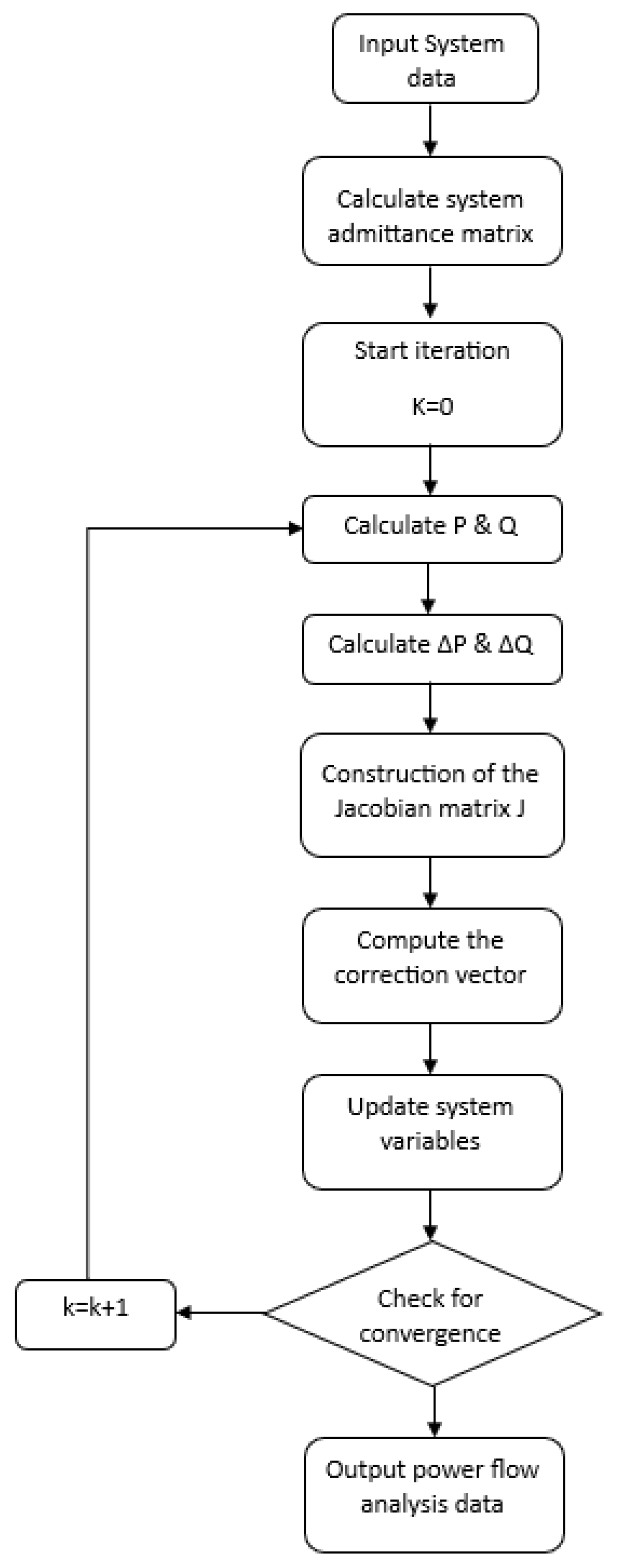
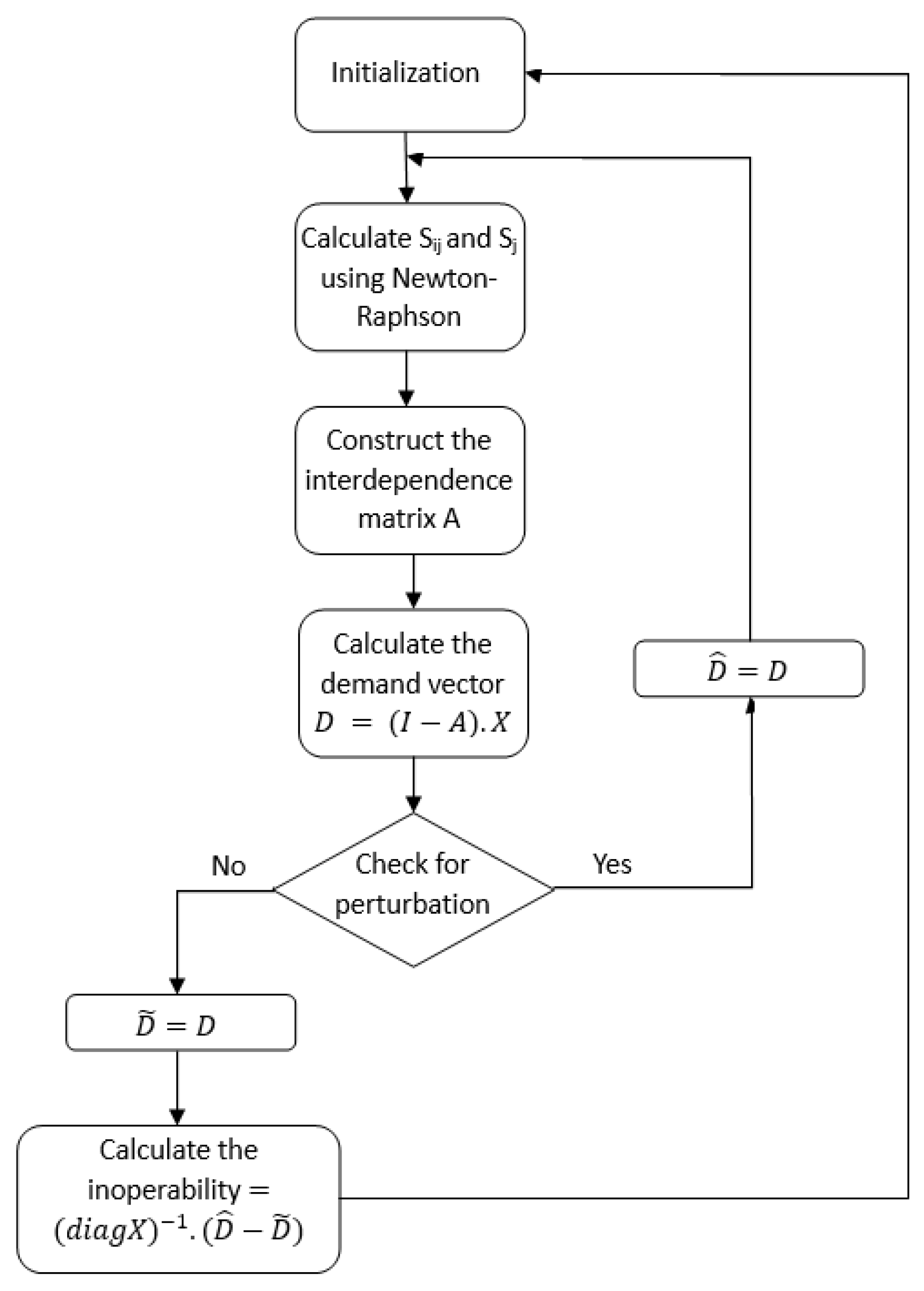
However, the calculation of power transmitted between nodes requires the use of the Newton–Raphson power flow analysis method. This method is employed to determine the steady-state operating conditions of the power grid, encompassing voltages, currents, and power flow through transmission lines and other network elements.

The summarized methodology of the Newton–Raphson power flow analysis is illustrated in the flow chart presented in Figure 3. The initial step involves calculating the admittance matrix based on the power grid lines’ data, incorporating resistance, reactance, and ground admittance.

The bus admittance matrix can be constructed using the following equations:

$${\mathit{z}}_{\mathit{i}}={\mathit{r}}_{\mathit{i}}+\mathit{i}{\mathit{x}}_{\mathit{i}}$$

(7)

$${\mathit{y}}_{\mathit{i}}=\frac{1}{{\mathit{z}}_{\mathit{i}}}$$

(8)

$${\mathit{b}}_{\mathit{i}}=\mathit{i}.{\mathit{b}}_{\mathit{i}}$$

(9)

$${\mathit{Y}}_{\mathit{i}\mathit{i}}={\sum }_{\begin{array}{c}\mathit{j}=0\\ \mathit{j}\ne \mathit{i}\end{array}}^{\mathit{N}}{\mathit{y}}_{\mathit{j}}+{\mathit{b}}_{\mathit{j}}$$

(10)

$${\mathit{Y}}_{\mathit{i}\mathit{j}}=-{\mathit{y}}_{\mathit{j}}$$

(11)

where:

r: Bus resistance in per unit

x: Bus reactance in per unit

b: Bus ground admittance in per unit

y: Admittance

z: Impedance

Hence, the impedance matrix can be calculated using the following equation:

$${\mathit{Y}}_{\mathit{b}\mathit{u}\mathit{s}}^{-1}={\mathit{Z}}_{\mathit{b}\mathit{u}\mathit{s}}$$

(12)

The second step is to calculate the active and reactive power at each bus using the following equations:

$${\mathit{P}}_{\mathit{i}}={\mathit{V}}_{\mathit{i}}{\sum }_{\mathit{j}=1}^{\mathit{N}}\left|{\mathit{V}}_{\mathit{i}}\right|\left|{\mathit{V}}_{\mathit{j}}\right|\left({\mathit{G}}_{\mathit{i}\mathit{j}}\mathbf{cos}{\mathit{\theta }}_{\mathit{i}\mathit{j}}+{\mathit{B}}_{\mathit{i}\mathit{j}}\mathbf{sin}{\mathit{\theta }}_{\mathit{i}\mathit{j}}\right)$$

(13)

$${\mathit{Q}}_{\mathit{i}}={\mathit{V}}_{\mathit{i}}{\sum }_{\mathit{j}=1}^{\mathit{N}}\left|{\mathit{V}}_{\mathit{i}}\right|\left|{\mathit{V}}_{\mathit{j}}\right|\left({\mathit{G}}_{\mathit{i}\mathit{j}}\mathbf{sin}{\mathit{\theta }}_{\mathit{ij}}-{\mathit{B}}_{\mathit{i}\mathit{j}}\mathbf{cos}{\mathit{\theta }}_{\mathit{i}\mathit{j}}\right)$$

(14)

where ${\mathit{G}}_{\mathit{i}\mathit{j}}$ and ${\mathit{B}}_{\mathit{i}\mathit{j}}$ are, respectively, the real and imaginary parts of the admittance between the buses i and j.

The Newton–Raphson method compares the calculated power injections with the specified or desired ones at each bus. The ΔP and ΔQ values denote the mismatches between the specified and calculated power injections at each bus in the system. The Newton–Raphson algorithm utilizes these mismatches to iteratively update voltage magnitudes and phase angles until the mismatches converge to acceptable levels, signifying satisfaction of the power flow equations. The iterative process includes adjusting voltage magnitudes and phase angles using the calculated ΔP and ΔQ values to enhance the accuracy of the power flow solution until convergence is attained.

The Newton–Raphson method applied to power flow can be summarized as follows:

$$\left[\begin{array}{c}∆{\mathit{P}}_2\\ ⋮\\ \begin{array}{c}∆{\mathit{P}}_{\mathit{N}}\\ ∆{\mathit{Q}}_2\\ \begin{array}{c}⋮\\ ∆{\mathit{Q}}_{{\mathit{N}}^{\prime }}\end{array}\end{array}\end{array}\right]=\mathit{J}\times \left[\begin{array}{c}∆{\mathit{\delta }}_2\\ ⋮\\ \begin{array}{c}∆{\mathit{\delta }}_{\mathit{N}}\\ ∆{|\mathit{V}}_2|\\ \begin{array}{c}⋮\\ ∆{|\mathit{V}}_{{\mathit{N}}^{\prime }}|\end{array}\end{array}\end{array}\right]$$

(15)

where J is the Jacobian square matrix: $\mathit{J}=\left[\begin{array}{cc}{\mathit{J}}_1& {\mathit{J}}_2\\ {\mathit{J}}_3& {\mathit{J}}_4\end{array}\right]$

$${\mathit{J}}_1=\frac{\partial {\mathit{P}}_{\mathit{i}}}{\partial {\mathit{\delta }}_{\mathit{j}}}{;\mathit{J}}_2=\frac{\partial {\mathit{P}}_{\mathit{i}}}{\partial \left|{\mathit{V}}_{\mathit{j}}\right|}{;\mathit{J}}_3=\frac{\partial {\mathit{Q}}_{\mathit{i}}}{\partial {\mathit{\delta }}_{\mathit{j}}}{;\mathit{J}}_4=\frac{\partial {\mathit{Q}}_{\mathit{i}}}{\partial \left|{\mathit{V}}_{\mathit{j}}\right|}$$

(16)

$$\frac{\partial {\mathit{P}}_{\mathit{i}}}{\partial {\mathit{\delta }}_{\mathit{i}}}={\sum }_{\mathit{j}\ne \mathit{i}}\left|{\mathit{V}}_{\mathit{i}}\right|\left|{\mathit{V}}_{\mathit{j}}\right|\left|{\mathit{Y}}_{\mathit{i}\mathit{j}}\right|\mathbf{sin}\left({\mathit{\theta }}_{\mathit{i}\mathit{j}}-{\mathit{\delta }}_{\mathit{i}}+{\mathit{\delta }}_{\mathit{j}}\right)$$

(17)

$$\frac{\partial {\mathit{P}}_{\mathit{i}}}{\partial {\mathit{\delta }}_{\mathit{j}}}=-\left|{\mathit{V}}_{\mathit{i}}\right|\left|{\mathit{V}}_{\mathit{j}}\right|\left|{\mathit{Y}}_{\mathit{i}\mathit{j}}\right|\mathbf{sin}\left({\mathit{\theta }}_{\mathit{i}\mathit{j}}-{\mathit{\delta }}_{\mathit{i}}+{\mathit{\delta }}_{\mathit{j}}\right);\mathit{j}\ne \mathit{i}$$

(18)

$$\frac{\partial {\mathit{P}}_{\mathit{i}}}{\partial {|\mathit{V}}_{\mathit{i}}|}=2\left|{\mathit{V}}_{\mathit{i}}\right|\left|{\mathit{Y}}_{\mathit{i}\mathit{j}}\right|\mathbf{cos}{\mathit{\theta }}_{\mathit{i}\mathit{i}}+{\sum }_{\mathit{j}\ne \mathit{i}}\left|{\mathit{V}}_{\mathit{j}}\right|\left|{\mathit{Y}}_{\mathit{i}\mathit{j}}\right|\mathbf{cos}\left({\mathit{\theta }}_{\mathit{i}\mathit{j}}-{\mathit{\delta }}_{\mathit{i}}+{\mathit{\delta }}_{\mathit{j}}\right)$$

(19)

$$\frac{\partial {\mathit{P}}_{\mathit{i}}}{\partial {|\mathit{V}}_{\mathit{j}}|}=\left|{\mathit{V}}_{\mathit{i}}\right|\left|{\mathit{Y}}_{\mathit{i}\mathit{j}}\right|\mathbf{cos}\left({\mathit{\theta }}_{\mathit{i}\mathit{j}}-{\mathit{\delta }}_{\mathit{i}}+{\mathit{\delta }}_{\mathit{j}}\right);\mathit{j}\ne \mathit{i}$$

(20)

$$\frac{\partial {\mathit{Q}}_{\mathit{i}}}{\partial {\mathit{\delta }}_{\mathit{i}}}={\sum }_{\mathit{j}\ne \mathit{i}}\left|{\mathit{V}}_{\mathit{i}}\right|\left|{\mathit{V}}_{\mathit{j}}\right|\left|{\mathit{Y}}_{\mathit{i}\mathit{j}}\right|\mathbf{cos}\left({\mathit{\theta }}_{\mathit{i}\mathit{j}}-{\mathit{\delta }}_{\mathit{i}}+{\mathit{\delta }}_{\mathit{j}}\right)$$

(21)

$$\frac{\partial {\mathit{Q}}_{\mathit{i}}}{\partial {\mathit{\delta }}_{\mathit{j}}}=-\left|{\mathit{V}}_{\mathit{i}}\right|\left|{\mathit{V}}_{\mathit{j}}\right|\left|{\mathit{Y}}_{\mathit{i}\mathit{j}}\right|\mathbf{cos}\left({\mathit{\theta }}_{\mathit{i}\mathit{j}}-{\mathit{\delta }}_{\mathit{i}}+{\mathit{\delta }}_{\mathit{j}}\right);\mathit{j}\ne \mathit{i}$$

(22)

$$\frac{\partial {\mathit{Q}}_{\mathit{i}}}{\partial {|\mathit{V}}_{\mathit{i}}|}=-2\left|{\mathit{V}}_{\mathit{i}}\right|\left|{\mathit{Y}}_{\mathit{i}\mathit{j}}\right|\mathbf{sin}{\mathit{\theta }}_{\mathit{i}\mathit{i}}-{\sum }_{\mathit{j}\ne \mathit{i}}\left|{\mathit{V}}_{\mathit{j}}\right|\left|{\mathit{Y}}_{\mathit{i}\mathit{j}}\right|\mathbf{sin}\left({\mathit{\theta }}_{\mathit{i}\mathit{j}}-{\mathit{\delta }}_{\mathit{i}}+{\mathit{\delta }}_{\mathit{j}}\right)$$

(23)

$$\frac{\partial {\mathit{Q}}_{\mathit{i}}}{\partial {|\mathit{V}}_{\mathit{j}}|}=-\left|{\mathit{V}}_{\mathit{i}}\right|\left|{\mathit{Y}}_{\mathit{i}\mathit{j}}\right|\mathbf{sin}\left({\mathit{\theta }}_{\mathit{i}\mathit{j}}-{\mathit{\delta }}_{\mathit{i}}+{\mathit{\delta }}_{\mathit{j}}\right);\mathit{j}\ne \mathit{i}$$

(24)

where:

θ: Bus voltage phase angle (rad)

V: Bus voltage magnitude (V)

P: Active power (MW)

Q: Reactive power (MVAr)

Δ: Phase shift angle (rad)

In the final step of the Newton–Raphson power flow iteration, the correction vector is computed to update the system variables. This correction vector represents the adjustments made to the voltage magnitudes and phase angle estimates at each iteration of the algorithm. It plays a crucial role in iteratively refining the solutions until the power flow equations converge to a stable solution.

The correction vector, denoted as ∆X, encompasses changes in voltage magnitudes and phase angles at each bus within the power system. It is computed using the Jacobian matrix and the power mismatch vectors (ΔP and ΔQ) at each iteration. The general form of the correction vector in the Newton–Raphson method can be expressed as:

$$∆\mathit{X}={\mathit{J}}^{-1}\left[\begin{array}{c}∆\mathit{P}\\ ∆\mathit{Q}\end{array}\right]$$

The Jacobian matrix, denoted as J, quantifies the sensitivity of power mismatches (ΔP and ΔQ) to voltage magnitudes and phase angle changes. It is computed using partial derivatives of power flow equations concerning voltage magnitudes and angles. Meanwhile, the correction vector ΔX, obtained by multiplying the inverse Jacobian matrix with the power mismatch vectors, facilitates necessary adjustments to update the voltage magnitudes and phase angle estimates at each bus. These updates enhance the accuracy of power flow solutions in subsequent iterations of the Newton–Raphson algorithm.

The iterative application of the correction vector to update the voltage magnitudes and phase angle estimates continues until the changes in these quantities reach sufficiently small values, indicating convergence to a solution where the power flow equations are satisfied within acceptable tolerances.

5. Simulation Model and Results Analysis

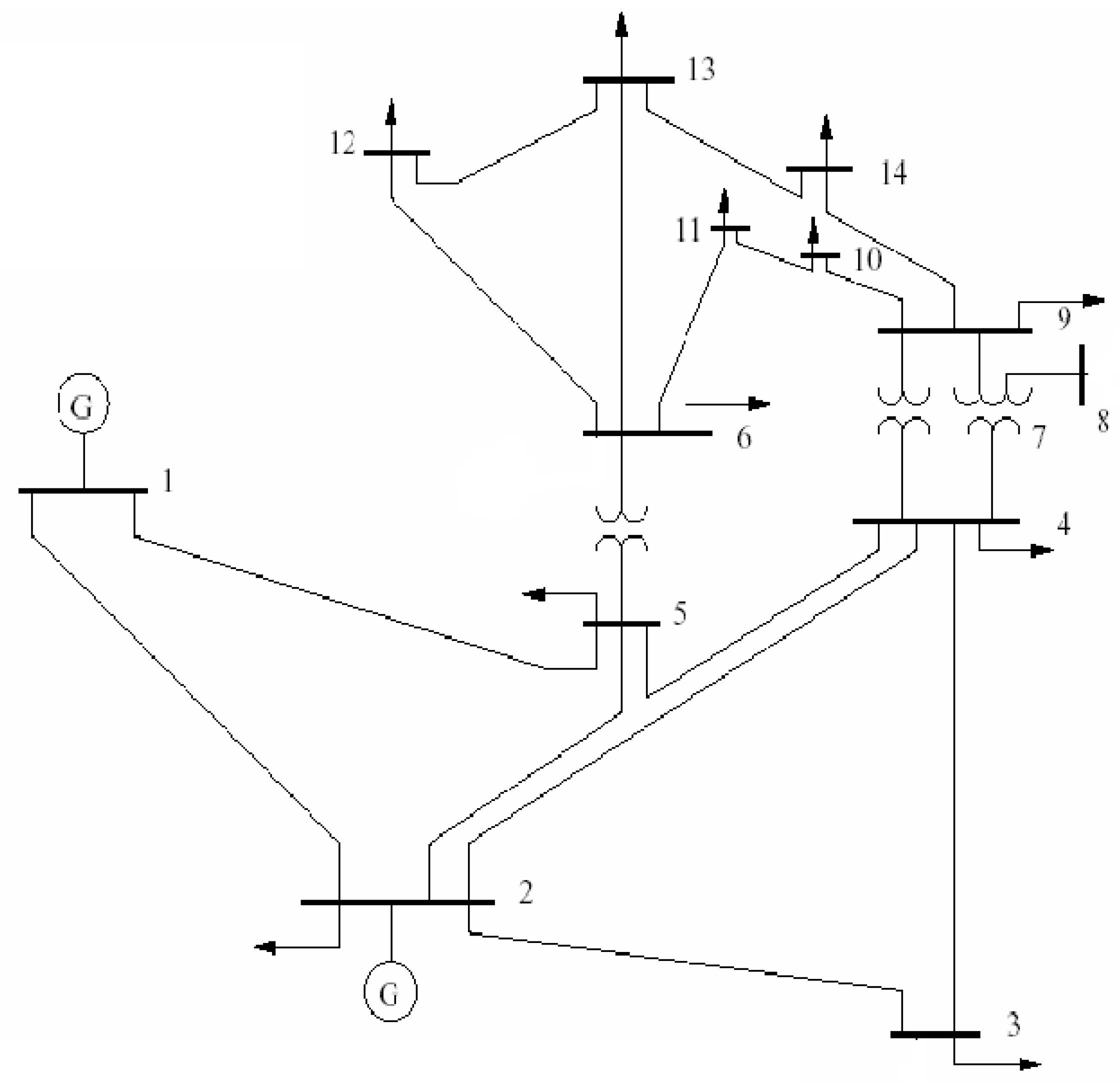
To assess the resilience of centralized versus decentralized electric grids, the IEEE-14 node power grid system was selected as the baseline model (Figure 4). The standard IEEE-14 node power system represents the centralized electric grid (Model A). Grid data details are provided in Appendix A.

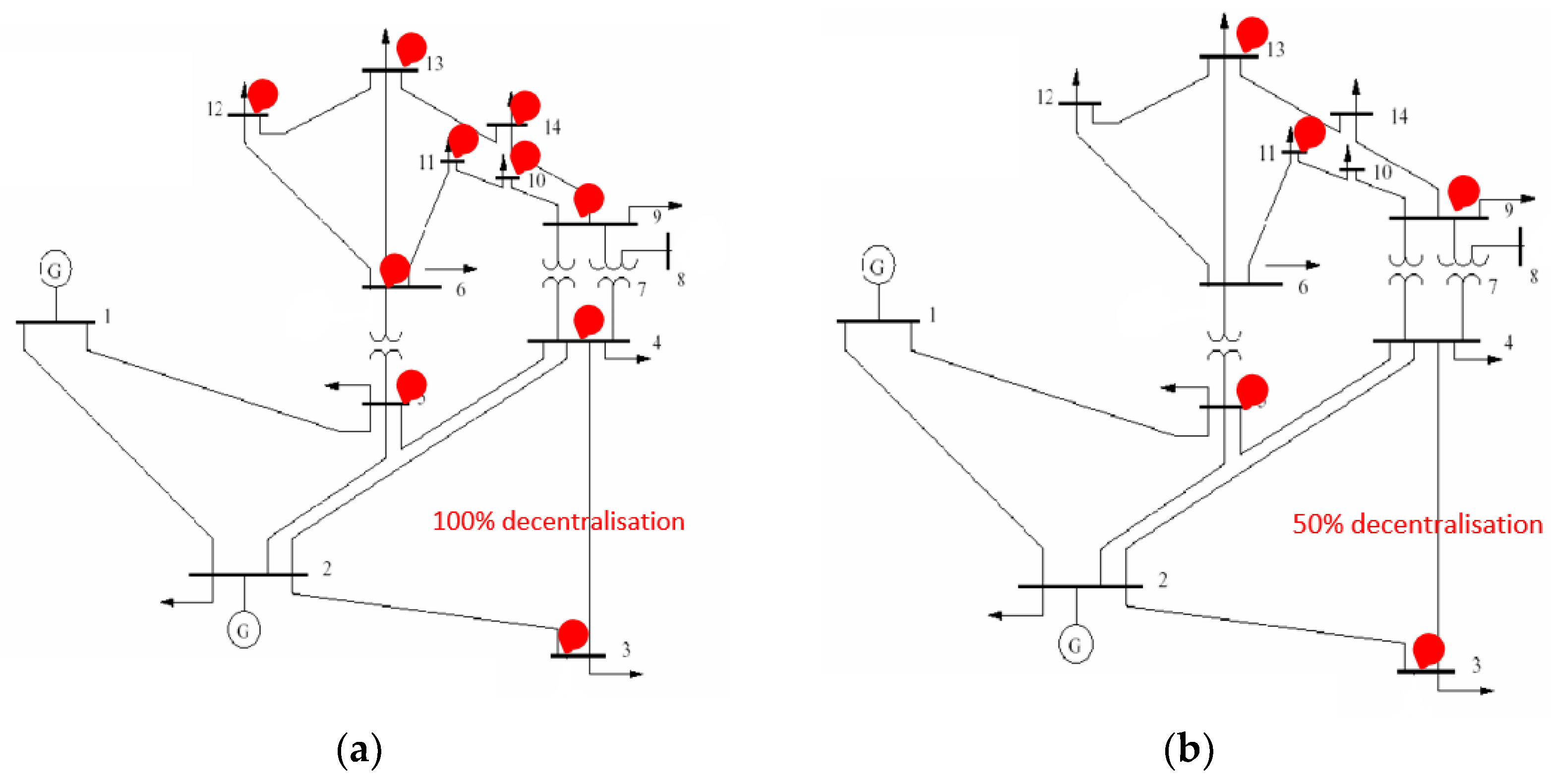
Two modified IEEE-14 node power system models were employed for comparative analysis to represent decentralized electric grids. The first model, illustrated in Figure 5a, integrates a distributed energy resource of 10 MW connected to buses 3, 4, 5, 6, 9, 10, 11, 12, 13, and 14, categorizing it as the 100% decentralized model (Model B). The second model, depicted in Figure 5b, features a distributed energy resource of 10 MW connected to buses 3, 5, 9, 11, and 13, representing the 50% decentralized electric grid (Model C).

The perturbation simulation involved two scenarios. In the first scenario, a fault disconnected generator #2 from bus #2 and interrupted the transmission line between bus #2 and bus #5. Scenario #1 is depicted in Figure 6a. The second scenario extended the faults in scenario #1, introducing an additional interruption in the transmission line and substation connecting bus #4 to bus #9. Scenario #2’s faults are illustrated in Figure 6b.

The experiment utilized an Intel i7-7500U, 2.70 GHz, dual-core CPU with 16 GB RAM, operating on Windows 120. The algorithms were implemented in MATLAB R2022a (codes provided in Appendix B and Appendix C). The outcomes were validated against results obtained by simulating the same models under the same scenarios using the Electrical Transient Analyzer Program version 12.6.0 (ETAP), a software platform used to design, simulate, analyze, control, optimize, and automate electrical power systems. Both models gave practically the same results.

The simulation flowchart for comparing the centralized vs. decentralized electric grid is presented in Figure 7. This simulation employs the calculated inoperability value to assess the resilience of each electric grid model when facing similar interruptions. At time t = 0, the electric grid is considered undisturbed. The faults of scenario #1 are applied to each of the three grid models, and the inoperability of each bus is computed. Subsequently, the conditions of scenario #2 are uniformly applied to all three models, and new inoperability values are determined. By computing the inoperability value for each bus of each model using the IIM, we can compare the resilience of the centralized and decentralized grids under identical conditions.

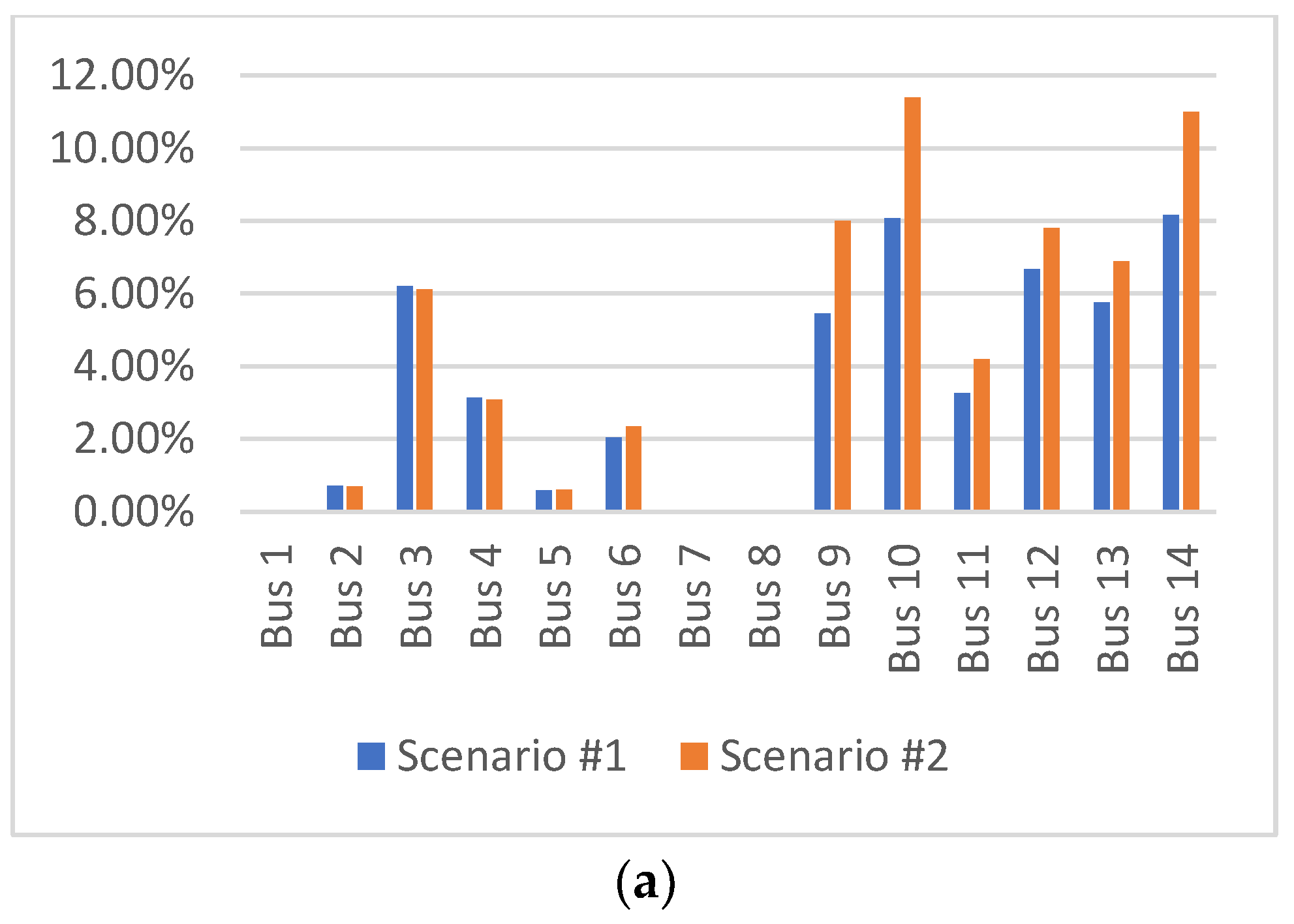
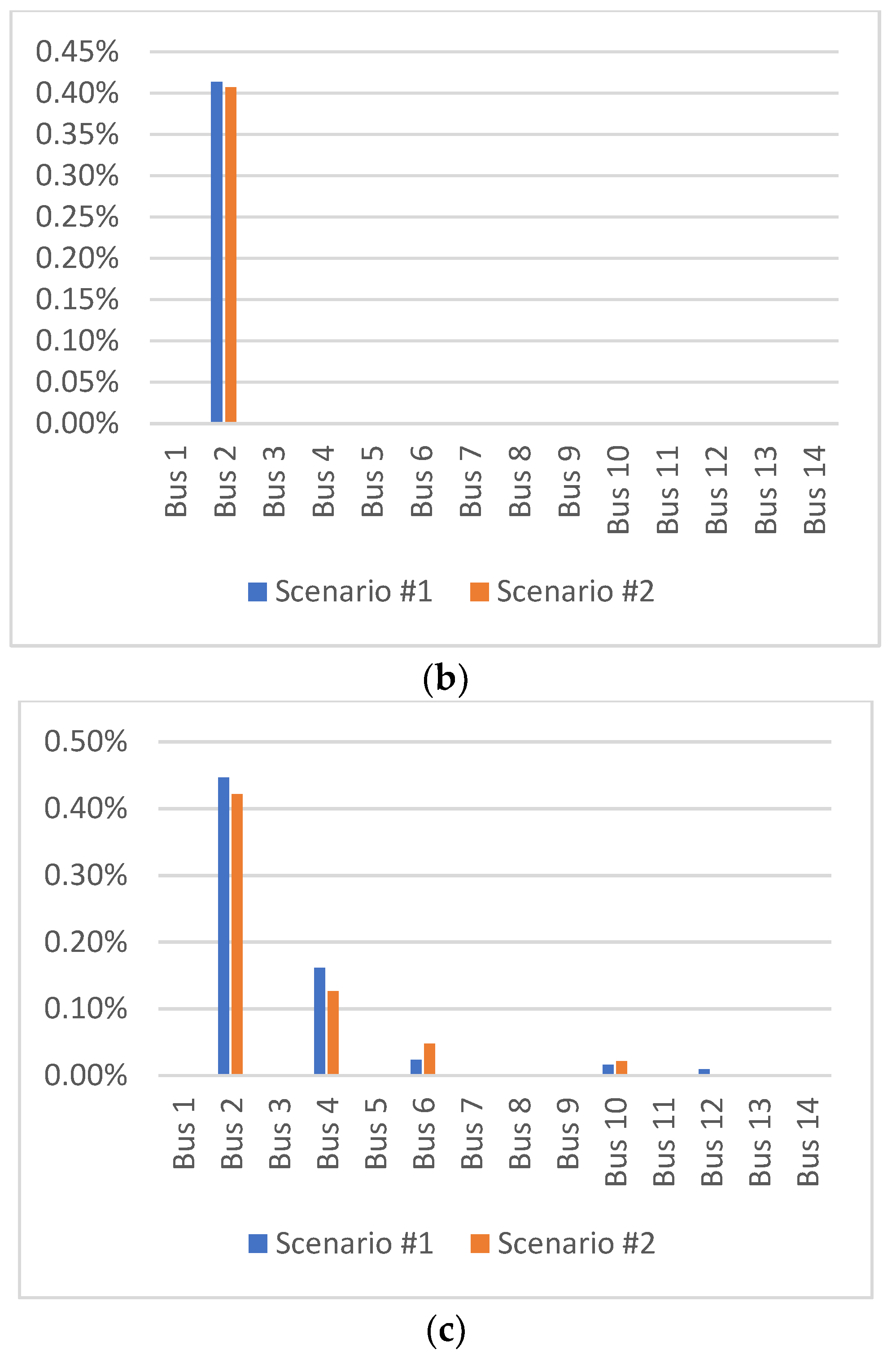
The simulation results are depicted in Figure 8. As no load is connected to buses 1, 7, and 8, and considering the inoperability definition provided in Equation (6), zero inoperability is expected for these three buses, regardless of any interruption or disturbance to the grid.

The results depicted in Figure 8a clearly show that disturbances caused by scenarios #1 and #2 affected all buses except buses 1, 7, and 8, as explained earlier. The inoperability values resulting from the simulation of model A (centralized electric grid) demonstrate that in a centralized system, a perturbation or interruption on a single line or bus affects the entire grid, particularly the remote nodes such as buses 9, 10, 11, 12, 13, and 14. This contrasts with decentralized grids. The inoperability values of model B (fully decentralized model) indicate that only bus 2 was affected by the perturbations of scenario #1, mainly due to the disconnection of generator 2 supplying this bus. Additionally, the disconnection of buses 5–9 had minimal impact on the grid because the DERs connected to the buses had enough power to meet the demand. On the other hand, the simulation results of model C (partially decentralized model) show that several buses were affected by the interruptions, specifically the buses where no DERs are connected (buses 2, 4, 6, 10, and 12), highlighting the importance of connecting DERs to all nodes to increase the grid’s flexibility, reduce technical losses, and enhance its resilience and reliability.

Notably, the intolerabilities calculated in models B and C are considerably lower than the results obtained with model A. The intolerabilities in model A ranged between 0.6% and 11.4%. However, with models B and C, these values did not exceed 0.45%. This emphasizes that decentralization affects the number of nodes impacted by a disturbance or interruption and reduces the magnitude of this interruption on the affected buses.

6. Conclusions

The future of grid resilience lies in balancing centralized and decentralized approaches. While centralized grids have been effective in the past, the demand for greater energy resilience, sustainability, and adaptability necessitates a shift towards decentralized grids. The findings of this study demonstrate that decentralized systems provide improved resilience through increased flexibility and modularity. Moreover, it proves that decentralization, through dispersing generation and storage assets across the grid, minimizes the impact of individual failures and makes the system more resilient to disruptions. In the event of a disruption or failure at one location, other distributed resources can continue to supply power, reducing the risk of widespread outages and enhancing overall system robustness. The results obtained in our simulation show that a completely decentralized electric grid is, to a certain extent, immune to interruptions caused by extreme weather events, natural disasters, and other emergencies that can disrupt conventional centralized infrastructure.

However, collaboration among policymakers, grid operators, utilities, and communities is essential in order to transition to decentralized grids successfully. Investments in research and development, infrastructure upgrades, and regulatory frameworks should be coordinated to support the growth of decentralized grids. Furthermore, while decentralized grids hold significant promise, notable challenges must be addressed. One major hurdle is the cost of implementing decentralized systems and upgrading existing infrastructure. The initial investments for distributed generation, energy storage, and grid interconnections can be considerable. However, with the ongoing decline in the costs of renewable energy technologies and storage systems, the economic feasibility of decentralized grids is improving. Another challenge lies in integrating decentralized systems into existing regulatory frameworks and grid management practices. Shifting from a centralized to a decentralized model necessitates the development of new policies and regulations that facilitate the deployment and operation of distributed energy resources. Grid operators and utilities must adapt their planning and operational models to accommodate the dynamic nature of decentralized grids, ensuring grid stability and reliability.

Despite these challenges, the opportunities presented by decentralized grids are substantial. They offer the potential for increased energy independence, reduced reliance on fossil fuels, and the integration of innovative technologies and business models. Decentralized grids empower communities and individuals to participate actively in the energy transition, fostering a sense of ownership and resilience at the local level.

Moreover, the modern electric grid comprises three physical, communication, and data management layers. While decentralization has enhanced the resilience of the physical layer, the other two layers remain vulnerable. Many electric grids, even those with significant integration of distributed energy resources, still depend on a centralized control center, acting as an SPOF. Consequently, there is a growing need to decentralize all three layers of the electric grid to achieve a higher level of resilience. Additionally, as the electric grid undergoes a rapid digital transformation, the securitization of data and digital processes lags behind. Addressing this discrepancy is crucial to ensure the comprehensive resilience of the electric grid in the face of evolving technological challenges.

This study provides concrete evidence of the positive impact of physical decentralization on electric grid resilience. It also highlights a broader topic that warrants further investigation in the ongoing pursuit of achieving an elevated level of electric grid reliability. The findings underscore the importance of considering both physical and digital decentralization to enhance the resilience of modern energy infrastructure comprehensively. On another level, this article offers a new mathematical simulation based on Leontief’s IO model to assess and analyze the resilience of the electric grid. The proposed model does not require considerable computational resources and requires minimal simulation time, making it easy to code into a simple tool and use as simulation software.