Article

Global Methods for Calculating Shading and Blocking Efficiency in Central Receiver Systems

1
E.T.S. Ingeniería, Universidad de Huelva (UHU), Campus El Carmen, Avd. Tres de Marzo, s/n, 21071 Huelva, Spain
2
E.T.S. Ingenieros Industriales, Universidad Nacional de Educación a Distancia (UNED), C/Juan del Rosal, 12, 28040 Madrid, Spain
*
Author to whom correspondence should be addressed.
Energies 2024, 17(6), 1282; https://doi.org/10.3390/en17061282
Submission received: 25 January 2024 / Revised: 28 February 2024 / Accepted: 5 March 2024 / Published: 7 March 2024
(This article belongs to the Special Issue Concentrating Solar Power Plants)

Abstract

:
This paper presents three new methods for calculating the shading and blocking efficiency in Central Receiver Systems (CRSs). All of them are characterized by the calculation of multiple useful and total reflecting areas without the need to resort to parallel calculation in the CPU or GPU, and by low computation times and minimum errors. They are being specially designed for implementation in codes focused on heliostat field design and optimization in CRSs. The proposed methods have been compared against two outstanding “individual” methods (homology and Boolean operations), in addition to a reference case based on the Monte Carlo ray-tracing (MCRT) technique. The results indicate that one of the proposed methods presents reduced error values and high computational speed, even relaxing the restrictions on candidate filtering. At the same error level, the global method is up to 7.80 times faster than the fastest individual method (homology) and up to 194 times faster than the method based on the MCRT technique. The causes of the main errors of each method are also analyzed.

1. Introduction

Central Receiver Systems (CRSs) have become an integral part of Concentrated Solar Power (CSP) technology, an approach that has been demonstrated in commercial-scale projects worldwide and received substantial study and experimentation in the past decades. However, there are still areas where further research and development are needed to improve the efficiency and cost-effectiveness of the technology.
An important factor in the overall efficiency of a CRS is the optics of the heliostats. Shading and blocking in a heliostat field are particularly significant issues, as they can reduce the solar power that is reflected onto the receiver, and thus decrease the overall efficiency of the system.
The shading and blocking efficiency of a heliostat can be calculated as the ratio of useful to total reflecting area. The value depends on the relative position and orientation of neighboring heliostats.
According to [1,2], the computation codes used in the design of CRSs can be classified into two groups: on the one hand, those applications focused on the detailed simulation of a solar field at a given sample point, and on the other, those focused on calculating the optimal layout, i.e., the most appropriate positions of the heliostats to maximize the annual performance of the plant, or to minimize the cost of the energy produced.
The codes in the first group, such as TONATIUH [3], SolTRACE [4], MIRVAL [5], or STRAL [6], among others, usually consist of MCRT tools aimed at accurately reproducing the geometry of the heliostats, along with the phenomenon of incidence and reflection of the solar radiation, with few simplifications. This means they are able to determine the shading and blocking in the solar field with great accuracy, although the high computation times make them generally unaffordable for optimization purposes. Despite that, in recent years MCRT tools have been developed, such as QMCRT [7] and sbpRAY [8], which, thanks to GPU technology, allow significantly shorter computation times. In this way, these codes can be used both for detailed simulation and optimization purposes.
On the other hand, the codes in the second group introduce some simplifications. Specifically, in order to determine the shading and blocking efficiency, they employ methods based on projection to calculate the useful and total reflecting areas, and they usually establish a limit for the number of shading/blocking candidates per each heliostat analysis. In Table 1, a summary of the initial hypotheses on which the methods based on projection are based is shown.
In accordance with the hypotheses indicated in Table 1, several approaches can be distinguished. The simplest approach adopts hypotheses (i) to (iv) in combination with the use of an oblique cylindrical projection. (According to the direction defined by the solar vector (for shading) and its specular reflection in the center of the heliostat (for blocking), and taking the plane defined by the heliostat under consideration as the projection plane). As a result, the determination of the useful reflecting area is notably simplified. Three groups of codes taking this approach can be distinguished in the literature:
  • Algorithms based on Boolean operations [9,10,11]. They usually follow a multiple-event approach, processing multiple shading/blocking candidates one by one for each considered heliostat. The RCELL code in the UHC suite [12,13] uses a single-event version of these processors. In this case, and like other convolution-based codes (CONCEN [14], DELSOL (Windelsol) [15], and SolarPilot [16]), RCELL employs the cell concept, so shading and blocking calculations are performed on a representative heliostat of the cell to which it belongs.
  • Algorithms based on discretizing the heliostat surface with a uniform mesh, like CONCEN [14] and HLFD [17,18,19,20], all using a multiple-event approach. In this case, if the centers of the grids fall within the projection of a neighboring heliostat, the grids are considered shaded or blocked. Again, this process is carried out candidate by candidate.
  • Algorithms based on discretizing the heliostat surface with uniform vertical stripes. In these codes, the maximum overlapping value is calculated. The most noticeable among this group is the methodology proposed by [21], which has been adopted by other authors, such as Campo [22,23] and [24,25,26,27]. Again, all these methods take a multiple-event approach.
Lipps [11] pointed out that the dominant error affecting all these methodologies comes from hypothesis (iv), leading to a maximum error of approximately 7% at the Barstow pilot plant. Other researchers [28,29,30] have also reported errors due to hypothesis (iv). Furthermore, the use of an oblique cylindrical projection for blocking implies a second source of inaccuracies.
Other authors, such as Raj and Bhattacharya [31], Belaid et al. [32], and Zhang et al. [33], remove hypothesis (iv) and consider instead the orientations of the heliostats with hypotheses (i) to (iii), increasing their accuracy. However, like the methods using hypothesis (iv), they consider all rays reflected as parallel to the specular reflection of the solar vector at its center, which can lead to inaccuracies. In addition, the method proposed by [33] has the drawback of following a single-event approach, so it can only accurately process one candidate per heliostat.
Some efforts have been made to reduce these inaccuracies. Examples include HELIOS [34], homology [35], and simplified ray-tracing [29], as well as the approaches described in [35,36,37], which are based on Boolean operations. All of these incorporate hypotheses (i), (ii), (iii), and (v). Among them, only HELIOS uses a single-event approach, thus limiting its capacity to calculate the overlapping area [38].
Other methods, such as simplified ray-tracing and contour deployment [35], consider only hypotheses (ii), (iii), and (v), and are based on a multiple-event approach in which the heliostats and the candidates are processed one by one.
The method proposed in [39] employs a mixed methodology. The shading calculation is in line with [14] but considers the different orientations of all the neighboring heliostats, assuming hypotheses (i), (ii), and (iii). The blocking calculation uses ray-tracing techniques, assuming hypotheses (ii) and (iii).
Finally, a group of algorithms considers only hypotheses (ii) and (iii), such as the central solar ray-tracing method proposed in [28], the most accurate method of all the above, although at the cost of longer execution times.
This paper presents three new methods based on projection for calculating CRS shading and blocking efficiency. They calculate the useful and total reflecting areas using a novel multiple or global approach, allowing dozens of heliostats to be simultaneously processed (unlike the methods reviewed above) with no need for parallel calculations on a CPU or GPU. All of them dispense with assumption (iv), take a multiple-event approach, and have a “robust” algorithm capable of processing heliostat fields of diverse configurations and geometries. In addition to that, they allow for a basic filtering of candidates without losing accuracy.
This set of features can be advantageous for design and optimization purposes, where the appropriate methodology must combine low computation times and reduced deviations. To evaluate these aspects, the presented methods are compared with two “individual” methods, and another method based on the MCRT technique, which is used as a reference case. All of them were implemented in Matlab® R2022a.
In the following sections, first, the procedure for projecting the heliostats in the solar field for a given sample point is explained. Then, the three proposed global methods are described. Finally, a comparison of the deviations and computation times is carried out, using as a reference case the results obtained by a method based on the MCRT technique.

2. Methodology

This section presents three new global methods for calculating the shading and blocking efficiency:
  • GM1—discretization in elementary rectangles,
  • GM2—numerical integration by vertical stripes, and
  • GM3—the starting point method.
Once these models have been described, their results and performance are compared with two “individual” methods based on the same initial hypotheses—M3, homology, and M4, Boolean operations—proposed and analyzed by [35]. A sixth method M0—based on MCRT [35]—was chosen as a reference case.
Before introducing the methods, the initial hypotheses and the methodology used for heliostat projections are outlined below.

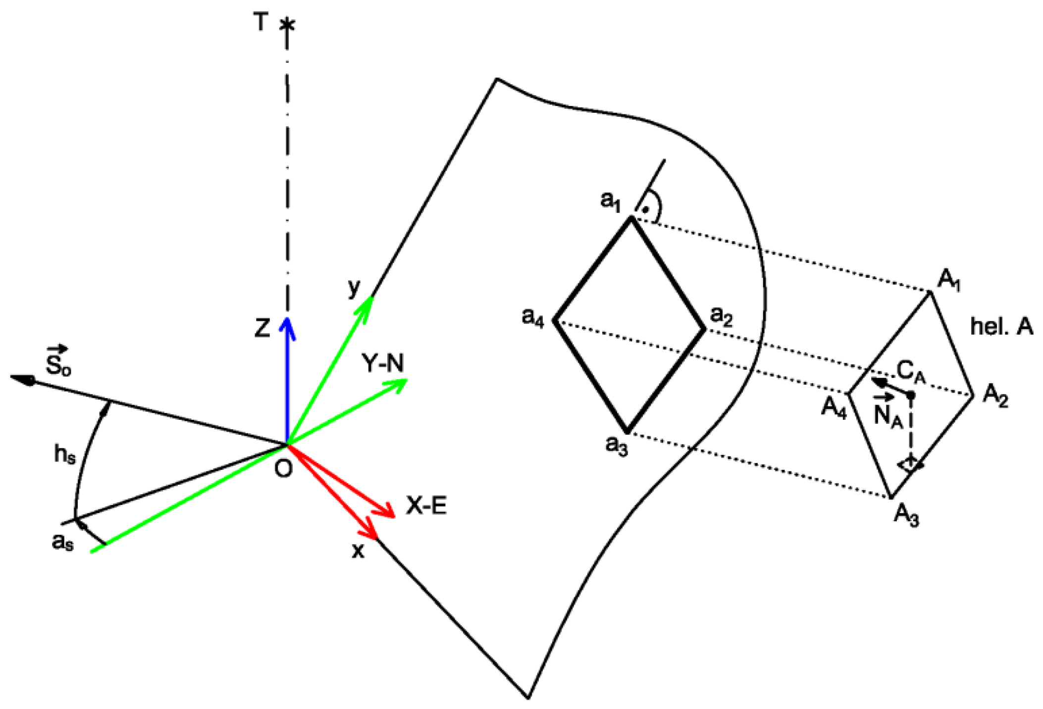
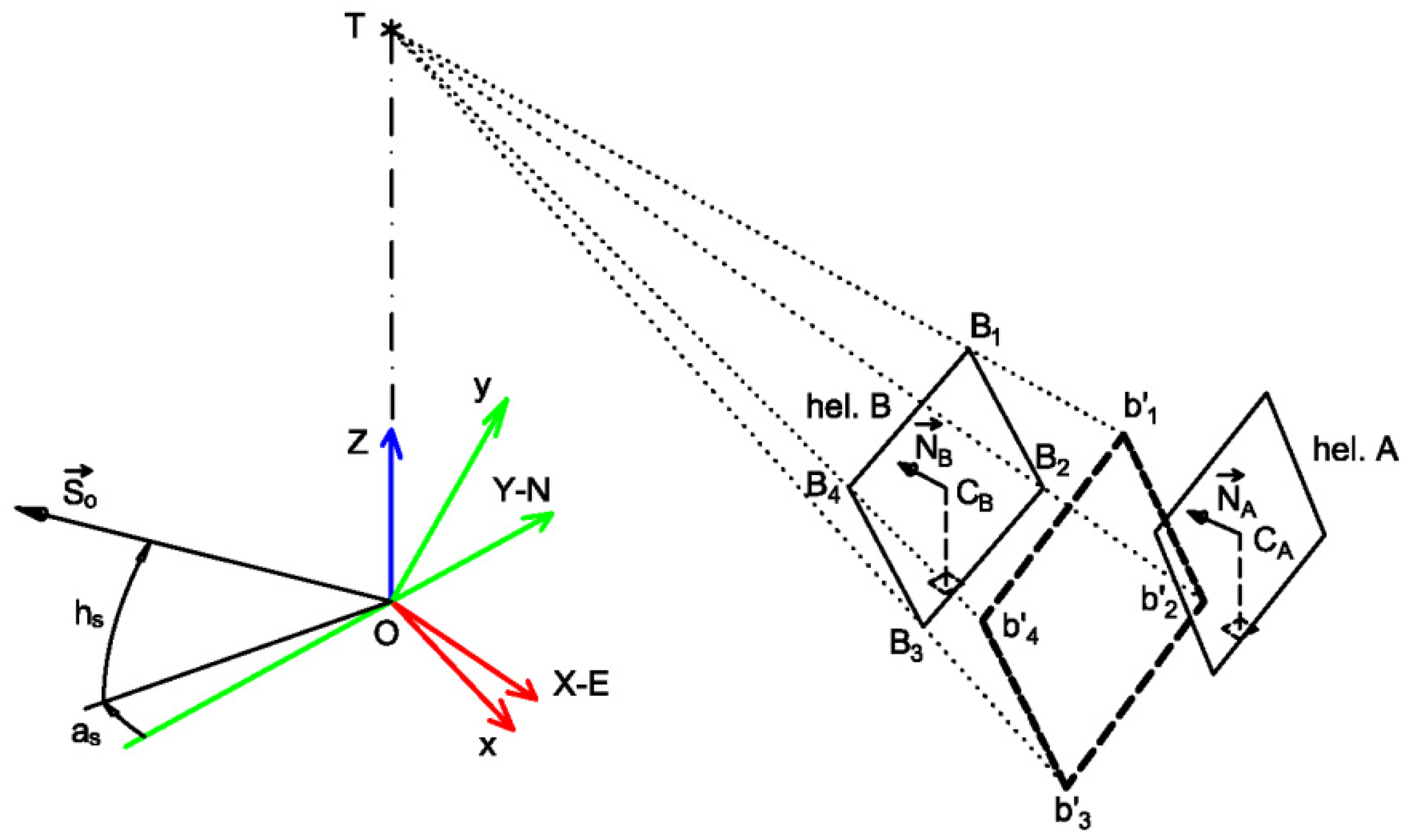
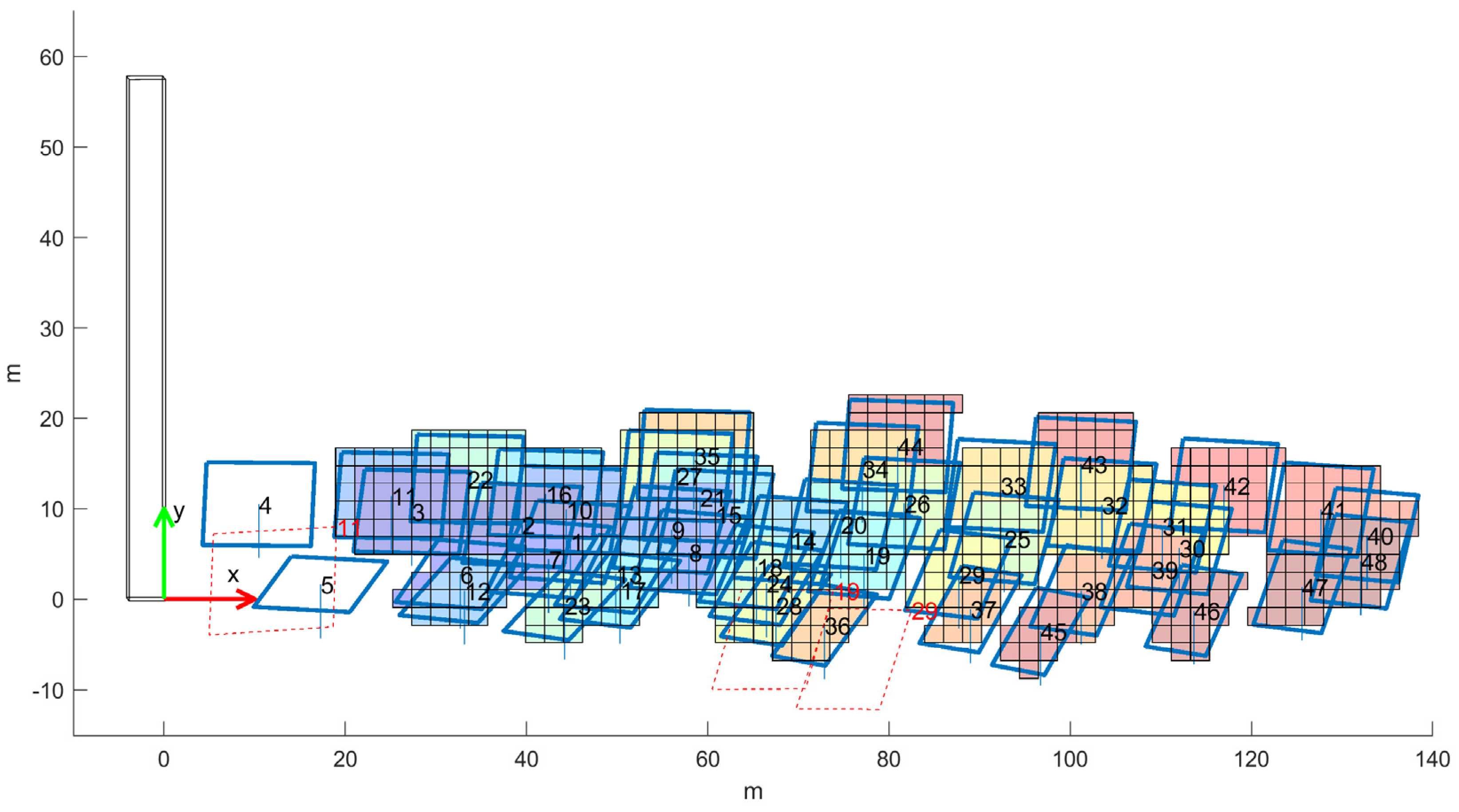
2.1. Initial Hypotheses—Heliostat Projections

The proposed global methods consider the following assumptions:
(i).
The surface of the heliostats is a flat rectangular sheet.
(ii).
The sunshape model is a point source sun.
(iii).
Optical errors are null.
(v).
All rays reflected by a heliostat converge precisely at the center of the target.
Likewise, the following conventions will be used in notation:
  • Capital letters are used to indicate points and lines in space.
  • Lowercase letters are used to indicate projections of points and lines.
The set of assumptions above considers the different orientations of the heliostats. Furthermore, the projection methodology, the candidate pre-selection method [40], and the global methods that will be developed in Section 2.2 are valid under the following assumptions: (1) any heliostat field layout; (2) any latitude north or south; (3) any heliostat sun-tracking; (4) unequal-sized heliostats; (5) centers of the heliostats at different heights.
Once the N heliostats in the field are oriented, they are projected onto an oxy plane perpendicular to So (solar vector) that passes through the origin of the universal coordinate system. Two cases are distinguished:
(1) Projection for the shading calculation (Figure 1): This is obtained by projecting the vertices of the heliostat field onto the oxy plane using orthogonal cylindrical projection, with the projecting lines being parallel to So. The following expression is used for this:
a i = S P 1 · A i
where SP is the change-of-basis matrix from the oxy to the OXYZ coordinate system.
Thus, the first two components of ai define the projection of Ai in the oxy reference system, while the third component of ai plays an important role, as it allows the heliostats in the field to be “ordered by depth”. The projection obtained for any heliostat is, in general, a rhomboid. (Note that when using orthogonal cylindrical projection, the projection of a heliostat A can only be a rectangle if, and only if, So · NA = 1. This circumstance occurs, at most, twice a year, leaving the heliostat A shaded by the tower). The operation described by expression (1) is performed simultaneously for the four vertices of all heliostats to be projected, without the need for an iterative process. Consequently, this sub-process is solved in a computationally efficient manner.
(2) Projection for the blocking calculation: This is obtained by performing two successive projections of the heliostats that produce blocking. (2.1) First, the vertices of the heliostat producing the blocking are projected onto the plane defined by the blocked heliostat using a central projection, the center of projection being the target point T (Figure 2). (2.2) Then, as this projection is analogous to that of the shading calculation, expression (1) can be applied to the vertices bi obtained in step (2.1). The projection obtained for any heliostat is, in general, a trapezoid.
To obtain the central projection, a line-plane intersection algorithm is applied which performs the process simultaneously, projecting all the heliostats producing blocking onto the plane defined by the respective blocked heliostats. This sub-process is therefore computationally efficient. Figure 3 shows the result of the projection process for a small example field, with a radial stagger arrangement of 48 heliostats, in which the heliostats projected by shading and blocking are represented with solid and dashed lines, respectively.
In Figure 3, the notation used for the heliostats projected by blocking (dashed line), for example, 13–24, indicates that heliostat 13 blocks heliostat 24.

2.2. Global Methods

In Section 2.1 we described the mechanism for obtaining the data required for the global methods using a two-dimensional representation. In the GM1 method, the oxy projection plane is divided into uniform horizontal and vertical stripes, while in GM2 and GM3 it is divided into vertical stripes only. All three methods involve iteratively sweeping the projection plane from left to right, calculating the useful and total reflecting area of all intercepted heliostats simultaneously by taking into account shading and blocking (Figure 4). The global methods are not heavily dependent on candidate selection or filtering algorithms and only require basic filtering for blocking, given that when instances occur of the superposition of projected heliostats they assign the useful reflecting area to the highest heliostat (largest z-coordinate at its center). A consequence of this feature is that the computation times can be reduced due to the use of less demanding filtering systems.
All the global methods presented here also support parallel calculation, distributing the iterations of the main loop independently across various CPU cores. Notwithstanding, for the purposes of comparison, all execution times indicated in this paper were obtained with this function disabled. Below, the three global methods are described.

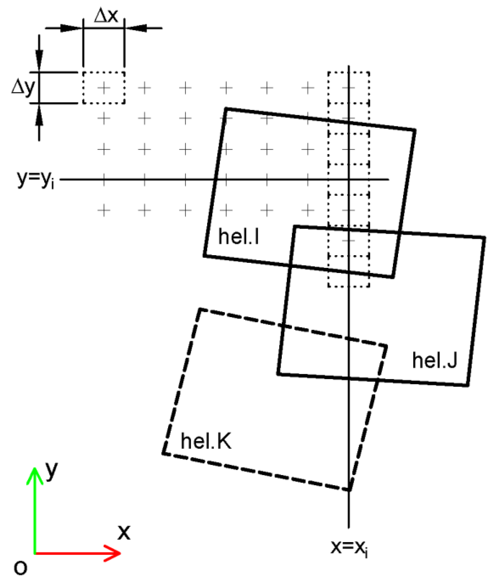
2.2.1. Discretization in Elementary Rectangles (GM1)

The procedure for obtaining the shading and blocking efficiency can be summarized as follows:
  • A mesh of m × n points (xi, yi) is considered on the oxy plane, with uniform separations Δx and Δy along each axis.
  • An iterative process is started that goes through the m values of xi.
2.1. The heliostats cut by the line x = xi are selected. In general, s and b heliostats projected by shading and blocking, respectively (Figure 5).
2.2. The logical matrix A, with n rows and (s + b) columns, is obtained using the following expression:
A = y l T < y 1 : y n y 1 : y n < y u T
where yu and yl denote, respectively, the upper and lower y-coordinate obtained by the intersection of the line x = xi with each of the selected heliostats.
2.3. The overlaps for shading are solved. For this, the following expression is used:
A , 1 : s Z
where row matrix Z, with s columns, contains the z-coordinate of the s heliostats centers; and the operator represents the element-wise product.
Next, the logical matrix B, with n rows and s columns, is derived by setting the cells with maximum values from (3) to “1” and the others to “0”. Each row has, at most, one true value.
This step ensures that, if in the same calculation point (xi, yi) two or more heliostats coexist, the true value corresponds only to the highest of all those that match.
2.4. The overlaps for blocking are solved. For this, the columns r and t are determined in which the blocked heliostat and the one producing the blocking are involved, respectively, and the following expression is applied, which will be repeated b times:
B , r = B , r     ¬ A , t
This step ensures that, if in the same calculation point (xi, yi) the blocked heliostat and the blocking heliostat coexist, the cells overlapped by blocking are noted to be assigned with false values.
2.5. The useful and total reflecting area, in the abscissa x = xi, of an arbitrary heliostat that occupies column r can be calculated, respectively, through the relationships (5) and (6):
( s u ) x = x i = x · y · B , C r
s x = x i = x · y · A , C r
which actually process all the selected heliostats simultaneously.
3.
Once the m values of xi have been processed, the shading and blocking efficiency of the solar field can be determined through the relationships (7) and (8):
η s & b _ f i e l d = 1 N η s & b _ i N          
η s & b _ i = 1 m s u 1 m s
Concerning step (1), the values Δx and Δy are determined, respectively, by applying the relationships (9) and (10):
x = N c · x m a x x m i n W ¯              
y = N c · y m a x y m i n H ¯      
where Nc is an integer value, defined by the user, which represents the number of desired horizontal and vertical divisions in the average heliostat; W ¯ and H ¯ represent the average widths and heights, respectively, of all the heliostats projected by shading; (xmaxxmin) and (ymaxymin) define the width and height, respectively, of the rectangle in which all the heliostats projected for shading are inscribed.
Figure 6 shows the graphical result obtained by GM1, with resolution Nc = 5 × 5, and depicts the useful surfaces of the sample field in different colors. Note that heliostats 4 and 5, located to the left of Figure 6, have not been processed by the algorithm, as they are not shaded or blocked, nor are they shading any other heliostat in the field, so their performance is equal to 1.0. Figure 6 suggests an alternative strategy to determine the shading and blocking efficiency of the solar field, according to the relationships (11) and (12):
η s & b _ f i e l d = 1 N S u _ i N · S = 1 N ( s u _ i / cos φ i ) N · S            
c o s   φ i = S o · N i    
where Su_i represents the useful reflecting area of the ith heliostat in true magnitude; S represents the total area of the heliostat in true magnitude; and Ni is the normal vector at the center of the ith heliostat.
Note that, with expression (11), the shading and blocking efficiency of the solar field can be obtained without calculating the efficiency of each heliostat in the field. However, if one operates with the areas measured on the projection, these must be divided by their corresponding values of c o s   φ i , since each heliostat presents a different inclination with respect to the oxy projection plane.

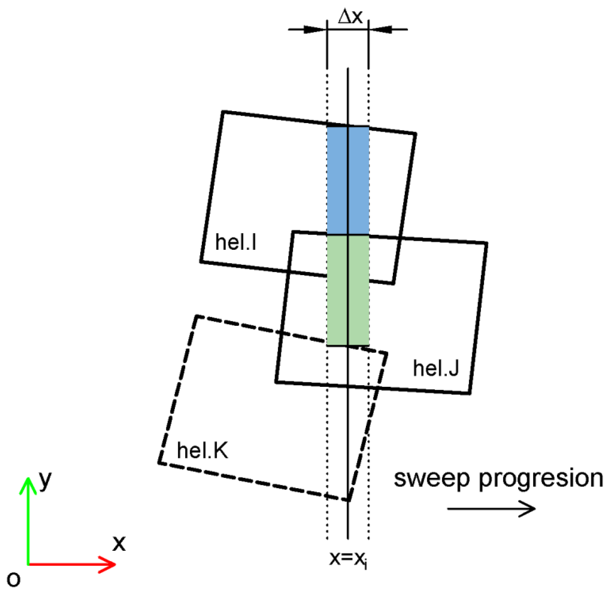
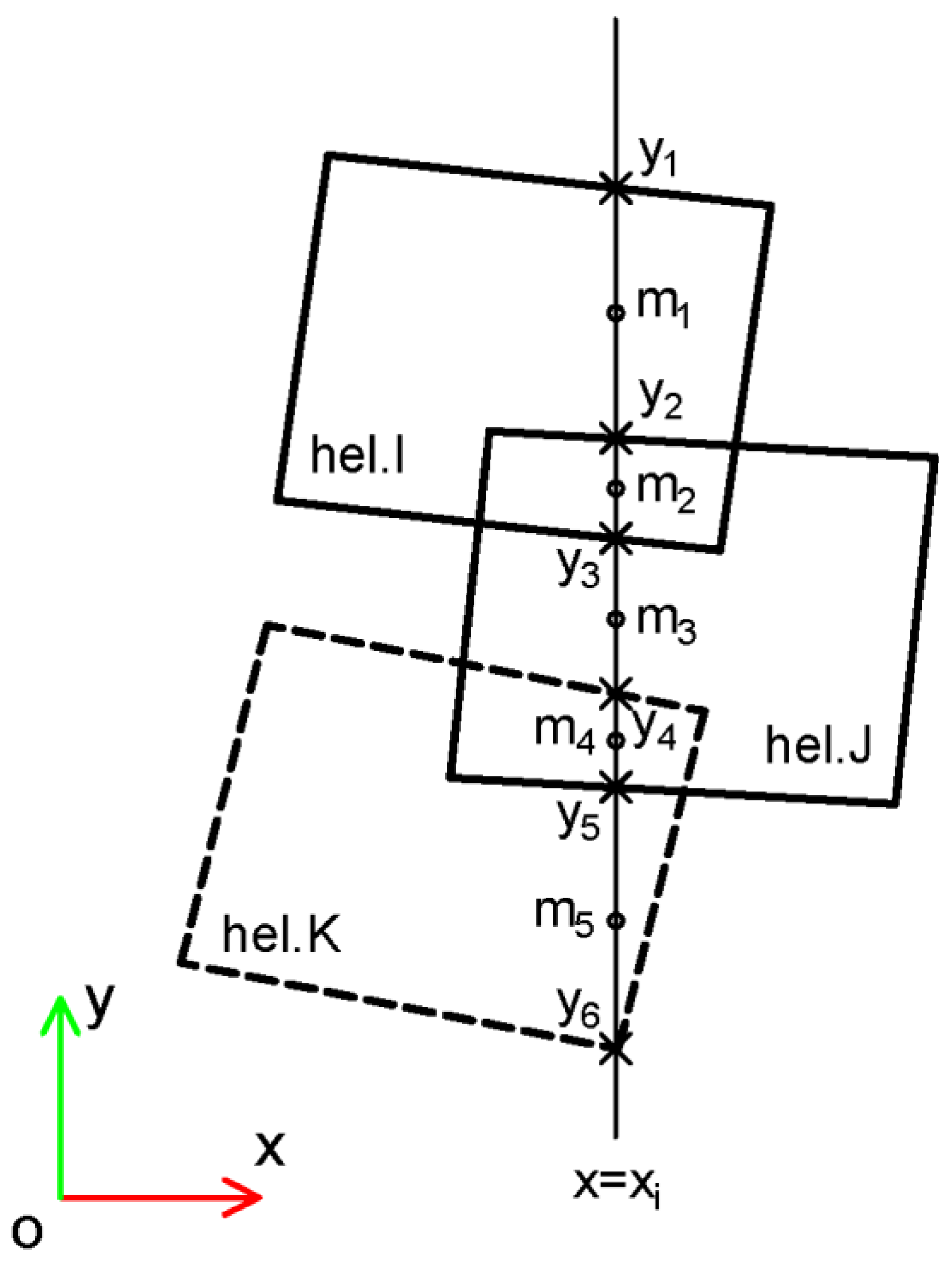
2.2.2. Numerical Integration by Vertical Stripes (GM2)

The GM2 method can be considered a particular case of the GM1 method when n → ∞.
The procedure for obtaining the shading and blocking efficiency can be summarized as follows:
  • m points xi are considered with uniform separation Δx along the x-axis.
  • An iterative process is started that goes through the m values of xi.
2.1. The heliostats cut by the line x = xi are selected. In general, s and b heliostats projected by shading and blocking, respectively (Figure 7). The coordinates yu and yl of the upper and lower cutting points, respectively, of each of the selected heliostats are obtained when cut by the line x = xi.
2.2. The (s + b) values obtained in step (2.1) are ordered from highest to lowest, obtaining (s + b) − 1 portions on the line x = xi. Additionally, the column matrices M and L are obtained, which contain the y-coordinate of the midpoints and the lengths, respectively, of the aforementioned portions. Finally, by using expression (13) the logical matrix A, of (s + b) − 1 rows and (s + b) columns, which expresses the membership of the midpoints of each portion to each heliostat, is obtained.
A = y l t < M     M < y u t
2.3. Analogous to the GM1 method.
2.4. Analogous to the GM1 method.
2.5. The useful and total reflecting area, in the abscissa x = xi, of an arbitrary heliostat that occupies column r can be calculated, respectively, through the relationships (14) and (15):
( s u ) x = x i = x · B , C r L
s x = x i = x · A , C r L
This processes all the selected heliostats simultaneously.
3.
Once the m values of xi have been processed, the shading and blocking efficiency of the solar field can be determined through the relationships (7) and (8).

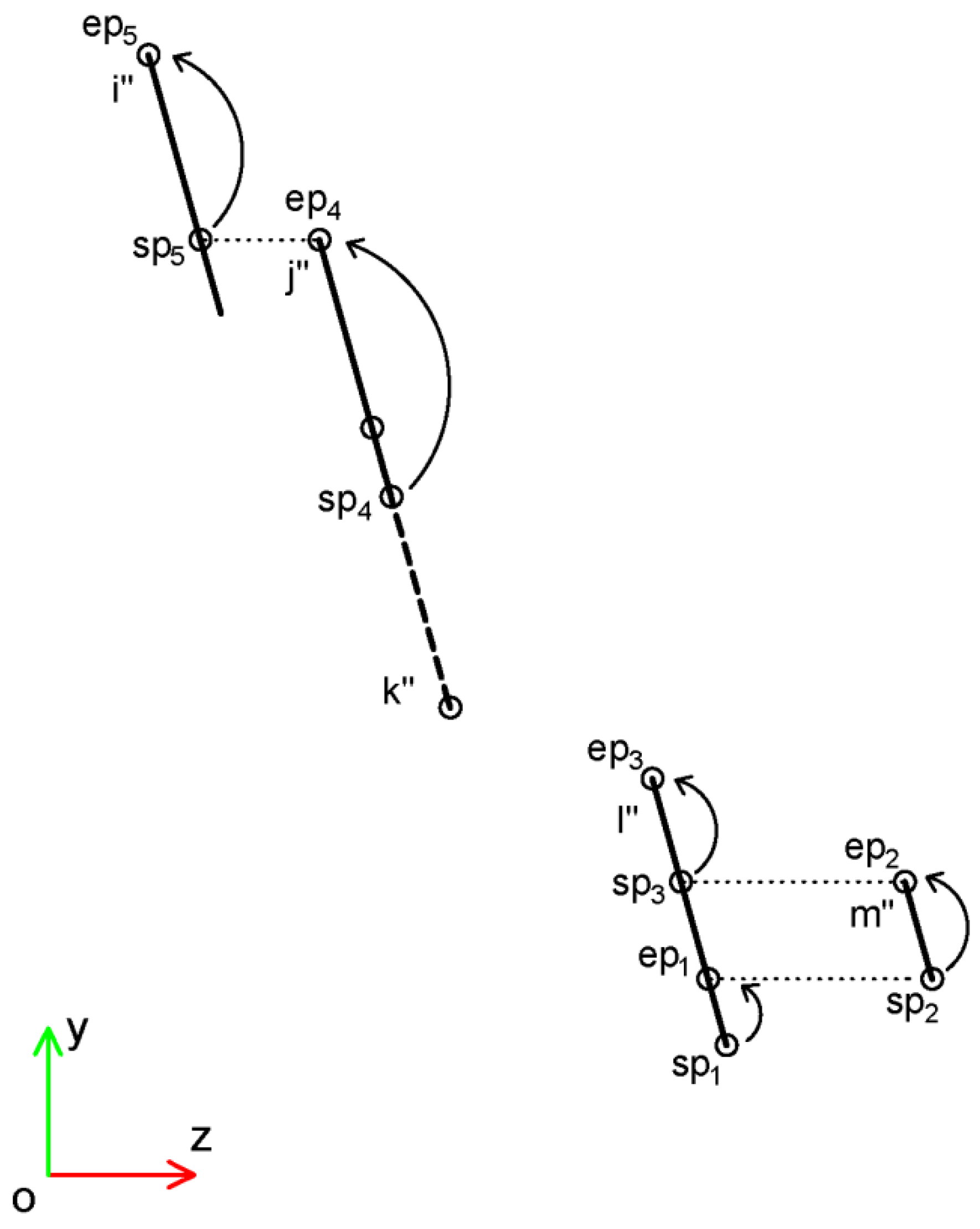
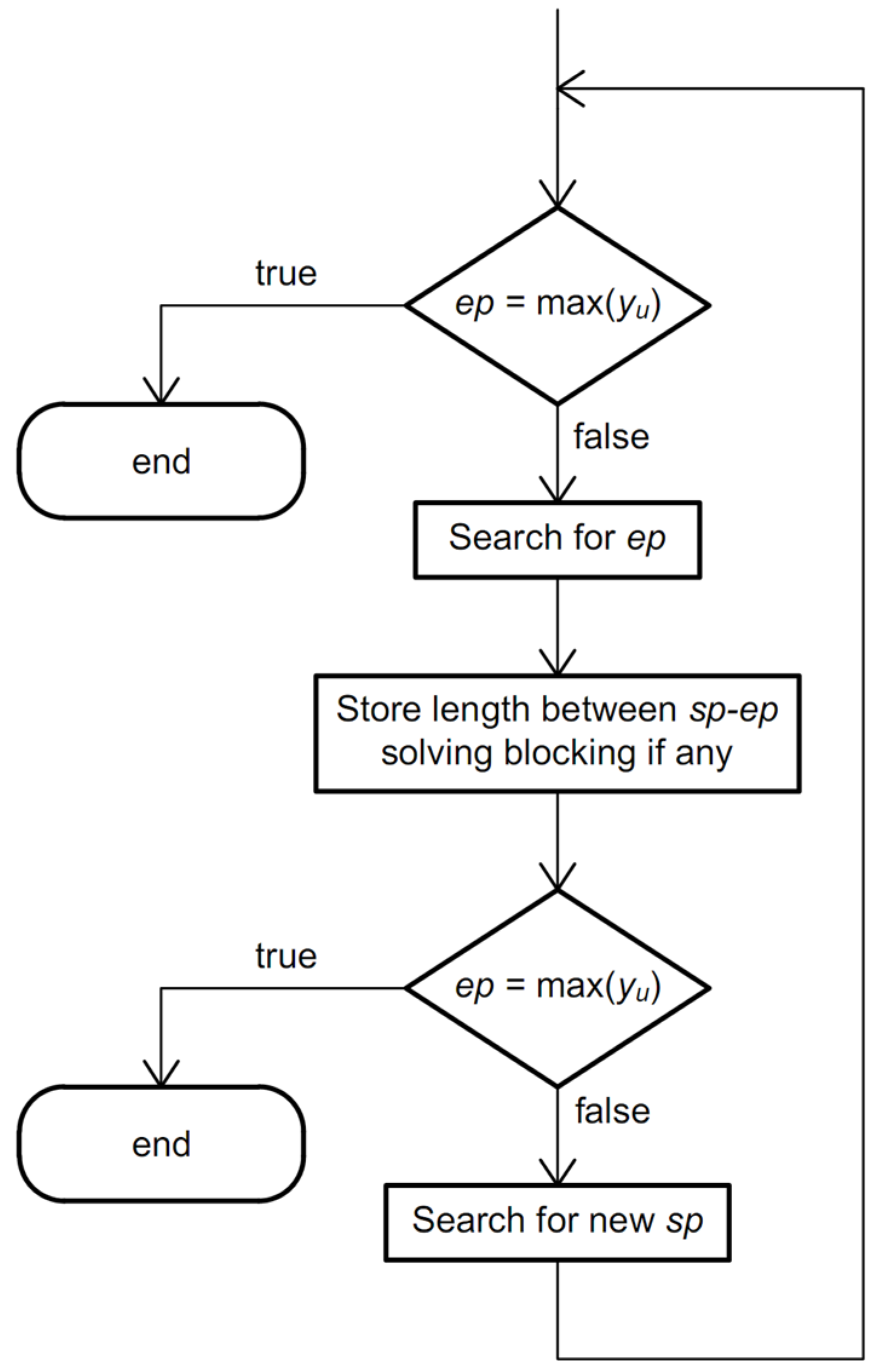
2.2.3. Starting Point (GM3)

Let i”, j”, k”, l”, and m” be the graphical representation on the oyz plane of the segments originated by sectioning five arbitrary heliostats by means of the plane parallel to the oxz containing the line x = xi (Figure 8).
The procedure for obtaining the shading and blocking efficiency can be summarized as follows:
  • Analogous to GM2.
  • An iterative process is started that goes through the m values of xi.
2.1. Analogous to GM2.
2.2. Locate the first starting point sp1.
2.3. The following nested iterative process is performed (Figure 9):

Considerations about the Algorithm

Termination condition: The termination condition is true when ep = max(yu).
Regarding the starting point, sp: sp1 = min(yl). For the second and following:
If ep = yu then there are two cases:
  • If there is a higher segment (with a higher z-coordinate) than the current segment and yl ≤ ep ≤ yu, where yl and yu correspond to the aforementioned highest segment, then sp = ep (e.g., sp3 or sp5).
  • Otherwise, sp = min(yl) (e.g., sp4).
Otherwise: sp = min(yl) of the higher segments than the current segment (e.g., sp2).
Regarding the end point, ep:
  • ep = min(yl) of the higher segments than the current segment, as long as ylmin(yl)yu, where yl and yu correspond to the current segment (e.g., ep1).
  • Otherwise, ep = yu of the current segment (e.g., ep2, ep3, ep4 and ep5).
Regarding blocking:
If there are candidates for blocking associated with the current segment, a logical matrix is obtained by applying steps (2.2) and (2.4) in the GM2 method, with s = 1 (involving the unshaded fragment between sp and ep of the current segment) and all blocking candidates related to it. Finally, an expression analogous to (5) is applied to determine the useful reflecting area. Where there are no blocking candidates, the useful reflecting area can be calculated by the product Δ(yepysp).
Once the m values of xi have been processed, the shading and blocking efficiency of the solar field can be determined through the relationships (7) and (8).

3. Results

The models selected for comparison purposes have certain specific characteristics that help to foreground the main advances of these new models.
M3 (homology) was the fastest and most accurate of the five methods proposed and analyzed in [35]. It is a ray-tracing method characterized by solving the most computationally expensive processes—line-plane intersection and point-in-polygon check—through the application of homographic transformations. M4 [35] (Boolean operations between flat regions) is included as an example of a methodology characterized by offering accurate and precise results regardless of the resolution used.
An additional method, M0, based on MCRT [35], was also chosen as a reference due to its great accuracy at high resolutions. The main characteristics of this method are indicated below:
  • It uses MCRT methodology.
  • It considers the surface of the heliostat as a rectangular shape and a quadric elliptic curvature without gaps (a sphere or a paraboloid) with canting on-axis.
  • The incident rays are generated randomly following a particular sunshape model.
  • The points of application of the incident rays are generated randomly with a uniform distribution on the surface of the heliostat.
  • It considers the optical errors (macroscopic and microscopic) associated with the reflective surface of the heliostat as applied in a non-deterministic way, using Gaussian distributions in both cases.
  • The reflectivity of the heliostat, as well as the losses due to atmospheric attenuation, are applied in a non-deterministic way.
All the methods under analysis, except for M0, use the same candidate selection or filtering algorithm developed in [40], with the filtering level F1 + F2 in both shading and blocking. It should be noted that the aforementioned candidate selection methodology does not limit their number and that all the candidates, after the application of the two filters, produce real shading and blocking. In the case of M0, the candidate selection methodology described in [35] is used, which allows for the expansion of the candidate analysis spectrum by applying a homothetic factor greater than one. (For the purposes of this comparison, the method used to obtain the reference case (M0) uses a Gaussian sunshape model, with σ = 2.325 mrad, with the result that the incident and reflected rays have greater deviations than in the other cases.). The computation times presented below include the execution time of the candidate filtering.
Furthermore, data from the case study have been selected to have large shading and blocking (low solar altitude, relatively low target height, and compact layout). In this respect, it was verified that, after the application of the F1 + F2 selection filters, the number of candidates for shading and blocking was 19,908 and 4,637, respectively, and the computation time required for the F1 + F2 filtering was 0.231 s. The main characteristics of the test field used in this comparison are indicated in Table 2.
With the exception of M4, the results of all the methods depend on the resolution set. For this reason, the results will be analyzed using the following eight resolution levels: Nc = 5 × 5, 10 × 10, 20 × 20, 40 × 40, 80 × 80, 160 × 160, 320 × 320, and 640 × 640. The RMSE (Root Mean Square Error) is used to determine the deviations between the method under analysis and the reference case:
R M S E = i = 1 i = N η i η R i 2 N    
where ηi and ηRi are the shading and blocking efficiency, expressed as a percentage ratio, of the ith heliostat calculated by the method under study and the reference case, respectively, and N is the number of heliostats in the field.
Table 3 shows the main data used to obtain the reference case.
Figure 10 shows the RMSE values as a function of the number of calculation points Nc or number of traced rays.
The deviation for M4 is constant (0.174%) and independent of the resolution used, while the deviations for the others are reduced as the resolution increases. For M0, the reduction in error is progressive as the resolution increases. It can be observed that the error is reduced by half when the number of traced rays is quadrupled. It is the most accurate method at high resolutions, but also one of the least accurate at low and medium resolutions. On the other hand, methods GM1, GM2, GM3, and M3 tend towards the results of M4 as the resolution is increased because they all share the same initial hypotheses. How they approach the asymptote defined by M4 is different, however. In the case of M3, the approach is made following a practically straight line with a negative, constant slope. Like M0, errors are reduced by approximately half when the resolution is quadrupled, until approximately Nc = 80 × 80. Then, a transition zone appears until the asymptote is reached at around Nc = 320 × 320. In the case of GM1, the number of errors is greater than those of M0 and M3 at low resolutions, but the number of errors reduces faster with the increase in resolution. Like M3, the asymptote is reached at around Nc = 320 × 320.
The global methods GM2 and GM3 present coincident graphs, since the shading and blocking efficiency of each of the heliostats in the field is identical in both methods. At low resolutions, the deviation follows a curve whose slope is decreasing, reaching the asymptote around Nc = 80 × 80. Both methods have lower deviations than GM1, M0, and M3. The least accurate method at low resolutions is GM1 due to the poor accuracy of the method at the edges of the heliostats caused by the excessive size of the grid. Figure 11 shows the not-shaded (blue) and blocked (cyan) surface of heliostat 22 in the sample field, obtained using GM1, with the grid lines of the adjacent heliostats disabled to improve the clarity of the figure. It can be seen that the grid adjustment at the edges of the heliostats improves as the resolution is increased.
Figure 12 shows the computation times as a function of the number of calculation points Nc or the number of traced rays.
All simulations were executed on the same computer, with an Intel i7-5820 K 3.3 GHz hexa-core processor and 32 GB RAM. In every case, parallel processing was disabled.
The M4 computation time is independent of the required resolution (9.87 s). The computation times for the other methods increase with resolution. While in the cases of GM2 and GM3 the association with the resolution is linear, this is not the case with GM1, M0, and M3. GM2 is between 1.5 and 2.1 times faster than GM3 at an equal resolution. This is because, as described in Section 2.2.3, the GM3 algorithm consists of a nested while loop within a for-type loop, which is less efficient than the algorithm used by GM2, which is free of the nested loop.
The fastest method for low resolutions to resolutions of approximately Nc = 50 × 50 is GM1, closely followed by GM2 with a very similar performance. From Nc = 50 × 50 to Nc = 140 × 140, the fastest methods are GM2 and M3, with practically identical performances. Finally, above the resolution Nc = 260 × 260 the fastest method is M4.
The information in Figure 10 and Figure 12 needs to be more comprehensive to determine the choice of the most appropriate methodology in applications focused on heliostat field design and optimization, as this must combine low computation times and deviations. For this reason, Figure 13 plots the RMSE values as a function of the computation time for each method. In the cases of GM2 and GM3, three new simulations were added, corresponding to Nc = 2 × 2, 3 × 3, and 4 × 4, to complete the upper left part of the chart. Three different regions can be distinguished:
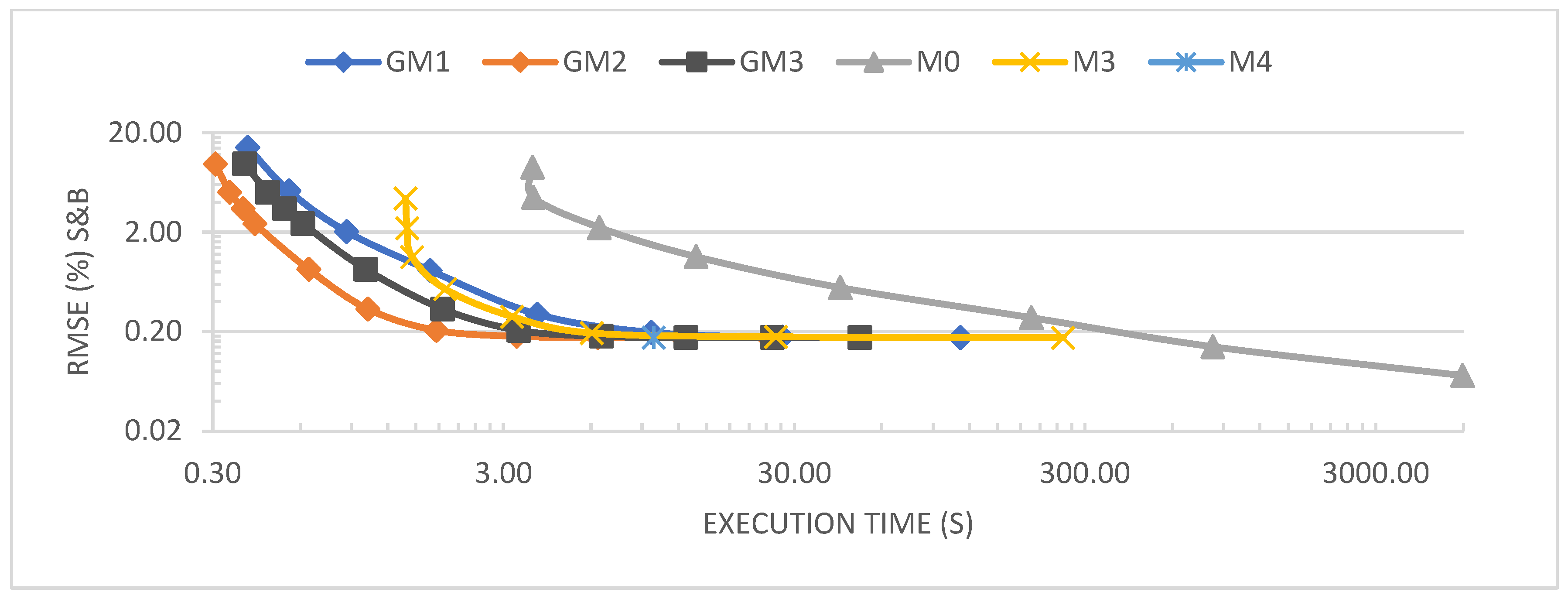
  • Above the ordinate corresponding to RMSE = 0.18%, the most appropriate method is GM2 followed by GM3. In this range, GM2 is between 1.62 and 8.19 times faster than GM1, between 1.46 and 1.96 times faster than GM3, between 3.83 and 7.80 times faster than M3, and between 10.6 and 194 times faster than M0.
  • In the range of RMSE values between 0.174 and 0.18%, the fastest method is M4 followed by GM2.
  • Finally, in the lower zone, if deviations below 0.174% are desired, the only valid method is M0, although at the cost of very high computation times.
Table 4 shows the shading and blocking efficiency of the solar field evaluated at three of the resolutions analyzed (Nc = 5 × 5, 10 × 10, and 640 × 640). The results corresponding to the reference case obtained with M0 are indicated by the mean and standard deviation of a total of ten executions with the same initial data, as this method consists of several non-deterministic sub-processes.
A notable result is that the efficiency value obtained by GM2 − GM3 at the lowest resolution analyzed coincides in its first four significant digits with the results obtained by M4 which, as noted above, establishes the limit case. It can thus be affirmed that the GM2 and GM3 methods are very accurate even at low resolutions.
Table 4 also shows that all the results obtained at Nc = 640 × 640 (the highest resolution used in the test) are lower than those obtained by the reference case. This discrepancy is due to the initial hypotheses used. It has been proven, by making adaptations to the M0 algorithm, that the only initial hypothesis affecting the deviation is hypothesis (i) the surface of the heliostats is a flat rectangular sheet. Conversely, it has been proven that hypotheses (ii) the sunshape model is a point source Sun and (v) all the rays reflected by a heliostat converge precisely at the center of the target, individually, do not have an impact on the deviation observed. (The M0-MCRT code configured with hypothesis (ii) is obtained: η   ¯ = 0.407949 and σ = 2.51 × 10⁻⁶; while with hypothesis (v) it is obtained: η   ¯ = 0.407953 and σ = 2.07 × 10⁻⁶).
Finally, regarding the candidate selection or filtering algorithm, the following considerations should be made:
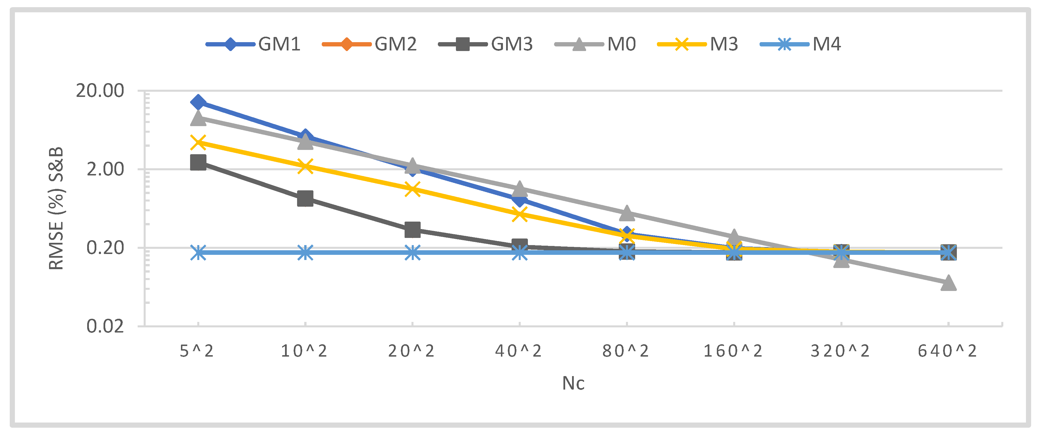
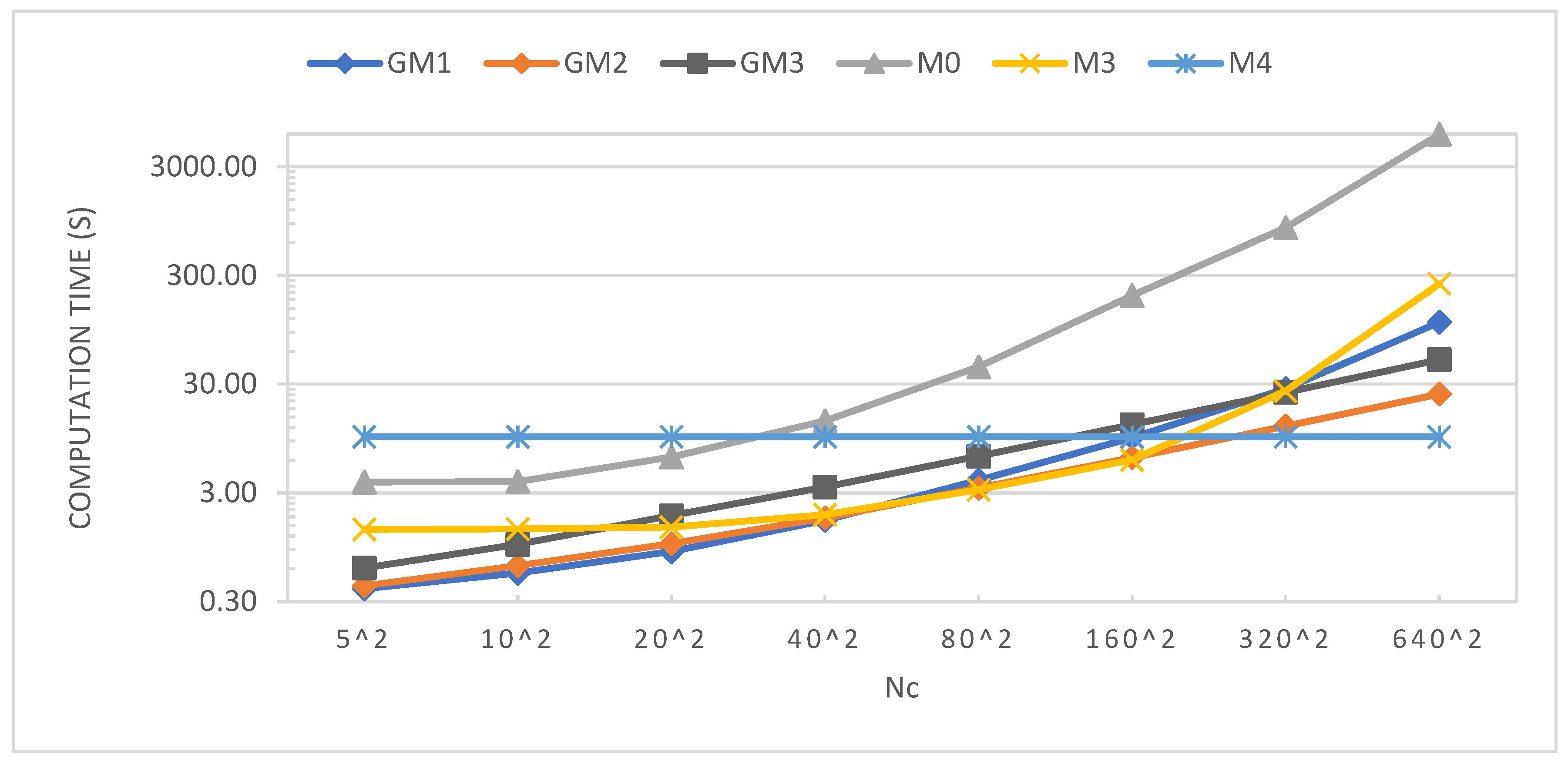
  • With the level of filtering used (F1 + F2 filters for both shading and blocking), the numbers of candidates for shading and blocking were 19,908 and 4,637, respectively. At the lowest resolution analyzed (Nc = 5 × 5), the computation times for GM2, M3, and M4 were 0.42, 1.38, and 9.38 s, respectively.
  • If a less demanding filtering level is applied (F1 filter for both shading and blocking), the computation times for GM2, M3, and M4 would become 0.39, 1.78, and 10.83 s, respectively. This results in a reduction in the computation time of the global method of 7.1%, but a corresponding increase in the computation times of M3 and M4 of 29.0% and 15.5%, respectively, due to the increase in the number of candidates to be processed. Specifically, the number of candidates for shading and blocking in this case are 26,512 and 6,681, respectively.

4. Discussion and Conclusions

In this paper, three global methods for the determination of the shading and blocking efficiency in CRSs are presented: discretization in elementary rectangles, numerical integration by vertical stripes, and starting point. These methods determine the useful and total reflecting areas, have low computation times and minimum errors, and are designed to be implemented in codes focused on heliostat field design and optimization. The methods were compared with two outstanding “individual” methods (homology and Boolean operations) using, as a reference case, the results obtained by a sixth method based on the MCRT technique at a high resolution. The numerical integration by vertical stripes method showed the lowest error values and highest computation speed, being, at the same error level, between 1.62 and 8.19 times faster than the discretization in elementary rectangles method, between 1.46 and 1.96 times faster than the starting point method, between 3.83 and 7.80 times faster than the homology method, and between 10.6 and 194 times faster than the method based on the MCRT technique. As the resolution increased, the results of the proposed methods converged with those obtained by Boolean operations, while they all showed an offset in comparison with the reference case, due mainly to the assumption of a flat rectangular sheet for the surface of the heliostats.

Author Contributions

Methodology, G.O.; Software, G.O.; Formal analysis, G.O.; Writing—original draft, G.O.; Writing—review & editing, R.B. and A.R.; Supervision, A.R.; Project administration, A.R.; Funding acquisition, A.R. All authors have read and agreed to the published version of the manuscript.

Funding

The authors acknowledge the financial support of the Spanish Ministry of Science and Innovation to the PID2019-110283RB-C31 project.

Data Availability Statement

Data are contained within the article.

Conflicts of Interest

The authors declare no conflict of interest.

References

  1. Garcia, P.; Ferriere, A.; Bezian, J.-J. Codes for solar flux calculation dedicated to central receiver system applications: A comparative review. Sol. Energy 2008, 82, 189–197. [Google Scholar] [CrossRef]
  2. Cruz, N.C.; Redondo, J.L.; Berenguel, M.; Álvarez, J.D.; Ortigosa, P.M. Review of software for optical analyzing and optimizing heliostat fields. Renew. Sustain. Energy Rev. 2017, 72, 1001–1018. [Google Scholar] [CrossRef]
  3. Blanco, M.J.; Amieva, J.M.; Mancilla, A. The TONATIUH software development project: An open source approach to the simulation of solar concentrating systems. In Proceedings of the 2005 ASME International Mechanical Engineering Congress and Exposition, Orlando, FL, USA, 5–11 November 2005. [Google Scholar]
  4. Wendelin, T. SolTRACE: A New Optical Modeling Tool for Concentrating Solar Optics. In Proceedings of the National Renewable Energy Laboratory (NREL), International Solar Energy Conference, Kohala Coast, HI, USA, 15–18 March 2003. [Google Scholar]
  5. Leary, P.L.; Hankins, J.D. Users Guide for MIRVAL: A Computer Code for Comparing Designs of Heliostat-Receiver Optics for Central Receiver Solar Power Plants; Sandia Report SAND-77-8280; Sandia National Lab.: Livermore, CA, USA, 1979. [Google Scholar]
  6. Belhomme, B.; Pitz-Paal, R.; Schwarzbözl, P.; Ulmer, S. A New Fast Ray Tracing Tool for High-Precision Simulation of Heliostat Fields. J. Sol. Energy Eng. 2009, 131, 031002. [Google Scholar] [CrossRef]
  7. Duan, X.; He, C.; Lin, X.; Zhao, Y.; Feng, J. Quasi-Monte Carlo ray tracing algorithm for radiative flux distribution simulation. Sol. Energy 2020, 211, 167–182. [Google Scholar] [CrossRef]
  8. Gebreiter, D.; Weinrebe, G.; Wöhrbach, M.; Arbes, F.; Gross, F.; Landman, W. sbpRAY—A fast and versatile tool for the simulation of large scale CSP plants. AIP Conf. Proc. 2019, 2126, 170004. [Google Scholar]
  9. Lipps, F.W.; Vant-Hull, L. Shading and Blocking Geometry for a Solar Tower Concentration with Rectangular Mirrors; ASME Paper 74-WA/sol-11; American Society of Mechanical Engineers, Winter Annual Meeting: New York, NY, USA, 1974. [Google Scholar]
  10. Lipps, F.W. The shading and blocking processor and the receiver model. In ERDA Workshop on Methods for Optical Analysis of Central Receiver Systems; University of Houston: Houston, TX, USA, 1977. [Google Scholar]
  11. Lipps, F.W. Computer Simulation of Shading and Blocking: Discussion of Accuracy and Recommendations NREL/TP-253-4281; National Renewable Energy Laboratory: Golden, CO, USA, 1992. [Google Scholar]
  12. Lipps, F.; Vant-Hull, L. A cellwise method for the optimization of large central receiver systems. Sol. Energy 1978, 20, 505–516. [Google Scholar] [CrossRef]
  13. Lipps, F.W.; Vant-Hull, L. A Programmer’s Manual for the University of Houston Computer Code RCELL: Cellwise Optimization for the Solar Central Receiver Project; Tech. Rep., SAND 0763-1; University of Houston: Houston, TX, USA, 1980. [Google Scholar]
  14. McFee, R.H. Computer Program CONCEN for Calculation of Irradiation of Solar Power Central Receiver. In ERDA Workshop on Methods for Optical Analysis of Central Receiver Systems; University of Houston: Houston, TX, USA, 1977. [Google Scholar]
  15. Kistler, B.L. A User’s Manual for DELSOL3: A Computer Code for Calculating the Optical Performance and Optimal System Design for Solar Thermal Central Receiver Plants; Sandia National Labs Report SAND86-8018; Sandia National Lab.: Livermore, CA, USA, 1986. [Google Scholar]
  16. Wagner, M.J.; Wendelin, T. SolarPILOT: A power tower solar field layout and characterization tool. Sol. Energy 2018, 171, 185–196. [Google Scholar] [CrossRef]
  17. Wei, X.; Lu, Z.; Lin, Z.; Zhang, H.; Ni, Z. Optimization procedure for design of heliostat field layout of a 1MWe solar tower thermal power plant. In Solid State Lighting and Solar Energy Technologies; SPIE—The International Society for Optical Engineering: Bellingham, WA, USA, 2008; Volume 6841. [Google Scholar]
  18. Yu, Q.; Wang, Z.; Xu, E.; Zhang, H.; Lu, Z.; Wei, X. Modeling and simulation of 1MWe solar tower plant’s solar flux distribution on the central cavity receiver. Simul. Model. Pract. Theory 2012, 29, 123–136. [Google Scholar] [CrossRef]
  19. Noone, C.J.; Torrilhon, M.; Mitsos, A. Heliostat field optimization: A new computationally efficient model and biomimetic layout. Sol. Energy 2012, 86, 792–803. [Google Scholar] [CrossRef]
  20. Cruz, N.C.; Redondo, J.L.; Berenguel, M.; Álvarez, J.D.; Becerra-Teron, A.; Ortigosa, P.M. High performance computing for the heliostat field layout evaluation. J. Supercomput. 2016, 73, 259–276. [Google Scholar] [CrossRef]
  21. Sassi, G. Some notes on shadow and blockage effects. Sol. Energy 1983, 31, 331–333. [Google Scholar] [CrossRef]
  22. Collado, F.J.; Guallar, J. Campo: Generation of regular heliostat fields. Renew. Energy 2012, 46, 49–59. [Google Scholar] [CrossRef]
  23. Collado, F.J.; Guallar, J. A review of optimized design layouts for solar power tower plants with campo code. Renew. Sustain. Energy Rev. 2013, 20, 142–154. [Google Scholar] [CrossRef]
  24. Besarati, S.M.; Goswami, D.Y. A computationally efficient method for the design of the heliostat field for solar power tower plant. Renew. Energy 2014, 69, 226–232. [Google Scholar] [CrossRef]
  25. Wang, J.; Duan, L.; Yang, Y. An improvement crossover operation method in genetic algorithm and spatial optimization of heliostat field. Energy 2018, 155, 15–28. [Google Scholar] [CrossRef]
  26. Wang, J.; Duan, L.; Yang, Y.; Yang, L. Rapid design of a heliostat field by analytic geometry methods and evaluation of maximum optical efficiency map. Sol. Energy 2019, 180, 456–467. [Google Scholar] [CrossRef]
  27. Rizvi, A.A.; Yang, D. A detailed account of calculation of shading and blocking factor of a heliostat field. Renew. Energy 2021, 181, 292–303. [Google Scholar] [CrossRef]
  28. Huang, W.; Li, L.; Li, Y.; Han, Z. Development and evaluation of several models for precise and fast calculations of shading and blocking in heliostats field. Sol. Energy 2013, 95, 255–264. [Google Scholar] [CrossRef]
  29. Ortega, G.; Rovira, A. A fast and accurate methodology for the calculation of the shading and blocking efficiency in central receiver systems. Renew. Energy 2020, 154, 58–70. [Google Scholar] [CrossRef]
  30. Arrif, T.; Sánchez-González, A.; Bezza, B.; Belaid, A. Shadowing and Blocking Factors in Heliostats: Comparison between Parallel and Oblique Projections. AIP Conf. Proc. 2022, 2445, 120004. [Google Scholar] [CrossRef]
  31. Raj, M.; Bhattacharya, J. An accurate and cheaper method of estimating shading and blocking losses in a heliostat field through efficient filtering, removal of double counting and parallel plane assumption. Sol. Energy 2022, 243, 469–482. [Google Scholar] [CrossRef]
  32. Belaid, A.; Filali, A.; Hassani, S.; Arrif, T.; Guermoui, M.; Gama, A.; Bouakba, M. Heliostat field optimization and comparisons between biomimetic spiral and radial-staggered layouts for different heliostat shapes. Sol. Energy 2022, 238, 162–177. [Google Scholar] [CrossRef]
  33. Zhang, M.; Yang, L.; Xu, C.; Du, X. An efficient code to optimize the heliostat field and comparisons between the biomimetic spiral and staggered layout. Renew. Energy 2015, 87, 720–730. [Google Scholar] [CrossRef]
  34. Biggs, F.; Vittitoe, C.N. The Helios Model for the Optical Behaviour of Reflecting Solar Concentrators; SAND76-0347; Sandia National Lab.: Albuquerque, NM, USA, 1979. [Google Scholar]
  35. Ortega, G.; Rovira, A. Proposal and analysis of different methodologies for the shading and blocking efficiency in central receivers systems. Sol. Energy 2017, 144, 475–488. [Google Scholar] [CrossRef]
  36. Ramos, A.; Ramos, F. Heliostat blocking and shadowing efficiency in the video-game era. arXiv 2014, arXiv:1402.1690. [Google Scholar]
  37. Kim, S.; Lee, I.; Lee, B.J. Development of performance analysis model for central receiver system and its application to pattern-free heliostat layout optimization. Sol. Energy 2017, 153, 499–507. [Google Scholar] [CrossRef]
  38. Manson, D.S. Determination of areas and volumes of intersection of zones in old and new grids. In Appendix B in the TOOREZ Lagrangian Rezoning Code, SLA-73-1057; Thorne, B.J., Holdridge, B.B., Eds.; Sandia Laboratories: Albuquerque, NM, USA, 1974. [Google Scholar]
  39. Yao, Y.; Hu, Y.; Gao, S. Heliostat field layout methodology in central receiver systems based on efficiency-related distribution. Sol. Energy 2015, 117, 114–124. [Google Scholar] [CrossRef]
  40. Ortega, G.; Rovira, A. A new method for the selection of candidates for shading and blocking in central receiver systems. Renew. Energy 2020, 152, 961–973. [Google Scholar] [CrossRef]
Figure 1. Illustration of the orthogonal cylindrical projection of the vertices of heliostat A on the oxy plane according to So.
Energies 17 01282 g001
Figure 2. Illustration of the central projection of the vertices of heliostat B onto the plane defined by heliostat A.
Energies 17 01282 g002
Figure 3. Result of the projection process on an example field with a radial stagger arrangement of 48 heliostats at the autumn equinox at 8:00 a.m.
Energies 17 01282 g003
Figure 4. Scheme of the global methods for calculating the shading and blocking efficiency. The blue and green rectangles represent the useful reflecting areas of heliostats I and J, respectively, for the abscissa x = xi.
Energies 17 01282 g004
Figure 5. Scheme of the method based on discretization in elementary rectangles (GM1).
Energies 17 01282 g005
Figure 6. The result obtained by the discretization in elementary rectangles method (GM1), with Nc = 5 × 5, for the example heliostat field at the autumn equinox at 6:30 a.m.
Energies 17 01282 g006
Figure 7. Scheme of the method based on numerical integration by vertical stripes (GM2).
Energies 17 01282 g007
Figure 8. Scheme of the method based on the starting point (GM3).
Energies 17 01282 g008
Figure 9. Flowchart of the nested iterative process (GM3).
Energies 17 01282 g009
Figure 10. The RMSEs associated with the shading and blocking efficiency of each of the techniques based on Nc. The vertical axis is in a logarithmic scale.
Energies 17 01282 g010
Figure 11. The GM1 results for heliostat 22 in the example heliostat field. Autumn equinox at 6:30 a.m. Left Nc = 5 × 5; right Nc = 20 × 20.
Energies 17 01282 g011
Figure 12. The execution time in seconds of each of the techniques based on Nc. The vertical axis is in a logarithmic scale.
Energies 17 01282 g012
Figure 13. RMSE vs. execution time. Both axes in logarithmic scale.
Energies 17 01282 g013
Table 1. Initial hypotheses on which the methods based on projection are frequently based.
(i) The surface of the heliostat is a flat rectangular sheet.
(ii) The sunshape model considered is a point source sun.
(iii) Optical errors are null.
(iv) The neighboring heliostats are parallel to the one under consideration.
(v) All the rays reflected by a heliostat are directed exactly to the center of the target.
Table 2. Test field data.
Day number and solar hour263.5 (autumn equinox) at 6:30 a.m.
Latitude37°18′51″
Cylindrical tower (diameter × height)12 m × 142 m
Receiver Regular prism; 12 sides inscribed in a circle of 10 m diameter and 16 m height
Heliostats (width × height)12.0 m × 10.0 m
Heliostat center height6.0 m
Heliostat surface Spherical for method M0 and flat for the rest
CantingOn-axis for method M0
Target height150.0 m
Heliostat layoutSurrounding field constant angle alternating polar arrangement of 4,238 heliostats (50 rows)
Table 3. Data for the reference case.
Method M0—MRCT
Sunshape modelGaussian with σ = 2.325 mrad
Slope error0 mrad
Specularity error0 mrad
Number of rays5 × 106 rays per heliostat
Heliostat surfaceSpherical
CantingOn-axis
Table 4. The shading and blocking efficiency of the solar field for each method.
Nc = 5 × 5Nc = 10 × 10Nc = 640 × 640
GM10.3968070.4079380.407503
GM2 − GM30.4074900.4074860.407505
M30.4132420.4094670.407511
M4 0.4075050.4075050.407505
REF − M0 η ¯ = 0.407953, σ = 2.45 × 10⁻⁶ (Nr = 5 × 10⁶ rays)
Disclaimer/Publisher’s Note: The statements, opinions and data contained in all publications are solely those of the individual author(s) and contributor(s) and not of MDPI and/or the editor(s). MDPI and/or the editor(s) disclaim responsibility for any injury to people or property resulting from any ideas, methods, instructions or products referred to in the content.

