A Novel Method for Removal of Dual Decaying DC Offsets to Enhance Discrete Fourier Transform-Based Phasor Estimation

Abstract

This paper presents a novel method for the removal of dual decaying DC offsets (DDCOs) to enhance discrete Fourier transform-based phasor estimation. The method proposed in this paper uses the sum of even samples and the sum of odd samples from the input signal to remove the AC components, thereby precisely estimating the primary and secondary DDCOs. The fluctuations induced by DCCOs present in the output of traditional DFT methods are eliminated by using the estimated DCCOs. The performance of the method was evaluated in terms of both mathematical-generated signals and fault current signals from a 154 kV Korean overhead transmission system. PSCAD/EMTDC was used to generate fault current signals at various fault distances and angles. The results show that the proposed method can estimate the phasor of the fundamental frequency component accurately regardless of the primary and secondary DCCOs. The paper concludes by describing the hardware implementation in a prototype unit that considers the real-world requirements of power system protection.

1. Introduction

Accurate and fast phasor estimation is essential for efforts to protect power systems. The discrete Fourier transform (DFT) is well known to effectively estimate phasors. However, the fault current signal is contaminated by decaying DC offsets (DDCOs), thereby compromising the accuracy and convergence speed of the DFT [1,2]. Various methods have been used to remove DDCOs from fault current signals [3]. Assuming that DDCO exhibited a specific time constant, DDCO was completely removed by a Kalman filter in [4,5] and a digital mimic filter in [6]. However, the time constants of the filters must lie within certain ranges. If the assumed time constant is not the actual constant, the estimates are erroneous.

Least error squares (LES) methods have been used to suppress DDCO over certain ranges of time constants [7,8,9,10,11,12,13,14,15]. The authors in [7] used the first three terms of the Taylor series expansion to linearize DDCO, followed by the application of a simple LES curve-fitting technique to estimate the magnitude of both DDCO and each harmonic contained in the signal (only the fundamental and third harmonic were considered because this method utilized a low-pass filter to eliminate higher-order harmonics). In [4], Kalman filters were used to remove DDCOs, with two-state and three-state Kalman filters used to estimate the voltage phasor and current phasor, respectively. In [8,9], the recursive LES, which is an improved method over the non-recursive LES in [7], was used to estimate the Fourier coefficients of the input waveform. These methods require fewer computations compared to the method proposed in [7]. The methods in [10,11] calculate the coefficients of a digital filter using the weighted error squares and the forgetting factor. The forgetting factor determines the window size; the smaller the forgetting factor, the smaller the window size. In [12], DDCO is identified by applying the LES-based method to the Prony analysis expression. A non-linear LS method was employed with RMS–wavelet in [13] to estimate DDCO. The LES-based approach was applied after computing the RMS–wavelet, and the simulation was completed using an iterative algorithm. In [14], the LES-based method was applied to estimate the phasor of the current signal, considering the response of the current transformer. Although these methods do not require knowledge of the time constant, the efficacy of such methods diminished as Taylor series expansion was used for linearization.

A deep neural network (DNN) was used to manage the problems that arise when filters do not adequately manage different time constants, noise, and harmonics during DDCO removal [15,16,17]. The method in [15] uses the multilayer perceptron architecture to predict both current and voltage signals. Subsequently, it computes the complex apparent impedance through an ongoing online training process. In [16], mathematically generated fault current signals under various conditions were generated for training the DNN model. Consequently, the model can be used to remove DDCO from the fault current signal; thus, such DNNs are often effective. The method of [17] also used a DNN to remove DDCO from the fault current waveform, but fewer samples were required (less than one cycle). However, practicality is a concern; the deep layers of DNNs impose high computational burdens. Because the networks are trained offline, certain errors might arise in various environments, such as changes in the voltage level. DNNs would be more effective if it were possible to train them online; this would allow rapid adaptation to a new environment.

Many efforts have been made to eliminate DDCO using the modified discrete Fourier transform (MDFT). The MDFT, as described in [2], uses three successive DFT outputs to estimate DDCO. This approach solves the problem imposed by unknown time constants. However, the convergence time is less responsive; N + 2 samples are required. The same authors proposed a modified half-cycle DFT (MHCDFT) that requires only N/2 + 2 samples. Such algorithms are not sufficient if the signal contains any damped high-frequency component. To address this problem, the authors in [18] utilized an analytical method to measure the fundamental frequency component of the fault current signal that was distorted by DDCO, a characteristic frequency component, and harmonics. The algorithm adequately calculated the fundamental frequency component, but N + 7 samples were necessarily required. An instantaneous algorithm based on a Notch filter was utilized in [19] to reduce the convergence time. Although this algorithm competently managed DDCO, the algorithm was sensitive to noise and harmonics.

Generally, power system protection methods focus on the fundamental frequency component. A low-pass filter (LPF) is used to prevent aliasing and reduce harmonics and noise [1,2]. It is difficult to remove a primary DDCO from the signal; moreover, the LPF adds a secondary DDCO to the filtered signal [2]. The algorithms mentioned above cannot completely simultaneously suppress dual DDCOs; the errors vary among algorithms. One well-known method was proposed by Yu et al. [2], who modified the cosine component of the DFT; N + 3 samples are required to remove the secondary DDCO produced by the LPF. The N + 3 requirement is not a problem; the harmonics and noise are removed without any need for approximation. This method has been used for phasor estimation in many protective schemes; it is fast and accurate [20,21,22].

A multiple DDCO (MDDCO) algorithm has been studied using the derivative method and the Taylor series [23]. Assuming that the time constant lies between 0.5 and 5 cycles, the approximation of $1/\left({\tau }^2{\omega }^2\right)$ becomes zero. The method readily manages DDCOs; however, real-world applications (hardware implementations) are difficult. If the sampling frequency is insufficient to yield an accurate derivative, the estimation error increases. Thus, either a high sampling frequency or a complex algorithm is required to ensure an accurate derivative. In 2022, a new modified DFT was developed to eliminate DDCOs in the frequency domain [24]. The method utilizes DFT properties to identify both primary and secondary DDCOs. Because even harmonics adversely affected performance, the authors managed this problem by applying a moving average window that required an additional half-cycle delay. Another DFT-based phasor estimation method manages dual DDCOs using two average moving windows to evaluate three consecutive DFT datasets [25]. Although this method is robust against harmonics, it is fragile if the input signal only contains one DDCO. An MDFT phasor estimation method using a finite-duration impulse response Notch filter has recently been proposed [26]. The DFT results are directly filtered and the dual DDCOs are estimated. This method requires N + 2 samples.

The weaknesses of each method mentioned above can be summarized as follows:

• Only one DDCO is indicated.
• Sensitive to noise and harmonics.
• Use of approximation techniques leads to errors in estimation.
• Sensitive to variation in the primary DDCO.
• A specific sampling rate is required.
• A hardware upgrade is required to implement the algorithm.
• More samples (N + 2 or N + 3) are required to deal with dual DDCOs.

In this paper, a novel method for removing dual DDCOs is proposed to enhance DFT-based phasor estimation. Assuming the requirement of estimation error is 1%, the evaluations show that the proposed method presents the following contributions:

• The exact value of the dual DDCO components is estimated without any approximation.
• This algorithm does not require a specific sampling rate to execute the command.
• The phasor of the fundamental frequency component is estimated accurately within a convergence time of 16.92 ms.
• It yields an error of less than 1.08% after N samples from fault initiation.
• It does not increase sensitivity to the off-nominal frequency while estimating phasor.
• It is practical for real-time and backup protection due to its light burden and execution time (could be implemented within existing devices).

The benefit of the proposed method outstands the drawbacks below:

• It can be used only for one cycle, while some methods can be used for both half cycles and one cycle.
• The method requires N + 1 samples.

The remainder of the paper is organized as follows. Chapter 2 explains the method of removing dual DDCOs, Chapter 3 describes the simulations and comparisons, Chapter 4 addresses the hardware implementation, and Chapter 5 presents the conclusions.

2. The Enhanced DFT-Based Phasor Estimation

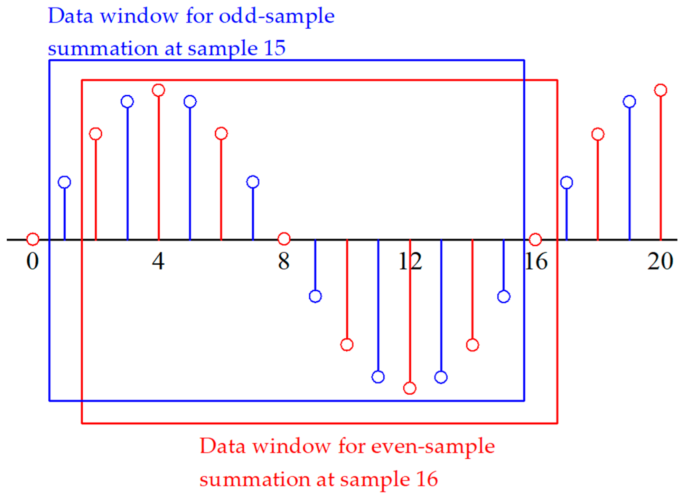
2.1. Dual Decaying DC Offset Estimation

The primary fault current signal in the continuous time domain $i\left(t\right)$ can be expressed as (1):

$$i\left(t\right)={\sum }_{m=1}^{\infty }{A}_m\mathit{sin}\left(\omega t+{\theta }_m\right)+B{e}^{-\frac{t}{\tau }},$$

(1)

where $A_m$ and ${\theta }_m$ are the magnitude and phase angle of the m^th harmonic, respectively. B and $\tau$ are the magnitude and time constant of the DDCO.

By applying the first-order LPF with time constant ${\tau }_{LPF}$ on primary fault current, the output signal of LPF (1) is given in (2).

$$y\left(\mathrm{t}\right)={\sum }_{m=1}^{\infty }{C}_m\mathit{sin}\left(\omega t+{\varphi }_m\right)+A_0{e}^{-\frac{t}{\tau }}+B_0{e}^{-\frac{t}{{\tau }_{LPF}}},$$

(2)

where $C_m$ and ${\varphi }_m$ are the magnitude and phase angle of the m^th harmonic after filtering. $A_0$, $B_0$ are the magnitude of the primary and secondary DDCOs after filtering. Discretizing $y\left(t\right)$ every $∆\mathrm{t}=\frac{2\mathsf{\pi }}{\mathsf{\omega }\times \mathrm{N}}$ becomes, as given in [27]:

$$Y\left[k\right]=A_o{r}^k+B_o{\alpha }^k+{\sum }_{m=1}^{\frac{N}{2}-1}{C}_m\mathit{sin}\left(\frac{2\pi k}{N}m+{\varphi }_m\right),$$

(3)

where $r=e^{-\frac{∆t}{\tau }}$ and $\alpha =e^{-\frac{∆t}{{\tau }_{LPF}}}$ represent the primary and secondary DDCOs, respectively. $Y$ is the current in the discrete time domain. $∆t$ and N are the sampling interval and the number of samples per cycle, respectively.

In this paper, $S$ is defined as the odd- or even-sample summations over N. For example, for a waveform of 16 samples per cycle in Figure 1, $S[15]$ is the sum of the blue samples (1, 3,∙∙∙, 15) and $S[16]$ is the sum of the red samples (2, 4,∙∙∙, 16).

At the sample $k-2$, $k-1$, and $k$, where $k\ge N+1$, the summations can be expressed as (4), (5), and (6), respectively.

$$S\left[k-2\right]={\sum }_{i=1}^{\frac{N}{2}}Y[\left(2i-N\right)+k-2],$$

(4)

$$S\left[k-1\right]={\sum }_{i=1}^{\frac{N}{2}}Y[\left(2i-N\right)+k-1],$$

(5)

$$S\left[k\right]={\sum }_{i=1}^{\frac{N}{2}}Y[\left(2i-N\right)+k],$$

(6)

Substituting (3) into (4) yields:

$$S[k-2]=\sum _{i=1}^{\frac{N}{2}}{A}_o{r}^{\left(2i-N\right)+k-2}+\sum _{i=1}^{\frac{N}{2}}{B}_o{\alpha }^{\left(2i-N\right)+k-2}+\sum _{i=1}^{\frac{N}{2}}\sum _{m=1}^{\frac{N}{2}-1}{A}_m\mathit{sin}\left(\frac{2\pi [\left(2i-N\right)+k-2]}{N}m+{\varphi }_m\right)$$

(7)

Given the following trigonometric relationship:

$${\sum }_{i=1}^{N/2}{\sum }_{m=1}^{\frac{N}{2}-1}{A}_m\sin \left(\frac{2\pi [\left(2i-N\right)+k-2]}{N}m+{\varphi }_m\right)=0,$$

(8)

Only the summation of the dual DDCOs remains in (7). Additionally, using a geometric series, $S[k-2]$, $S[k-1]$, and $S\left[k\right]$ can be simplified to:

$$S[k-2]=A_o\frac{r^{k-N}(r^N-1)}{r^2-1}+B_o\frac{{\alpha }^{k-N}({\alpha }^N-1)}{{\alpha }^2-1},$$

(9)

$$S[k-1]=A_o\frac{r^{1+k-N}(r^N-1)}{r^2-1}+B_o\frac{{\alpha }^{1+k-N}({\alpha }^N-1)}{{\alpha }^2-1},$$

(10)

$$S[k]=A_o\frac{r^{2+k-N}(r^N-1)}{r^2-1}+B_o\frac{{\alpha }^{2+k-N}({\alpha }^N-1)}{{\alpha }^2-1}$$

(11)

Assuming that parameters $X$ and $Y$ are:

$$X=A_o\frac{r^{k-N-1}(r^N-1)}{r^2-1},$$

(12)

$$Y=B_o\frac{{{\alpha }^{k-N-1}(\alpha }^N-1)}{{\alpha }^2-1},$$

(13)

Substituting (12) and (13) into (9), (10), and (11) yield:

$$S[k-2]=rX+\alpha Y,$$

(14)

$$S[k-1]=r^{2}X+{\alpha }^{2}Y,$$

(15)

$$S[k]=r^{3}X+{\alpha }^{3}Y,$$

(16)

As α can be computed from ${\tau }_{LPF}$, a predefined parameter, the systems of (14), (15), and (16) can be solved and $r$, $X$, and $Y$ can be written as:

$$r=\frac{S[k]-\alpha \mathrm{S}[\mathrm{k}-1]}{S[k-1]-\alpha \mathrm{S}[\mathrm{k}-2]}$$

(17)

$$X=\frac{\mathrm{S}[\mathrm{k}-1]-\alpha \mathrm{S}[\mathrm{k}-2]}{r^2-\alpha r}$$

(18)

$$Y=\frac{S[k-2]-rX}{\alpha }$$

(19)

Finally, the magnitude of primary and secondary DDCOs can be estimated using (20) and (21), respectively.

$$A_o=\frac{X(r^2-1)}{r^{k-N-1}(r^N-1)}$$

(20)

$$B_o=\frac{y({\alpha }^2-1)}{{\alpha }^{k-N-1}({\alpha }^N-1)}$$

(21)

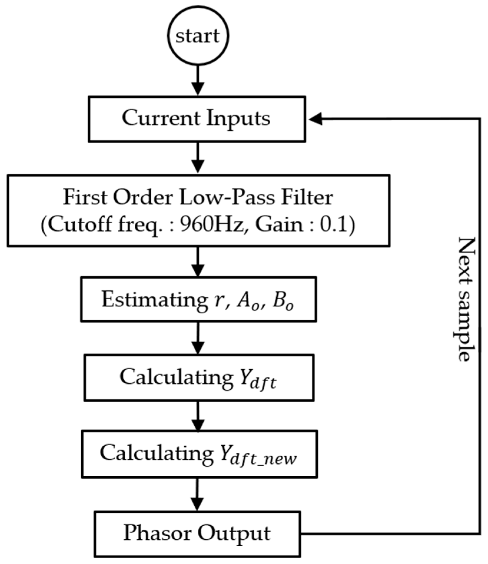
2.2. Enhanced DFT-Based Phasor Estimation

Instead of calculating DDCOs and subtracting them from individual samples, the proposed method involves computing the phasor of the original signal using DFT and subsequently removing fluctuations induced by both primary and secondary DDCOs. The phasor of the original signal $Y_{dft}[k]$ can be obtained by applying the DFT:

$$Y_{dft}[k]=\frac{2}{N}\sum _{i=1}^N\mathrm{Y}[\mathrm{k}-\mathrm{N}+\mathrm{i}]·e^{-\frac{j2\pi (i-1)}{N}}$$

(22)

Substitution of (3) into (22) yields:

$$Y_{dft}[k]=\frac{2}{N}\frac{A_0{r}^{k-N+1}\left(1-r^N\right)}{1-r·e^{-\frac{j2\pi }{N}}}+\begin{array}{c}\frac{2}{N}\frac{B_0{\alpha }^{k-N+1}\left(1-r^N\right)}{1-\alpha ·e^{-\frac{j2\pi }{N}}}+\end{array}\frac{2}{N}\sum _{i=1}^N{C}_m\mathit{sin}\left(\frac{2\pi (k-N+i)}{N}+{\varphi }_1\right)·e^{-\frac{j2\pi (i-1)}{N}}$$

(23)

Finally, the phasor of the fundamental frequency component can be written as:

$$Y_{dft\_new}\left[k\right]=Y_{dft}[k]-\frac{2}{N}\frac{A_0{r}^{k-N+1}\left(1-r^N\right)}{1-r·e^{-\frac{j2\pi }{N}}}-\begin{array}{c}\frac{2}{N}\frac{B_0{\alpha }^{k-N+1}\left(1-r^N\right)}{1-\alpha ·e^{-\frac{j2\pi }{N}}}\end{array}$$

(24)

The real and imaginary parts of (24) can be expressed as:

$$\begin{array}{ll}{Y}_{dft\_new}^{re}\left[k\right]=& \frac{2}{N}\left(\sum _{i=1}^N\mathrm{Y}[k-N+i]·\cos \left(2\pi \left(i-1\right)\right)\right)-\frac{2}{N}\times \frac{A_0{r}^{k-N+1}\left(1-r^N\right)}{\left(1-2r·\mathit{cos}\left(\frac{2\pi }{N}\right)+r^2\right)}\left(1-r·cos\left(\frac{2\pi }{N}\right)\right)\\ & -\frac{2}{N}\times \frac{B_0{\alpha }^{k-N+1}(1-{\alpha }^N)}{\left(1-2\alpha ·\mathit{cos}\left(\frac{2\pi }{N}\right)+{\alpha }^2\right)}\left(1-\alpha ·cos\left(\frac{2\pi }{N}\right)\right)\end{array}$$

(25)

$$\begin{array}{ll}{Y}_{dft\_new}^{im}\left[k\right]=& -\frac{2}{N}\left(\sum _{i=1}^N\mathrm{Y}[k-N+i]·\sin \left(2\pi \left(i-1\right)\right)\right)-\frac{2}{N}\times \frac{A_0{r}^{k-N+1}(1-r^N)}{\left(1-2r·\mathit{cos}\left(\frac{2\pi }{N}\right)+r^2\right)}\left(-r·sin\left(\frac{2\pi }{N}\right)\right)\\ & -\begin{array}{c}\frac{2}{N}\times \frac{B_0{\alpha }^{k-N+1}(1-{\alpha }^N)}{\left(1-2\alpha ·\mathit{cos}\left(\frac{2\pi }{N}\right)+{\alpha }^2\right)}\left(-\alpha ·sin\left(\frac{2\pi }{N}\right)\right)\end{array}\end{array}$$

(26)

where $Y_{dft}$ and $Y_{dft\_new}$ represent the phasor estimation of the original DFT and the enhanced DFT, respectively. $Y_{dft\_new}^{re}$ and $Y_{dft\_new}^{im}$ are the real and imaginary parts of the enhanced DFT-based phasor estimation, while $j$ denotes the complex operator. Figure 2 shows the flowchart of the enhanced DFT-based phasor estimation.

3. Performance Evaluation

To demonstrate the efficacy of the proposed method, mathematically generated and PSCAD/EMTDC-generated signals are used in this paper. To evaluate superiority over the recent methods, the new proposed method is compared with the conventional DFT, MDFT 2022 [24], and MDFT 2023 [26]. The signal is pre-conditioned by a first-order LPF which exhibits a gain of 0.1 at a cutoff frequency of 960 Hz [10]. The sampling frequency is 3840 Hz (64 samples per cycle in 60 Hz system).

3.1. Mathematically Generated Signal

3.1.1. Normal Conditions

In scenario 1, the power system is assumed to be operating in normal conditions. The current signal is a sinewave represented by:

$$Y[k]=100\mathit{sin}\left(\frac{2\pi k}{64}\right)$$

(27)

Figure 3 shows the phasor estimation of each method employed on the signal generated by (27). Among the three methods, MDFT 2022 exhibited the fastest convergence, whereas MDFT 2023 presented the slowest convergence speed. The new proposed method converges faster (N − 1 = 63) than the theoretical convergence time (N + 1 = 65).

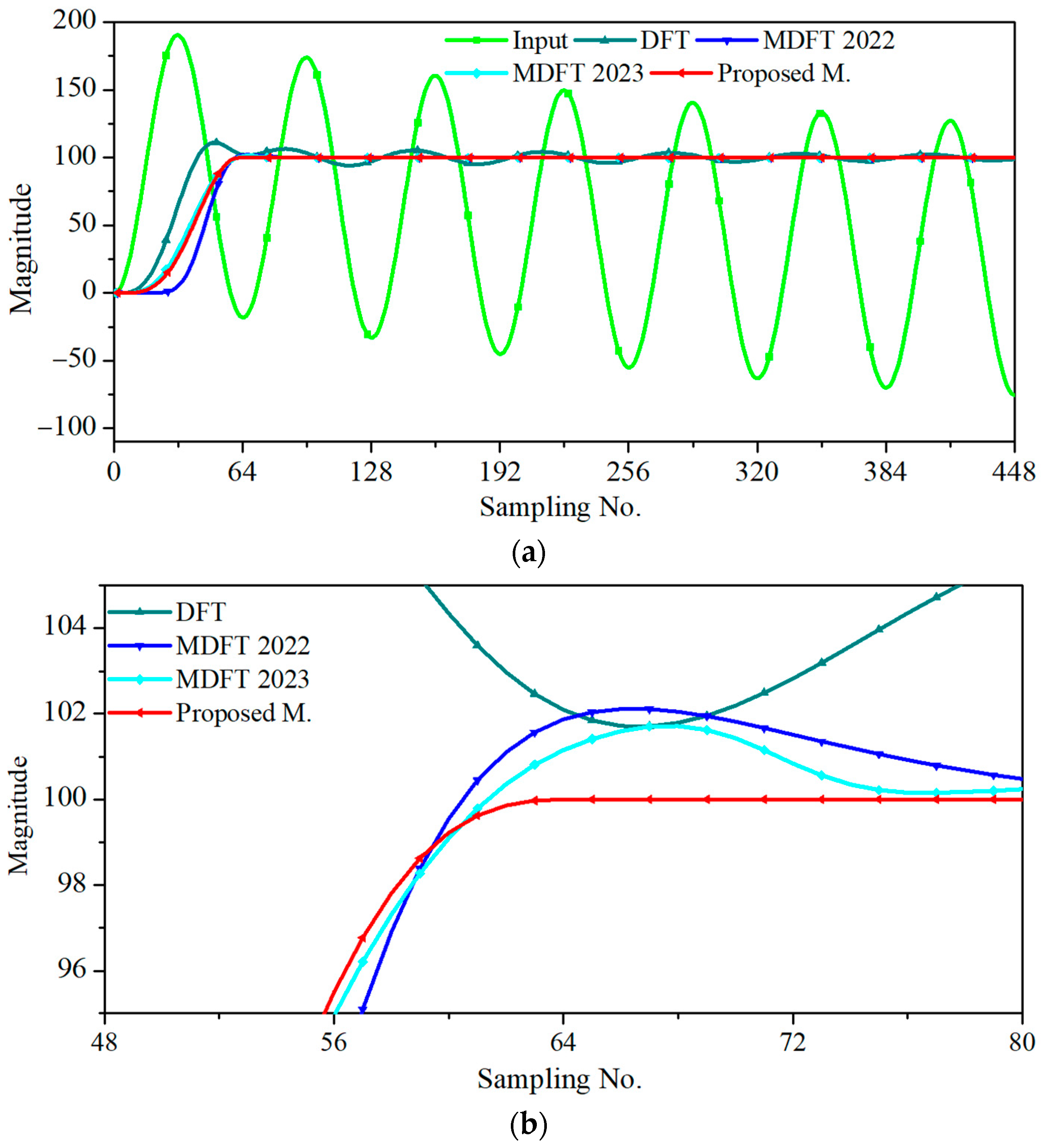
3.1.2. Input Signal Containing a Primary DDCO with a Time Constant of Half Cycle

In scenario 2, the focus is on the primary DDCO that contains a half-cycle time constant:

$$Y[k]=100\mathit{sin}\left(\frac{2\pi k}{64}+\frac{3\pi }{2}\right)+100e^{-\frac{k}{\left(60\times 64\right)\times 1/60\times 0.5}}$$

(28)

Figure 4 shows the phasor estimation of the input signal containing the time constant of the half cycle generated from (28). The conventional DFT yielded larger errors than the other methods. Figure 4b shows that MDFT 2022 and MDFT 2023 could not converge at sample N + 1, but the proposed method converged after sample N. Assuming an accuracy requirement of ±1%, the new proposed method was more promising in terms of convergence speed and accuracy.

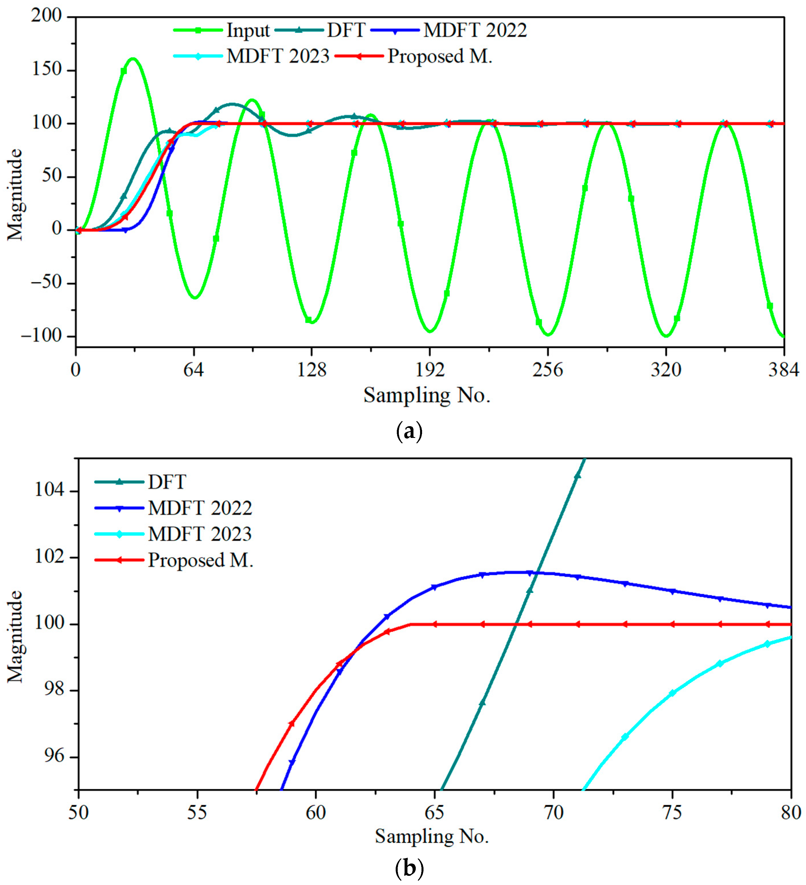
3.1.3. Input Signal Containing a Primary DDCO with a Time Constant of 5 Cycles

Scenario 3 represents a case in which the primary DDCO has a time constant of 5 cycles (i.e., a long time constant):

$$Y[k]=100\mathit{sin}\left(\frac{2\pi k}{64}+\frac{3\pi }{2}\right)+100e^{-\frac{k}{\left(60\times 64\right)\times 1/60\times 5.0}}$$

(29)

As shown in Figure 5, the proposed method converged to within ±1% error after sample N. However, MDFT 2022 and MDFT 2023 only converged at samples N + 12 (=76) and N + 8 (=72), respectively.

The scenarios showed the following results:

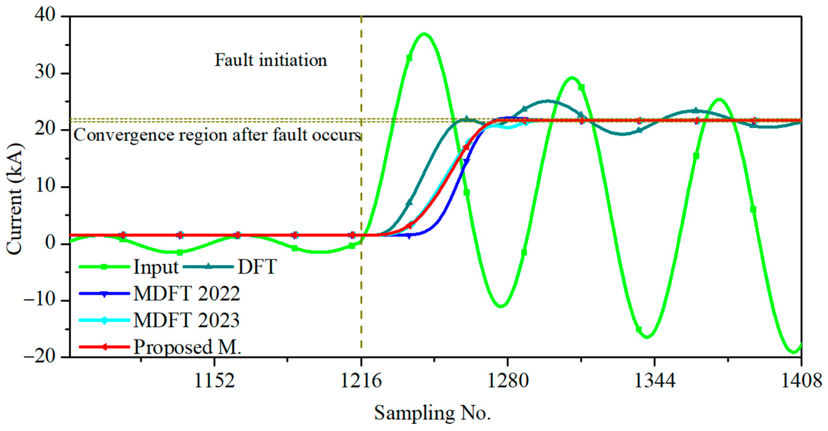
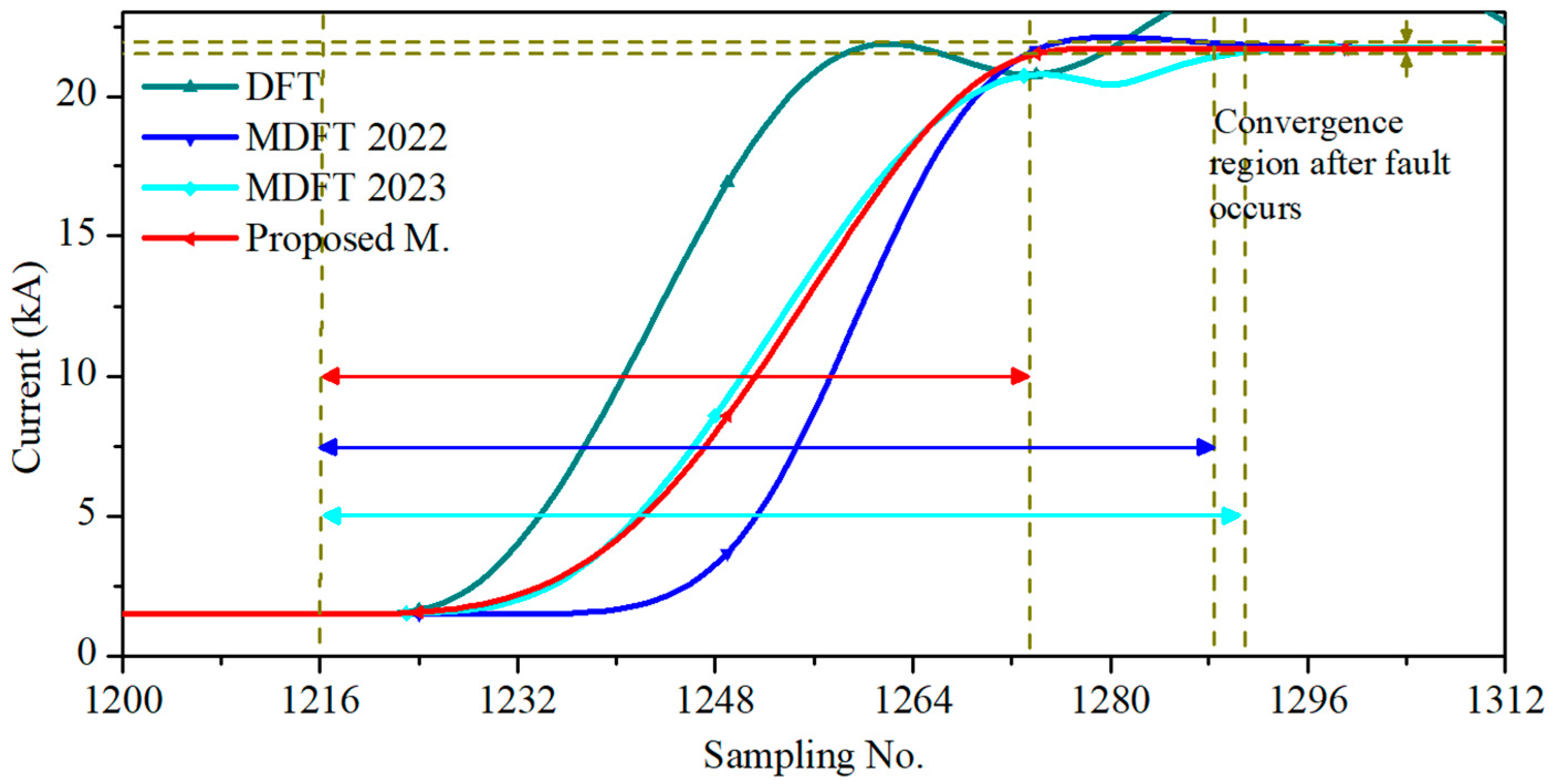
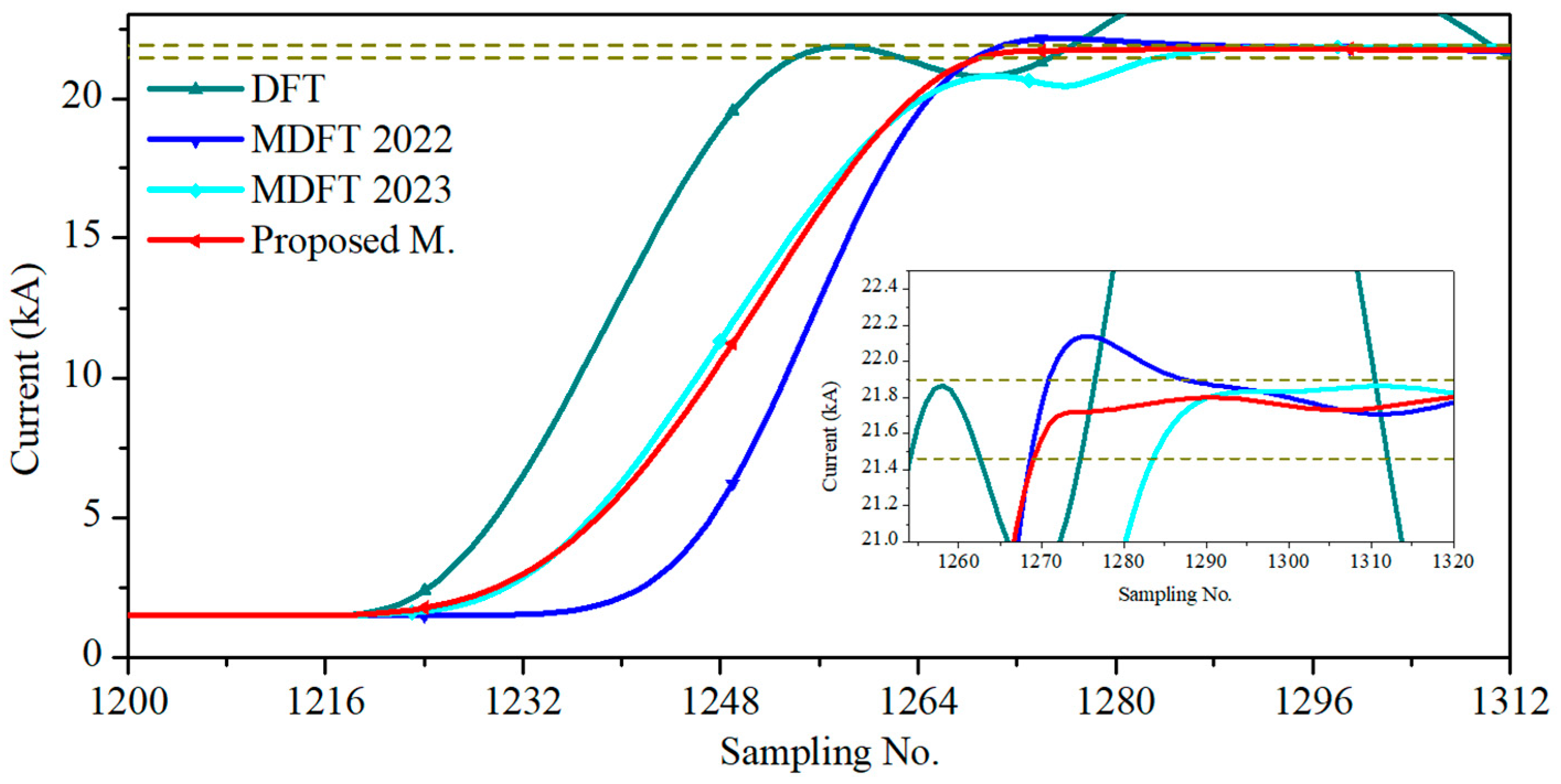
• Conventional DFT clearly presented the worst performance when dual DDCOs were present. In certain cases, the maximum error exceeded 20% and the convergence time to an error accuracy of ±5% reached 3 cycles;
• MDFT 2022 was negatively affected when the primary DDCO had a large time constant, but worked well under normal conditions or when the primary DDCO exhibited a small time constant;
• MDFT 2023 performed very poorly when the primary DDCO exhibited a small time constant;
• The new proposed DFT-based phasor estimation method converged within N samples without any error because approximation was not needed;
• If an accuracy of ± 1% is required, the proposed method is optimal in all scenarios.

3.2. PSCAD/EMTDC-Generated Signal

The performance of the proposed method was evaluated for phase a-to-ground faults (a–g faults) on a 154 kV 26 km overhead transmission line as illustrated in Figure 6. $E_S$ and $Z_S$ represent the voltage and impedance of the sending end, while $E_R$ and $Z_R$ represent the voltage and impedance of the receiving end. The magnitudes of E_R and E_S were 154 kV with phase angles of 20° and 5°, respectively. $Z_S$ is 0.1921 + j2.0538 [Ω], and $Z_R$ is 0.5478 + j3.7187 [Ω]. A current transformer (CT) was used to measure the fault current seen by the source. The line parameters are provided in

Table 1. The 154 kV transmission line parameters.

Sequence	Parameter	Value	Unit
Positive and Negative	$R_1$$,R_2$	0.0419	Ω/km
	$L_1$$,L_2$	0.8921	mH/km
	$C_1$$,C_2$	0.0128	µF/km
Zero	$R_0$	0.0293	Ω/km
	$L_0$	2.6657	mH/km
	$C_0$	0.0042	µF/km

. Line resistance, line inductance, and line capacitance are denoted as $R$, $L$, and $C$, respectively, while subscripts 1 and 2 indicate positive and negative sequence. Zero-sequence line parameters such as resistance, inductance, and capacitance are denoted as $R_0$, $L_0$, and $C_0$, respectively. PSCAD/EMTDC was used to generate fault current signals in different fault distances varying from 5 to 13 km and fault inception angles were covered from 0 to 90°.The sampling frequency was set to 3840 Hz (64 samples per cycle in 60 Hz systems).

Figure 7 shows the phasor estimation of an a–g fault current at a distance of 5 km from the sending end source and inception angle of 0°. The proposed method was compared with other methods based on the convergence region within ±1%. The conventional DFT exhibited fluctuations for several cycles until DDCO disappeared. MDFT 2022 and MDFT 2023 failed to reach the convergence region before sample N. The proposed method showed a faster response than the conventional method and MDFT methods, as it settled in the convergence region earlier than sample N.

The maximum errors produced by the newly proposed DFT-based method after sample N from fault initiation are summarized in

Table 2. Maximum errors after the 64th sample after fault initiation.

Fault Distance	Fault Inception Angle	MDFT 2022	MDFT 2023	Proposed Method
5 (km)	0°	1.77%	6.00%	0.17%
	30°	0.14%	0.48%	0.14%
	60°	3.55%	3.70%	0.55%
	90°	5.79%	1.08%	1.08%
10 (km)	0°	1.79%	7.22%	0.19%
	30°	0.25%	0.65%	0.15%
	60°	3.43%	3.58%	0.24%
	90°	5.49%	1.28%	0.87%
13 (km)	0°	1.81%	7.32%	0.22%
	30°	0.29%	0.90%	0.17%
	60°	3.37%	3.48%	0.16%
	90°	4.81%	1.25%	0.67%

; the estimation errors were within the acceptable range. The best performance of MDFT 2022 was achieved at a fault distance of 5 km and fault inception angle of 30°. Table 2 also shows that the estimation error of MDFT 2022 was between 0.14% and 5.79%. Unlike MDFT 2022, MDFT 2023 presented more errors as the fault distance increased and the fault inception angle was small; the maximum error yielded was 7.32% at a fault inception angle of 0° and a distance of 13 km away from the measured point. It is noted that the MDFT 2023 results are dissatisfactory in terms of the maximum error produced by all cases compared to MDFT 2022. However, at a fault inception angle of 90°, MDFT 2023 provided a better result than MDFT 2022 at all fault distances (5 km, 10 km, and 13 km). On the other hand, the proposed method demonstrated the worst maximum error of 1.08% when the fault occurred at a fault inception angle of 90° and a distance of 5 km. In addition to this, the performance evaluation based on the maximum errors demonstrated in Table 2 shows that the maximum error of the proposed method is generally lower than 1%, which implies the strong capability of the proposed method in estimating DDCOs even when dual DDCOs are present. Table 2 also demonstrates the low maximum errors of all methods where the fault inception angle is 30° at any fault distance. These results are caused by the transmission configuration and the utilized low-pass filter.

The convergence time served as an evaluation index; this is the time required for the estimated amplitude to remain within 1% of the actual value from the fault initiation. Figure 8 shows the convergence time of MDFT 2022, MDFT 2023, and the new proposed method in milliseconds. It is apparent that the convergence time of the proposed method reached the steady-state region quicker than MDFT 2022 and MDFT 2023.

Table 3. Summary of convergence times.

Fault Distance	Fault Inception Angle	MDFT 2022	MDFT 2023	Proposed Method
5 (km)	0°	18.75 ms	19.27 ms	15.10 ms
	30°	14.06 ms	16.66 ms	15.88 ms
	60°	18.75 ms	18.22 ms	16.40 ms
	90°	18.75 ms	16.92 ms	16.92 ms
10 (km)	0°	18.75 ms	19.53 ms	15.36 ms
	30°	14.06 ms	16.66 ms	15.88 ms
	60°	18.75 ms	18.22 ms	16.40 ms
	90°	18.75 ms	17.44 ms	16.40 ms
13 (km)	0°	18.75 ms	19.53 ms	15.36 ms
	30°	14.06 ms	16.66 ms	15.88 ms
	60°	18.75 ms	18.22 ms	16.40 ms
	90°	18.48 ms	16.92 ms	16.40 ms

summarizes the convergence time at various fault distances and fault inception angles. The best convergence times achieved by MDFT 2022 and MDFT 2023 were 14.06 ms and 16.66 ms, respectively. Considering the worst scenario, MDFT 2023 displayed a maximum convergence time of 19.53 ms. Unlike MDFTs, the proposed method rapidly converged compared to the other methods; the worst convergence time was 16.92 ms (corresponding to 65 samples), and convergence was usually achieved within 64 samples.

3.3. Off-Nominal Frequency Operation

Assuming the system frequency to be constant, the source frequency in the simulations was changed from 60 to 60.2 Hz to consider off-nominal frequency operation. Figure 9 shows the phasor estimation of an a-g fault current at a distance of 5 km and fault inception angle of 0°. The proposed method, MDFT 2022, and MDFT 2023 all adequately managed off-nominal frequency operation; the phasors were accurately estimated. The proposed method converged at 14.06 ms; MDFT 2022 and MDFT 2023 converged at 18.75 ms and 17.70 ms, respectively. The maximum error of the proposed method was 0.62% after sample N from fault inception.

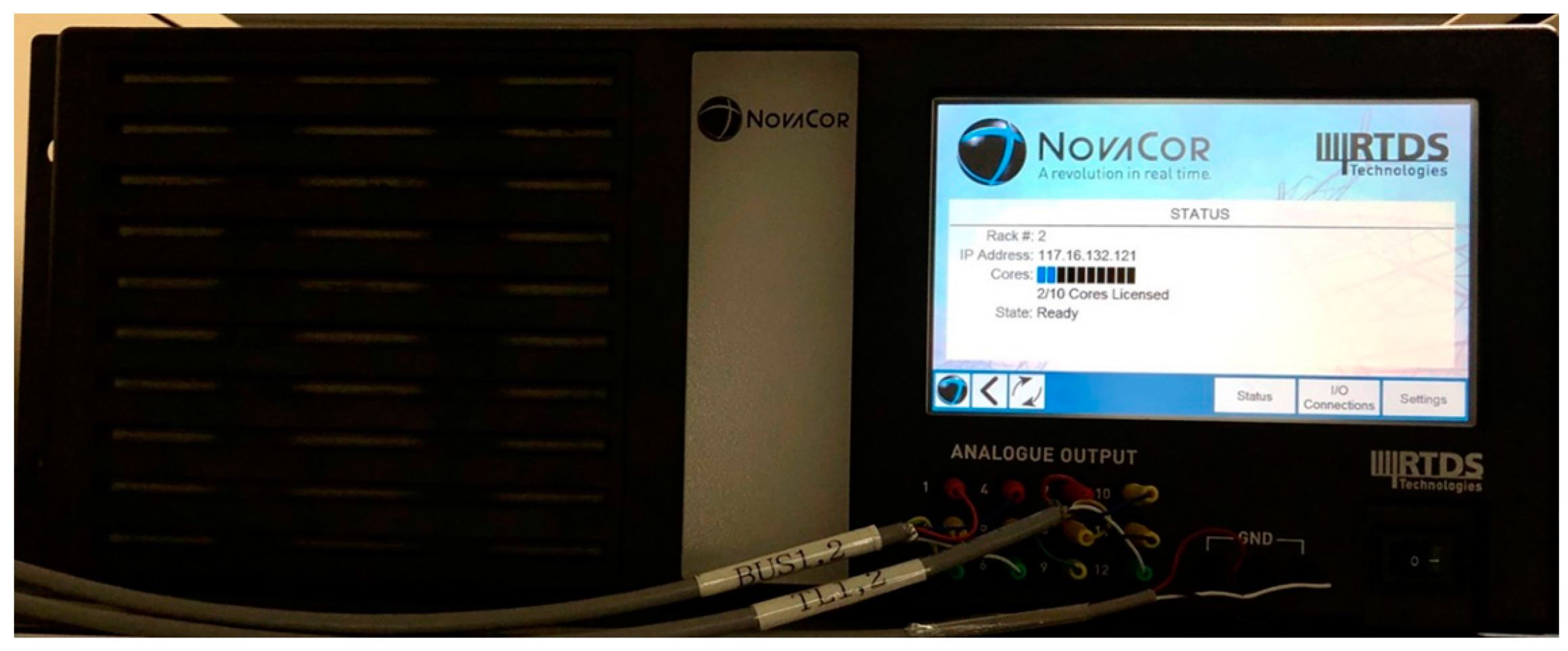
4. Hardware Prototype and Results

The proposed enhanced DFT-based phasor estimation was implemented in a prototype composed of a TI ADS86xx EVM and a TI AM574x IDK. The hardware was tested using the system configuration shown in Figure 10.

An RTDS module as shown in Figure 11 was used to generate analog signals. Similarly, the power system configuration in PSCAD/EMTDC was used to model in RSCAD. Analog signals were converted to digital signals using the TI ADS86xx EVM as shown in Figure 12a, operating at 3840 Hz. All digital signals were then processed by the TI AM574x IDK depicted in Figure 12b.

The phasor estimations of an a–g fault current at a distance of 5.2 km are shown in Figure 13a,b for fault inception angles of 0° and 90°, respectively. The time responses in the hardware tests were nearly identical to the responses in simulation tests, reaching a steady state at approximately 15.62 ms (corresponding to 60 samples) and 16.92 ms (corresponding to 65 samples) for fault inception angles of 0° and 90°, respectively. However, due to the effects of ADC and noise, the hardware test errors were slightly greater with maximum error values of 0.86% and 1.26% for fault inception angles of 0° and 90°, respectively. Therefore, it was found that the prototype accurately estimated the phasor of the fault current signal in real time within sample N + 1, as proposed by this method.

5. Conclusions

We present a novel method for the removal of dual DDCOs to enhance DFT phasor estimation. The proposed method estimates the magnitudes of the first and second DDCOs, and the time constant of the first DDCO. Then, the phasor containing no DC component is obtained by subtracting fluctuations from the phasor of the input signal using the estimated parameters of the DDCOs. The performance of the proposed method was compared with those of two recent methods (MDFT 2022 and MDFT 2023). Simulations using mathematically generated signals and PSCAD/EMTDC-generated signals showed that the proposed method was more accurate and quicker than the other methods, regardless of variations in the primary DDCO. The effect of dual DDCOs does not impact the performance of the proposed method considering different time constants. Hardware implementation was conducted to confirm that the new method can be applied to existing devices. The method is considered a practical solution for real-time protection due to its low computational burden, in addition to accuracy and convergence speed.

As future work, the phasor estimation algorithms should be improved to perform correct estimations while using fewer samples with higher accuracy and robustness against any harmonics and noises. Dynamic frequency variation should be considered since variable renewable energy is increasing annually. Moreover, other real filters used in power system protection should be studied to effectively eliminate the effects of DDCOs in phasor estimation.

References

1. Yu, S.L.; Gu, J.C. Removal of decaying DC in current and voltage signals using a modified Fourier filter algorithm. IEEE Trans. Power Deliv. 2001, 16, 372–379. [Google Scholar]
2. Gu, J.C.; Yu, S.L. Removal of DC offset in current and voltage signals using a novel Fourier filter algorithm. IEEE Trans. Power Deliv. 2000, 15, 73–79. [Google Scholar]
3. Mohammadi, S.; Mahmoudi, A.; Kahourzade, S.; Yazdani, A.; Shafiullah, G. Decaying DC Offset Current Mitigation in Phasor Estimation Applications: A Review. Energies 2022, 15, 5260. [Google Scholar] [CrossRef]
4. Girgis, A.A. A new kalman filtering based digital distance relay. IEEE Trans. Power Appar. Syst. 1982, 101, 3471–3480. [Google Scholar] [CrossRef]
5. Benmouyal, G. Frequency-doman characterization of kalman filters as applied to power system protection. IEEE Trans. Power Del. 1992, 7, 1129–1138. [Google Scholar] [CrossRef]
6. Benmouyal, G. Removal of DC-offset in current waveforms using digital mimic filtering. IEEE Trans. Power Deliv. 1995, 10, 621–630. [Google Scholar] [CrossRef]
7. Sachdev, M.; Baribeau, M. A new algorithm for digital impedance relays. IEEE Trans. Power Appar. Syst. 1979, 98, 2232–2240. [Google Scholar] [CrossRef]
8. Isaksson, A. Digital protective relaying through recursive least-squares identification. Proc. Inst. Elect. Eng. Gen. Transm. Distrib. 1988, 135, 441–449. [Google Scholar] [CrossRef]
9. Sachdev, M.; Nagpal, M. A recursive least error squares algorithm for power system relaying and measurement applications. IEEE Trans. Power Deliv. 1991, 6, 1008–1015. [Google Scholar] [CrossRef]
10. Jafarian, P.; Sanaye-Pasand, M. An adaptive phasor estimation technique based on LES method using forgetting factor. In Proceedings of the 2009 IEEE Power and Energy Society General Meeting (PES ′09), Calgary, AB, Canada, 26–30 July 2009; pp. 1–8. [Google Scholar]
11. Jafarian, P.; Sanaye-Pasand, M. Weighted least error squares based variable window phasor estimator for distance relaying application. IET Gener. Transm. Distrib. 2011, 5, 298–306. [Google Scholar] [CrossRef]
12. Hwang, J.K. Least error squared phasor estimation with identification of a decaying DC component. IET Gener. Transm. Distrib. 2018, 12, 1486–1492. [Google Scholar] [CrossRef]
13. Min, K.W.; Santoso, S. DC offset removal algorithm for improving location estimates of momentary faults. IEEE Trans. Smart Grid 2018, 9, 5503–5511. [Google Scholar] [CrossRef]
14. Achlerkar, P.D.; Panigrahi, B.K. Assessment of DC offset in fault current signal for accurate phasor estimation considering current transformer response. IET Sci. Meas. Technol. 2019, 13, 403–408. [Google Scholar] [CrossRef]
15. da Silva, C.D.L.; Cardoso, G.; de Morais, A.P.; Marchesan, G.; Guarda, F.G.K. A continually online trained impedance estimation algorithm for transmission line distance protection tolerant to system frequency deviation. Electr. Power Syst. Res. 2017, 147, 73–80. [Google Scholar] [CrossRef]
16. Kim, S.-B.; Sok, V.; Kang, S.-H.; Lee, N.-H.; Nam, S.-R. A Study on Deep Neural Network-Based DC Offset Removal for Phase Estimation in Power Systems. Energies 2019, 12, 1619. [Google Scholar] [CrossRef]
17. Sok, V.; Lee, S.-W.; Kang, S.-H.; Nam, S.-R. Deep Neural Network-Based Removal of a Decaying DC Offset in Less Than One Cycle for Digital Relaying. Energies 2022, 15, 2644. [Google Scholar] [CrossRef]
18. Nam, S.-R.; Kang, S.-H.; Park, J.-K. An analytic method for measuring accurate fundamental frequency components. IEEE Trans. Power Deliv. 2002, 17, 405–411. [Google Scholar] [CrossRef]
19. Nam, S.-R.; Kang, S.-H.; Sohn, J.-M.; Park, J.-K. Modified notch filter-based instantaneous phasor estimation for high-speed distance protection. Electr. Eng. 2007, 89, 311–317. [Google Scholar] [CrossRef]
20. Rao, J.T.; Bhalja, B.R.; Andreev, M.V.; Malik, O.P. Synchrophasor Assisted Power Swing Detection Scheme for Wind Integrated Transmission Network. IEEE Trans. Power Deliv. 2022, 37, 1952–1962. [Google Scholar] [CrossRef]
21. Kumar, P.; Kumar, V.; Tyagi, B. Islanding detection for reconfigurable microgrid with RES. IET Gener. Transm. Distrib. 2021, 15, 1187–1202. [Google Scholar] [CrossRef]
22. Rao, J.T.; Bhalja, B. A New Phase Angle of Superimposed Positive Sequence Current-Based Discrimination Scheme for Prevention of Maloperation of Distance Relay During Severe Stressed Conditions. IEEE Syst. J. 2020, 14, 3705–3716. [Google Scholar] [CrossRef]
23. Mohammadi, S.; Rezaei, N.; Mahmoudi, A. A novel analytical method for DC offset mitigation enhancing DFT phasor estimation. Electr. Power Syst. Res. 2022, 209, 108036. [Google Scholar] [CrossRef]
24. Yu, H.; Jin, Z.; Zhang, H.; Terzija, V. A Phasor Estimation Algorithm Robust to Decaying DC Component. IEEE Trans. Power Deliv. 2022, 37, 860–870. [Google Scholar] [CrossRef]
25. Afrandideh, S.; Haghjoo, F. A DFT-based phasor estimation method robust to primary and secondary decaying DC components. Electr. Power Syst. Res. 2022, 208, 107907. [Google Scholar] [CrossRef]
26. Afrandideh, S. A Modified DFT-Based Phasor Estimation Algorithm Using an FIR Notch Filter. IEEE Trans. Power Deliv. 2023, 38, 1308–1315. [Google Scholar] [CrossRef]
27. Yong Guo, M. Kezunovic and Deshu Chen. Simplified algorithms for removal of the effect of exponentially decaying DC-offset on the Fourier algorithm. IEEE Trans. Power Deliv. 2003, 18, 711–717. [Google Scholar] [CrossRef]
Figure 1. Data windows for odd- and even-sample summations at sample 15 and sample 16, respectively (N = 16).
Energies 17 00905 g001
Figure 2. Flowchart of the enhanced DFT-based phasor estimation.
Energies 17 00905 g002
Figure 3. Phasor estimations under normal conditions: (a) Phasor magnitudes. (b) Close-up of the convergences.
Energies 17 00905 g003
Figure 4. Phasor estimations when the input signal contained a primary DDCO with a half-cycle time constant: (a) Phasor magnitudes. (b) Close-up of the convergences.
Energies 17 00905 g004
Figure 5. Phasor estimations when the input signal contains a primary DDCO with a time constant of 5 cycles. (a) Phasor magnitudes. (b) Close-up of the convergences.
Energies 17 00905 g005
Figure 6. Single-line diagram of 154 kV Korean overhead transmission system.
Energies 17 00905 g006
Figure 7. Phasor estimation of an a-g fault current at a distance of 5 km and inception angle of 0°.
Energies 17 00905 g007
Figure 8. Convergence times of the new method, MDFT 2022, and MDFT 2023.
Energies 17 00905 g008
Figure 9. Phasors of an a-g fault current at a distance of 5 km and inception angle of 0° in an off-nominal frequency scenario.
Energies 17 00905 g009
Figure 10. Block diagram of hardware implementation.
Energies 17 00905 g010
Figure 11. Generation of analog signals by the RTDS.
Energies 17 00905 g011
Figure 12. Hardware prototype: (a) TI ADS86xx EVM. (b) TI AM574x IDK.
Energies 17 00905 g012
Figure 13. Phasors estimated by the hardware prototype for an a-g fault current at a distance of 5.2 km: (a) Inception angle of 0°. (b) Inception angle of 90°.
Energies 17 00905 g013