Abstract
Dynamic economic emission dispatch problems are complex optimization tasks in power systems that aim to simultaneously minimize both fuel costs and pollutant emissions while satisfying various system constraints. Traditional methods often involve solving intricate nonlinear load flow equations or employing approximate loss formulas to account for transmission losses. These methods can be computationally expensive and may not accurately represent the actual transmission losses, affecting the overall optimization results. To address these limitations, this study proposes a novel approach that integrates transmission loss prediction into the dynamic economic emission dispatch (DEED) problem. A Random Forest machine learning model was offline-trained to predict transmission losses accurately, eliminating the need for repeated calculations during each iteration of the optimization process. This significantly reduced the computational burden of the algorithm and improved its efficiency. The proposed method utilizes a powerful multi-objective stochastic paint optimizer to solve the highly constrained and complex dynamic economic emission dispatch problem integrated with random forest-based loss prediction. A fuzzy membership-based approach was employed to determine the best compromise Pareto-optimal solution. The proposed algorithm integrated with loss prediction was validated on widely used five and ten-unit power systems with B-loss coefficients. The results obtained using the proposed algorithm were compared with seventeen algorithms available in the literature, demonstrating that the multi-objective stochastic paint optimizer (MOSPO) outperforms most existing algorithms. Notably, for the Institute of Electrical and Electronics Engineers (IEEE) thirty bus system, the proposed algorithm achieves yearly fuel cost savings of USD 37,339.5 and USD 3423.7 compared to the existing group search optimizer algorithm with multiple producers (GSOMP) and multi-objective multi-verse optimization (MOMVO) algorithms.
1. Introduction
Using coal in power stations to produce electricity is inefficient, resulting in greenhouse gases and other harmful gas emissions to the atmosphere [1]. For sustainable development and to meet the stringent regulatory requirements, power plants that produce power using coal or other fossil fuels are forced to reduce air pollution levels and minimize fuel costs. To achieve these requirements, a multi-objective dynamic economic emission dispatch (DEED) model was formulated in the literature to minimize the conflicting objectives of the fuel cost and emission levels. When compared to the combined economic emission dispatch (CEED) problem, a DEED problem is more complicated as it incorporates a time-varying load pattern along with ramp-up and ramp-down limits of the generator. Finding a solution to a DEED problem involves solving nonlinear and non-differentiable equations. Traditional mathematical models that rely on solving derivatives will fail to solve the DEED problem when generator valve-point effects [2] are considered. Traditional methods such as gradient-based optimization, linear programming, and heuristic methods struggle with non-convex or large-scale DEED problems, where finding globally optimal solutions becomes challenging. DEED is a bi-dimensional problem with linear and nonlinear equality and inequality constraints. Finding a non-inferior solution for a specific time horizon in a DEED problem requires a contemporary and robust multi-objective algorithm.
1.1. Solving Multi-Objective DEED Using Single-Objective Algorithm
The particle swarm optimization (PSO) algorithm using the goal attainment method in [3], the evolutionary programming (EP) algorithm [4], and the pattern search (PS) method used in [5] rely on the individual’s knowledge. Variants of the PSO in [6] named standard PSO (SPSO), PSO with avoidance of worst location (PSOAWL), and PSO with gradually increasing directed neighborhood (PSO GIDN), resulted in an improved information exchange between the particles of PSO. However, they considerably increased the complexity of the algorithm. Variants of harmony search, such as NPAHS in [7] and enhanced harmony search in [8], are capable of finding Pareto-optimal (PO) solutions to the DEED problem. The efficient and enhanced differential evolution algorithm in [9] incorporates several local parameters. However, tuning these local parameters is complicated. Normalized objective functions were used in [8,9], along with an efficient strategy for constraint handling to combine two objectives into a single-objective function. The real-coded genetic algorithm in [10] combines multiple conflicting objectives using penalty factors which vary from one test system to another. Hybrid algorithms have also been used to improve the capabilities of the existing algorithms to solve the DEED problem. The hybrid algorithms in [11,12] solve the complicated DEED problem considering periodic and seasonal loads. A single-objective COOT optimization algorithm solves the DEED problem by combining conflicting objectives using weights [13]. An improved mayfly algorithm was employed to solve the CEED problem integrated with renewable energy sources [14].
The main drawback of employing single-objective algorithms to solve a bi-objective DEED problem is that the conflicting objectives must be converted into an equivalent single-objective function using penalty factors or weights. Furthermore, when PO solutions are required, the single-objective algorithm must be run several times by changing the weights during each run. Using a single-objective algorithm to solve a bi-objective DEED problem introduces limitations in terms of Pareto optimality, objective prioritization, solution diversity, and robustness. To address these drawbacks, employing multi-objective optimization techniques specifically designed for bi-objective problems is essential to ensure a more comprehensive exploration of the solution space and to facilitate informed decision-making.
1.2. Solving Multi-Objective DEED Using Multi-Objective Algorithm
The main advantage of using multi-objective algorithms to solve DEED problems is that PO solutions are obtained in a single run. The real-coded genetic algorithm (RCGA) and non-dominated sorting genetic algorithm II (NSGAII) in [15], and its improved version in [16], have been used to obtain non-dominated solutions for a DEED problem in a single run for a ten-unit system. The Pareto dominance-incorporated group search optimizer algorithm with multiple producers (GSOMP) in [17] can successfully solve the DEED problem. A multi-objective version of the single-objective differential evolution algorithm in [18] and its enhanced version in [19] have employed a constraint handling management technique that requires many computations to solve the DEED problem. A multi-objective version of the differential evolution algorithm was hybridized with a simulated annealing algorithm (MODE-SAT) [20] and employed to solve five-unit and ten-unit systems. To reduce the computational burden in solving the DEED problem, a multi-objective proximal policy optimization (MOPPO) algorithm was used in [21] along with the Markov decision process, where most of the computations were transferred to offline. Furthermore, a trained artificial neural network (ANN) and an improved fitness function were incorporated in [22] to solve the DEED problem. The drawbacks of the methods proposed in [21,22] are that they require many hyperparameters to be tuned, and the PO solutions obtained are inferior to many existing algorithms. A multi-objective salp swarm algorithm was employed in [23] to obtain the PO solutions for 6-unit, 10-unit, and 14-unit test systems. The best compromise solution was obtained using the fuzzy membership method. Many recent works have also integrated renewable energy sources with DEED [24,25,26].
1.3. Modeling Transmission Loss in DEED Formulation
The two most widely used methods of transmission loss modeling are to use a single B-loss coefficient for the 24 h in a day, as in [3,4,5,6,7,8,9,11,12,15,17,21,22]; or to solve load flow equations, as in [16,18,19,20,27]. Both these models have a significant drawback when applied to the DEED formulation. As load varies from hour to hour, using a single B-loss coefficient for 24 h will result in an inaccurate transmission loss calculation. Solving the complex power flow equations during each iteration to find the power loss dramatically increases the computational efforts, increasing the convergence time. Various other approaches, such as modeling using the quadratic equation in [28], loss prediction using an ANN in [29], and other different methods are investigated in detail in [30]. This research tries to integrate a machine learning-based algorithm to predict the transmission loss without increasing the computational complexity. The literature survey indicates that the random forest algorithm has not been used for transmission loss prediction so far; hence, this research attempts to integrate transmission loss prediction using random forest in the DEED formulation.
2. Contribution
Traditionally, solving DEED problems involved incorporating losses computed using intricate nonlinear load flow equations or by using approximate loss formulas, both of which could be computationally expensive and the loss formula might not precisely capture actual transmission losses. The authors have employed powerful algorithms to solve the various economic dispatch formulations including the DEED problem in [31,32,33,34,35,36,37,38]. The integration of the machine learning model into the DEED problem is not widely explored in the literature. The authors were the first to attempt the integration of ANN into the DEED formulation using multi-objective multi-verse optimization (MOMVO) [29].
Random forest is a powerful machine learning algorithm that has been effective for a variety of prediction tasks. Thus, the innovation in this research lies in the integration of a random forest machine learning model to predict transmission losses and its integration in the dynamic economic emission dispatch (DEED) formulation. While DEED problems are not new and have been tackled using various optimization methods, the introduction of machine learning to accurately predict transmission losses is a novel approach. This is the first attempt to integrate random forest into the DEED formulation that the authors are aware of.
The use of a random forest machine learning model, offline-trained to predict these losses, is a unique and innovative solution. In doing so, the method eliminates the need for repeated calculations of transmission losses during each iteration of the optimization process, significantly reducing the computational burden and improving efficiency. As the transmission loss is predicted only once by the random forest model during a period of dispatch, the proposed method reduces the algorithm’s complexity when compared to employing B-loss coefficients or power flow equations. This integration significantly reduces the computational burden of the DEED problem and improves its efficiency. The novelty of the proposed approach lies in integrating the random forest-based transmission loss prediction into the DEED formulation.
Further, the authors were motivated by the fact provided in [39] that there is always room to create potent algorithms to tackle challenging problems. This fact inspired the authors to utilize a newly developed MOSPO algorithm integrated with random forest to find the Pareto-optimal solution to a very tough and highly challenging DEED problem. The integration of a powerful multi-objective stochastic paint optimizer and a fuzzy membership-based approach to determine the best compromise Pareto-optimal solution further adds to the innovation. These elements collectively contribute to a more effective and efficient solution to the DEED problem compared to existing algorithms in the literature.
3. Dynamic Economic Emission Dispatch Integrating Transmission Loss Prediction
In the dynamic economic emission dispatch model, the comparison of both objective functions holds significant importance in understanding the dual considerations of economic efficiency and environmental impact. The economic objective focuses on minimizing the operational costs associated with power generation, such as fuel expenses and maintenance costs. On the other hand, the emission objective aims to reduce the ecological footprint by minimizing pollutant emissions during power generation. While each objective serves a distinct purpose, the synergy between economic and emission considerations becomes crucial for achieving a balanced and sustainable solution. Combining both objectives allows decision-makers to identify a compromise that optimizes economic efficiency while simultaneously adhering to environmental sustainability goals. The joint optimization ensures that the power system operates with minimal cost and reduced emissions, contributing to a more resilient and environmentally conscious energy infrastructure. Therefore, the significance lies not only in evaluating each objective independently, but also in recognizing the intricate balance achieved when both economic and environmental factors are harmoniously integrated into the decision-making process.
3.1. Mathematical Model
DEED is a bi-objective optimization problem that tries to minimize the conflicting fuel cost objective function given in (1) and emission level function given in (2) during the time horizon .
where is a decision vector and the elements contain the schedules of the thermal power generators given in (3):
For each generator in the objective function (1), the quadratic coefficient of the real power is given by , the linear coefficient is given by and is a constant. The coefficients are used in (1) to model the valve point effect. Including the valve point effect in (1) makes it nonlinear and non-convex. The coefficients are used to model the pollution created by sulfur and nitrogen oxide emissions (2) [28].
During every hour of the dispatch period, the conflicting objectives are minimized to find the non-inferior solutions subject to equality and inequality constraints given in (4), (6), and (7).
The constraint given in (4) ensures that at each hour , the real power produced by each thermal unit given by must exactly match with the total demand plus the total transmission loss at time given by . The transmission loss can be precisely computed using complex load flow equations. To reduce the computation burden, the approximate Kron’s formula given by (5) is used. The elements of the B-loss matrix of dimension are represented using with subscripts in (5). In this research work, a random forest-based loss prediction model replaces (5) to improve the loss modeling.
The ramp rate limits of the thermal units for the dispatch interval are given by (6). is the ramp-up limit of the ith generator and is the ramp-down limit of the ith generator.
Each decision variable should lie between the lower bound and the upper bound . This constraint is given by (7):
3.2. Constraint Handling Mechanism
At each hour of the dispatch period and during each iteration of the multi-objective algorithm, we must ensure that the schedule of the thermal generators lies within their bounds. To achieve this, we need an efficient strategy to ensure the constraints are always satisfied. Incorporating transmission losses and ramp-up and ramp-down constraints will make it even more difficult to ensure they are satisfied during the entire time horizon. The efficient constraint-handling strategy which randomly distributes the real power transmission loss to increase the quality and diversity of the solution in [29] was employed in this research work.
3.3. Fuzzy Decision-Making Approach to Select the Best Compromise Solution
Applying MOSPO to solve the DEED problem will result in multiple non-inferior solutions, and we need to provide the operator with one compromise solution. To enable this, the fuzzy decision-making approach available in [15,16,17,34] was employed in this research work and the steps involved are shown below.
Step 1: Determine the minimum and maximum value of each objective. Let and denote the minimum and maximum value of the mth objective.
Step 2: The membership function of the mth objective of the ith solution is determined using (8):
Step 3: The normalized membership function for each PO solution is calculated using (9):
Step 4: The PO solution with the maximum value of is selected as the best compromise solution.
4. Multi-Objective Stochastic Paint Optimizer Algorithm
A stochastic paint optimizer (SPO) [40] algorithm to solve a single-objective problem is inspired by painting on a canvas. The idea of the SPO is to find the ideal color to be applied on the canvas (search space) by applying different color combinations using complementary, analogous, tetradic, and triadic mixing. The main advantage of SPO is that it has no internal parameters. SPO has been incorporated with an external archive, grid mechanism, and leader selection mechanism to solve the multi-objective problem. The multi-objective stochastic paint optimizer (MOSPO) [41] can solve multi-objective problems. It has excellent exploration and exploitation characteristics. The archive-handling process and leader selection of the MOSPO algorithm are similar to the widely used multi-objective particle swarm optimization algorithm proposed in [42]. The archive-handling process involves the initialization of the archive, dominance check, archive update, and archive size control. The leader selection process involves random initialization of leaders from the archive, diversity calculation, the selection of new leaders, and replacement.
The selection of a multi-objective stochastic paint optimizer (MOSPO) to address the dynamic economic emission dispatch (DEED) model was driven by its inherent capabilities to manage the stochastic and multi-objective complexities of the optimization problem. MOSPO excels in providing robust solutions under the dynamic and uncertain operating conditions commonly found in power systems. By simultaneously considering multiple conflicting objectives and efficiently exploring the solution space, MOSPO identifies a diverse set of Pareto-optimal solutions. Its adaptability to changing conditions, capacity to handle complex system constraints, and robust performance in navigating high-dimensional optimization landscapes make MOSPO a well-suited and effective optimizer for DEED, enabling a comprehensive exploration of economic and environmental trade-offs.
MOSPO is applied to obtain the PO solutions of the complicated and strenuous DEED problem in this research work. Section 6 provides the procedure for obtaining the PO solutions of the DEED problem using MOSPO. For each time of the disptch period, the MOSPO algorithm is carried out, incorporating the constraint handling procedure in [29].
5. Random Forest Machine Learning Model to Predict the Transmission Loss
Transmission loss prediction is a problem where the output is a continuous variable. Decision trees are machine learning techniques that are pretty simple and very powerful for regression problems with a continuous output. Decision trees segregate the decision space into several simpler regions until a specific result is obtained. The end nodes have continuous numbers in the case of regression problems. The decision tree algorithm follows a top–down approach, and at each step, a variable from a dataset that splits the decision spaces into regions is chosen. Different metrics are used for splitting nodes, and these metrics measure the impurities of the region. Random forest algorithms are used to overcome the problem of overfitting in decision trees, as it reduces the variance and bias error. The random forest algorithm is an ensemble learning technique that consists of multitudes of decision trees. The output of the random forest regressor is the mean of all the values the different decision trees predict. Random forest regressors are very popular in many fields, such as weather prediction, stock market prediction, and medical analysis. In this research work, random forest regressors were used to predict the transmission loss of a power system using the schedules of the generators as attributes. The MOSPO algorithm and random forest-based loss prediction were carried out using MATLAB on an H.P. Pavilion laptop, 1.8 GHz, processor, 16 with WINDOWS operating system.
5.1. Dataset for an IEEE 30 Bus System
The dataset was generated by repeatedly running a lossless DEED dispatch. To repeatedly run the DEED, existing load profiles in [17,18] and randomly generated load profiles which varied from a 3 per unit base load to 5.75 per unit base load were used. For each hour of the dispatch, Pareto-optimal solutions were generated. The schedules obtained using the lossless dispatch will exactly match with the load demand at time . These Pareto-optimal solutions were used as the schedule for the generators while solving the load flow analysis. The demand in each bus was proportionately changed to match the demand of the DEED at time . The load flow analysis was solved using the Newton–Raphson algorithm 12,000 times to generate the dataset, and for each run, the transmission loss was evaluated. For each run of the load flow analysis, the schedule of the generators and the corresponding transmission loss were stored in an Excel file. During load flow analysis, the voltage profile of the generators was per unit. The effect of the capacitor banks and tap-changing transformer were neglected. The box plot shown in Figure 1 captures the variation in the schedules of the generators and it also indicates that for each generator the schedules lied within their respective maximum and minimum limits. The training data are available in [29].
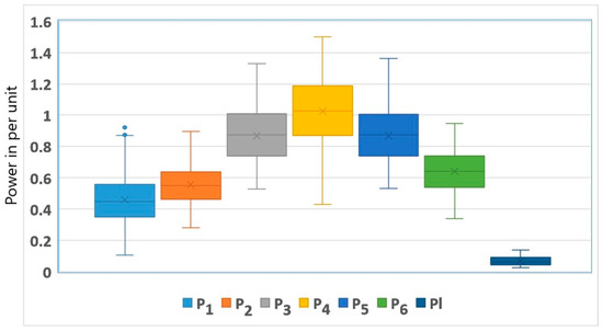
Figure 1.
Box plot of the dataset used for the training and testing of random forest model.
Table 1 provides a sample of the dataset with seven attributes and rows. The maximum and minimum value of the transmission loss were p.u. and p.u., respectively.

Table 1.
Sample data for training the random forest model to predict the transmission loss.
5.2. Random Forest Machine Learning Model
A random forest is a supervised machine-learning model that consists of multiple decision trees [43]. Decision tree models are known to overfit, and hence to reduce the problem of overfitting, an ensemble of decision trees called random forests is used for prediction. The output of the random forest is the mean value of the output from all the individual learners or the decision trees. Random forests employs a technique called feature bagging, where only a subset of features is used during the growth of the individual decision trees. A random forest regression model is an ensemble learning technique that makes accurate predictions compared to any machine learning model [44].
The random forest model in MATLAB has been developed using the regression learner app, which enables automated training to choose the best ensemble model. The train–test split ratio was 70:30. In the dataset, a random split of 8600 data was used for training the random forest model and the remaining 3400 data were used for testing the model. An optimizable ensemble preset model in the application was used for model development, including the option for hyperparameter tuning using Bayesian optimization and five-fold cross-validation. Even though the K-fold cross-validation scheme needs multiple fits to access the predictive accuracy, it is preferred as it uses the available data efficiently and works very well for a small dataset. Furthermore, Bayesian optimization techniques were preferred over the most commonly used grid research or random search method, as these techniques independently explore the whole range of possible parameter values without considering the previous outcomes. Furthermore, as the number of hyperparameters increases, the search time for the grid search and random search methods also increases exponentially. To overcome these drawbacks, Bayesian optimization techniques, which focus on promising areas of hyperparameter space, are employed, and this technique, based on the information encountered so far, predicts the next set of hyperparameters [45]. The list of hyperparameters and their values are shown in Table 2. The value of the hyperparameters during tuning using the Bayesian algorithm is shown in Table 3. The maximum objective function evaluations were set to 30. The best hyperparameter, which reduced the objective function value, is shown in bold. The mean squared error (MSE) obtained during tuning of hyperparameters is shown in Figure 2. The total time taken for hyperparameter tuning was 430 s.

Table 2.
List of hyperparameters and their value employed during tuning using Bayesian optimization.

Table 3.
Values of the hyperparameters during each iteration of tuning.
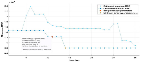
Figure 2.
Mean squared error curve during tuning of hyperparameters.
The best model had a root mean square of 0.0011571, an R-squared value almost equal to one, and a mean squared error value of 1.22 × 10⁻⁶, which was very close to the ANN model [29] whose mean squared error value was 1 × 10⁻⁸. These statistical measures indicate that the random forest model could accurately predict transmission loss. The accuracy of the prediction of the trained model is indicated by the response plot shown in Figure 2.
A 45-degree line in Figure 3 indicates that the random forest ensemble was able to accurately predict the transmission loss. Furthermore, the variable plots shown in Figure 4, Figure 5, Figure 6, Figure 7, Figure 8 and Figure 9 indicate that the error was significantly less between actual and predicted values.
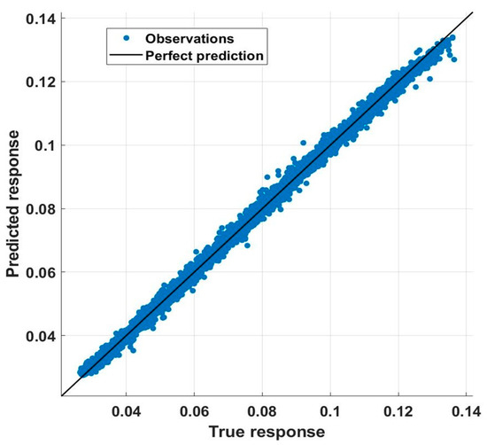
Figure 3.
Response plot between the actual and predicted transmission loss.
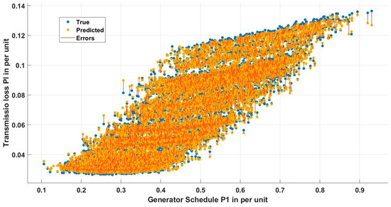
Figure 4.
Variable plot between the schedule P1 and predicted transmission loss.
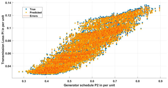
Figure 5.
Variable plot between the schedule P2 and predicted transmission loss.
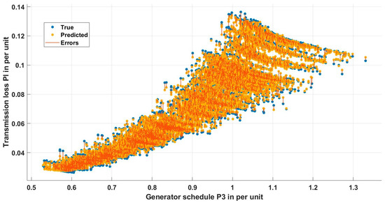
Figure 6.
Variable plot between the schedule P3 and predicted transmission loss.
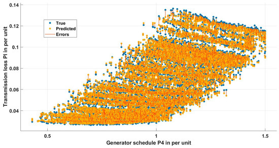
Figure 7.
Variable plot between the schedule P4 and predicted transmission loss.
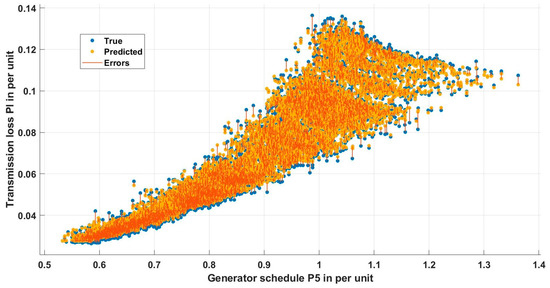
Figure 8.
Variable plot between the schedule P5 and predicted transmission loss.
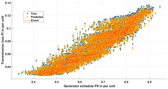
Figure 9.
Variable plot between the schedule P6 and predicted transmission loss.
The random forest regression model, meticulously developed and fine-tuned using MATLAB’s regression learner app, emerged as a powerful tool for predicting transmission loss. Its ensemble nature, composed of multiple decision trees, effectively mitigates the risk of overfitting associated with individual tree models. Through the use of feature bagging and Bayesian optimization with five-fold cross-validation, the model demonstrated robustness and efficiency in training. The careful selection of hyperparameters detailed in Table 3 resulted in a mean squared error of 1.22 × 10⁻⁶, showcasing the model’s exceptional accuracy. Key statistical measures, including a root mean square of 0.0011571 and an R-squared value approaching unity, affirmed the precision and reliability of the model. Visual representations, such as the response plot in Figure 2 and variable plots in Figure 4, Figure 5, Figure 6, Figure 7, Figure 8 and Figure 9, further underscore the proficiency of the random forest ensemble in accurately predicting the transmission loss. The thorough evaluation from hyperparameter tuning to statistical metrics and visual representations collectively supported the assertion that the meticulously crafted and optimized random forest regression model stands as a robust and accurate tool for predicting the transmission loss, contributing both to predictive modeling advancements and practical insights into transmission loss dynamics in the studied dataset.
6. Proposed Algorithm for DEED Incorporating Random Forest Based Loss Prediction
The lossless dispatch DEED problem is easier to solve and converges rapidly compared to the DEED problem incorporated with real power transmission losses. Hence, the MOSPO algorithm was developed only to solve a lossless dispatch to satisfy the demand at any moment t of the dispatch period until the algorithm reaches a quarter of the maximum iteration value. When the iteration counter is equal to a quarter of the maximum iteration value, the MOSPO algorithm using the fuzzy decision approach [18,19,20,46] selects the best compromise solution from the list of available compromise solutions. The schedule of the generators available in the best compromise solution is used as an input to the trained random forest model to predict the transmission loss . Until the iteration counter reaches the maximum value, the MOSPO algorithm will only run a lossless dispatch, with the demand increased to demand plus losses . Once the MOSPO algorithm is completed, the best compromise solution is selected based on the fuzzy decision-making approach. The main advantage of the proposed algorithm lies in the fact that load flow equations are not solved to find the transmission loss, nor are B-loss coefficients used, but only an offline-trained random forest model predicts the transmission loss once during the algorithm. The algorithmic steps of the proposed algorithm using MOSPO are provided in Figure 10 with the novelty indicated in orange color. The main advantage of the MOSPO algorithm compared to widely used algorithms, such as MOPSO and hybrid NSGAII-MOPSO algorithms, is that it has the fewest parameters compared to any other algorithm. When the number of parameters increases, finding the ideal combination becomes cumbersome. MOSPO has only 6 parameters, MOPSO has 9, and the hybrid NSGAII-MOPSO algorithm has 14 parameters.
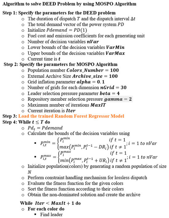
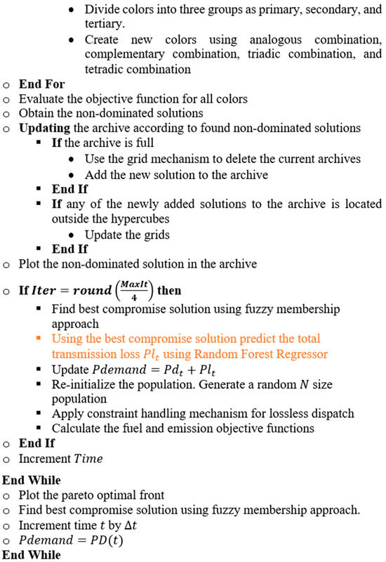
Figure 10.
Proposed algorithm to solve the dynamic economic emission dispatch.
The proposed algorithm for dynamic economic emission dispatch (DEED) embodies a strategic approach, leveraging the multi-objective stochastic paint optimizer (MOSPO) framework and integrating a random forest-based loss prediction to efficiently address real power transmission complexities. Initially employing lossless dispatch for rapid convergence, MOSPO dynamically transitions to consider transmission losses using a trained random forest model. The algorithm’s distinctive feature lies in its ability to bypass load flow equations and B-loss coefficients, relying solely on the predictive capabilities of the random forest model. This streamlined approach not only enhances computational efficiency but also minimizes the need for iterative calculations. Illustrated in Figure 10, the algorithmic steps showcase the novelty in orange, emphasizing the unique contributions. Critically, MOSPO’s simplicity shines through with a minimal parameter set—only six parameters—setting it apart from more complex algorithms such as MOPSO and hybrid NSGAII-MOPSO. This simplicity expedites the search for optimal parameter combinations and positions MOSPO as an efficient and effective tool for solving the DEED problem with real-world power system constraints.
7. Case Studies
In this section, the efficacy of the MOSPO algorithm in solving the DEED problem with B-loss coefficients and using the proposed random forest regressor model is carried out. First, the effectiveness of the MOSPO and its competitive performance is established using 5 and 10 thermal units with valve point effects and a B-loss coefficient. Furthermore, MOSPO is tested with an IEEE 30 bus test system consisting of six thermal units using the proposed random forest-based loss prediction algorithm. The chosen case studies, involving 5 and 10 thermal units with valve point effects, and the IEEE 30 bus test system with 6 thermal units, are widely utilized in the literature. This selection allows for an easy comparison of results with existing techniques, ensuring a comprehensive evaluation of the MOSPO algorithm’s performance in addressing the DEED problem with B-loss coefficients.
Unless specified in the case study, the parameters of the MOSPO algorithm were set as shown in Figure 10 and this was based on the recommendation in [41] demonstrating its effectiveness in complex benchmark functions and also on the complexity of the test system adopted. To ensure fairness, the parameters of the competing algorithms were obtained from their respective research work and are summarized in Table 4 along with the MOSPO algorithm. As seen from Table 4, the population of MOSPO was very reasonable and the iteration count was the least when compared to any other algorithm.

Table 4.
Parameters of the competing algorithms along with MOSPO.
7.1. Case 1—Five-Unit Test System
The five-unit test system considered in [4] was employed in this case study. A dynamic economic dispatch was considered for a day with a dispatch interval of 1 h. The transmission loss was modeled using the B-loss coefficients that are available in [4]. The up-ramp limits for generators 1 to 5 were 30 MW/h, 30 MW/h, 40 MW/h, 50 MW/h, and 50 MW/h respectively. The down-ramp limits for generators 1 to 5 were 30 MW/h, 30 MW/h, 40 MW/h, 50 MW/h, and 50 MW/h respectively. The proposed algorithm was run 20 times. The time elapsed for each run, the total emission, and the total fuel cost obtained for each run are summarized in Table 5. As seen from Table 5, the average time required by the proposed algorithm to find the PO solutions for a 24 h dispatch with 1 h intervals was s. This time includes the convergence time of the algorithm along with time for plotting the PO solutions for each hour, and the printing of results.

Table 5.
Summary of the results obtained for five-unit test system.
The PO solutions obtained using the MOPSO algorithm for the first twenty runs are shown as red dots and the non-Pareto solutions are shown as black dots in Figure 11. The compromise solution obtained using the fuzzy membership method is shown as a blue dot in Figure 11. The generator schedules of the compromise solution are tabulated in Table 6 along with the demand, the total generation, and the transmission loss for each hour. The emission levels and fuel cost obtained for each hour are also tabulated. From the schedules obtained we can observe that the minimum and maximum generator limits for all generators were satisfied, along with the ramp limit constraints for the entire dispatch.
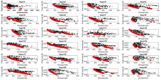
Figure 11.
Non-Pareto-optimal solutions (black dot), PO Solutions (red dot), and compromise solution (blue dot) for each hour of the dispatch period for the five-unit system.

Table 6.
The schedules of the generators obtained for the dynamic dispatch for the five-unit system.
From Table 6, we can infer that the minimum demand of 410 MW occurred at 1 AM and the maximum demand of 740 MW occurred at 12 noon. Even though the demand pattern changed throughout the day, only one B-loss coefficient was used during the dispatch period. As the B-loss coefficients are determined for a specific load level, use of these coefficients will only result in an approximate loss calculation at all other load levels. The main idea of this research is to overcome this drawback and to replace this approximate B-loss formula with a transmission loss prediction. In this case study, the MOSPO algorithm was used along with approximate B-loss formula only to ensure the fairness of the comparison with the existing algorithm
Figure 12 compares the total emission and total fuel cost of the dispatch obtained using the MOSPO algorithm with several existing algorithms. In Figure 12, the red color and bold indicate that the MOSPO algorithm could outperform the existing algorithms in that specific objective. Out of the 14 algorithms compared, MOSPO could outperform five algorithms in both objectives, six algorithms in at least one objective, and it could not outperform three algorithms in any objective.
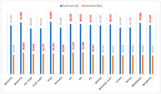
Figure 12.
Comparison of the fuel costs and emissions obtained using the MOSPO algorithm with the MOPPO [21], DE-SQP [12], PSO-SQP [12], PSO [3], NPAHS [7], EP [4], SA [5], PS [5], MODE [20], MOHDE-SAT [20], EFDE [9], NEHS [8], MONNDE [22] and MOMVO [29] for the five-unit systems. The red color and bold indicate that the MOSPO algorithm could outperform the existing algorithms in that specific objective.
7.2. Case 2—Ten-Unit Test System
A widely used 10-unit test system was employed in this case study. The fuel cost data for the ten thermal generators, the load profile, and a single B-loss coefficient for the entire time horizon are available in [15], and the maximum iteration count for the MOSPSO algorithm was set to 100. The stacked bar plot of the generator schedules is shown in Figure 13. The schedule of the ten generators for each hour obtained using the MOSPO algorithm is tabulated in Table 7.
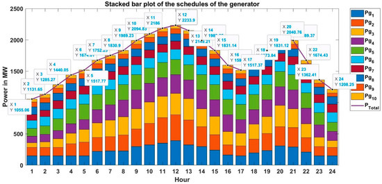
Figure 13.
Stacked bar plot of the schedules for the generator obtained using MOPSO.

Table 7.
The schedules of the generators obtained for the DEED for the ten-unit system.
Figure 14 compares the results obtained using the MOSPO algorithm with several existing algorithms. In Figure 14, the red color and bold indicate that the MOSPO algorithm could outperform the existing algorithms in that specific objective. The MOSPO algorithm outperformed the following nine state-of-the-art algorithms: MOPPO [21], SPSO [6], NSGA-II [15], IBFA [47], RCGA [15], MAMODE [19], CRO [11], HCRO [11], and MODE [20] in both objectives. The MOSPO algorithm can outperform the following existing algorithms MOMVO [29], PSOAWL [6], MOHDE-SAT [20], DE-SQP [12], PSO-SQP [12], EFDE [9], NEHS [8], and MONNDE [22] in at least one objective.
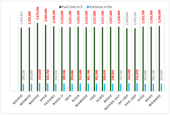
Figure 14.
Comparison of the fuel costs and emissions obtained using the MOSPO algorithm with the existing algorithms for the ten-unit systems. The red color and bold indicate that the MOSPO algorithm could outperform the existing algorithms in that specific objective.
7.3. Case 3—IEEE 30 Bus Test System
An IEEE 30 bus power system with thermal generators was used in this case study. The fuel cost and emission data are available in [17,18]. The ramp-up and ramp-down limits were set at p.u. The offline-trained random forest regression model presented in Section 5 was used to predict the transmission loss during each hour of the dispatch period. A base value of MW was used for the per-unit calculations. All existing algorithms except [29] use only one B-loss coefficient for the demand, which varies widely from a based load of p.u. to the peak load of p.u. Using one B-loss coefficient for the entire dispatch period will not provide an accurate transmission loss, but the trained random forest model will be able to predict the loss accurately.
The proposed algorithm integrated with loss prediction was run 20 times and the results obtained are summarized in Table 8. The load demand shown in column 2 of Table 9 was considered to obtain a comprehensive analysis. The average time the algorithm took to converge was s. This time included the convergence time of the algorithm along with loss prediction, time for plotting the PO solutions for each hour, and the printing of results. The results indicate the robustness and consistency of the proposed algorithm in obtaining reliable and feasible results. Comparing the maximum, minimum, and average values of the time, emission, and fuel cost indicated the high level of convergence obtained using the proposed algorithm in obtaining the PO solutions.

Table 8.
Summary of the results obtained for IEEE 30 bus test system.

Table 9.
The schedules of the generators obtained for the DEED using the MOSPO algorithm for the IEEE 30 bus test system.
The results obtained for the 21st run of the proposed algorithm are shown in Table 9. The maximum iteration count for the MOSPO algorithm was set as 40. Until the iteration count reached 10 during every hour of the dispatch period, a lossless dispatch was carried out, and when the count reached 10 the compromise solution obtained using the MOSPO algorithm was used by the random forest model to predict the transmission loss. Using this transmission loss, the total demand at that hour is increased to . Starting from the iteration count 11 to 40, the MOSPO algorithm solves a lossless dispatch to satisfy the demand . The fuzzy membership function is used at the end of the iteration to find the best compromise solution. For example, let us take hour 5. Until the iteration count reaches ten, the MOSPO algorithm solves a lossless dispatch to satisfy the demand p.u. When the count reaches 10, the random forest algorithm predicts the loss for the compromise solution as p.u. From iteration count 11 to 40, the MOSPO algorithm solves a lossless dispatch to satisfy a demand of p.u. A fuzzy membership approach is applied to find the compromise solution at the end of the iteration, and the schedules of the generators are shown in Table 8. The transmission loss obtained during each hour of the dispatch period was cross-verified using power flow analysis, and the loss obtained using power flow analysis exactly matches the loss predicted by the random forest algorithm. The PO solutions (red dot) and compromise solution (blue dot) for each hour of the dispatch period for the IEEE 30 bus system are shown in Figure 15.
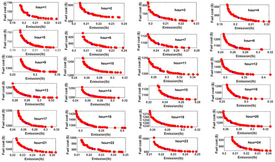
Figure 15.
PO Solutions (red dot) and compromise solution (blue dot) for each hour of the dispatch period for the IEEE 30 bus system.
The results obtained using the MOSPO algorithm were compared with the GSOMP algorithm in [17] and the MOMVO algorithm in [29]. The fuel cost and emission levels obtained for the best compromise solution using the GSOMP algorithm and MOMVO algorithm were USD and and USD respectively. The emission level obtained using the MOSPO algorithm was which was almost the same as the other existing algorithms. The savings in the fuel cost obtained using the MOSPO algorithm are compared in Table 10. Table 10 shows the yearly savings obtained using the MOSPO algorithm compared to the GSOMP algorithm and MOMVO algorithm, and these were USD 37,339.5 and USD 3423.7, respectively. The time taken by the GSOMP algorithm was 1262.93 s, and this algorithm could outperform the NSGAII and MOSPO algorithms, as shown in [17]. The average time taken by the MOSPO algorithm was 1038.47 s, and it was much faster when compared to the time taken by the GSOMP algorithm.

Table 10.
Fuel cost savings obtained using the MOSPO algorithm for the IEEE 30 bus system.
8. Conclusions and Future Research Direction
In conclusion, this study presents a pioneering approach to tackling the highly strenuous and challenging bi-objective dynamic economic emission dispatch (DEED) model. The integration of a potent multi-objective stochastic paint optimizer (MOSPO) algorithm proved effective in addressing the complexities of the DEED problem, showcasing its superiority in solving both the fuel cost minimization and the pollutant emission reduction objectives. A key innovation lies in the incorporation of a random forest regression model, trained to predict the transmission loss specifically for the IEEE 30 bus system. This novel integration of machine learning into the DEED model overcomes the challenges associated with solving complex B-loss coefficients or conducting load flow analysis during each iteration. The elimination of these computational burdens significantly enhances the efficiency of the MOSPO algorithm.
This study initially establishes the effectiveness and superiority of the MOSPO algorithm by comparing its performance on five-unit and ten-unit systems. The results demonstrated that MOSPO outperforms most algorithms in at least one objective, affirming its robustness in solving the DEED problem. Notably, the MOSPO algorithm exhibited a faster convergence compared to the existing algorithms, further highlighting its efficiency. Subsequently, the random forest model, incorporated into MOSPO, was applied to solve the DEED for the IEEE 30 bus system. The achieved yearly fuel cost savings of USD 37,339.5 (0.396%) and USD 3423.7 (0.036%) when compared to existing GSOMP and MOMVO algorithms, respectively, underscoring the economic benefits of the MOSPO algorithm. Beyond cost savings, the algorithm’s faster convergence adds another dimension to its practical applicability in real-time power system operations.
Looking ahead, future research endeavors could delve into expanding the algorithm’s applicability to even larger and more complex power systems. The integration of additional machine learning techniques or optimization algorithms could further enhance the algorithm’s performance and broaden its scope. Improving the predictive capabilities of the random forest model by incorporating real-time data and accommodating dynamic changes in the power system remains an avenue worth exploring. Additionally, extending the application of the proposed approach to address other optimization challenges within power systems, such as unit commitment or economic dispatch with renewable energy sources, could contribute to a more comprehensive understanding of its capabilities.
In summary, future research should aim at advancing the algorithm’s adaptability, refining its predictive capabilities, and exploring new domains within power system optimization. These efforts would further solidify the MOSPO algorithm’s position as a robust and efficient solution for dynamic economic emission dispatch problems, fostering sustainability and efficiency in power system operations.
Author Contributions
Conceptualization, A.S. and N.S.A.; methodology, A.S.; software, A.S.; validation, N.S.A. formal analysis, A.S., resources, N.S.A.; writing—original draft preparation, A.S.; writing—review and editing, N.S.A. All authors have read and agreed to the published version of the manuscript.
Funding
This research received no external funding.
Data Availability Statement
A link to download the data has been provided: https://doi.org/10.24433/CO.5812681.v1 accessed on 7 January 2024.
Acknowledgments
The authors would like to thank the facilities provided by the authorities of the Royal Commission of Jubail and Yanbu, and the management of Jubail Industrial College to carry out this research.
Conflicts of Interest
The authors declare no conflicts of interest.
References
- Liu, C.; Shahidehpour, M.; Li, Z.; Fotuhi-Firuzabad, M. Component and Mode Models for the Short-Term Scheduling of Combined-Cycle Units. IEEE Trans. Power Syst. 2009, 24, 976–990. [Google Scholar] [CrossRef]
- Chiang, C.L. Improved Genetic Algorithm for Power Economic Dispatch of Units with Valve-Point Effects and Multiple Fuels. IEEE Trans. Power Syst. 2005, 20, 1690–1699. [Google Scholar] [CrossRef]
- Basu, M. Particle Swarm Optimization Based Goal-Attainment Method for Dynamic Economic Emission Dispatch. Electr. Power Compon. Syst. 2006, 34, 1015–1025. [Google Scholar] [CrossRef]
- Basu, M. Dynamic Economic Emission Dispatch Using Evolutionary Programming and Fuzzy Satisfying Method. Int. J. Emerg. Electr. Power Syst. 2007, 8. [Google Scholar] [CrossRef]
- Alsumait, J.S.; Qasem, M.; Sykulski, J.K.; Al-Othman, A.K. An Improved Pattern Search Based Algorithm to Solve the Dynamic Economic Dispatch Problem with Valve-Point Effect. Energy Convers. Manag. 2010, 51, 2062–2067. [Google Scholar] [CrossRef]
- Mason, K.; Duggan, J.; Howley, E. Multi-Objective Dynamic Economic Emission Dispatch Using Particle Swarm Optimisation Variants. Neurocomputing 2017, 270, 188–197. [Google Scholar] [CrossRef]
- Niu, Q.; Zhang, H.; Li, K.; Irwin, G.W. An Efficient Harmony Search with New Pitch Adjustment for Dynamic Economic Dispatch. Energy 2014, 65, 25–43. [Google Scholar] [CrossRef]
- Li, Z.; Zou, D.; Kong, Z. A Harmony Search Variant and a Useful Constraint Handling Method for the Dynamic Economic Emission Dispatch Problems Considering Transmission Loss. Eng. Appl. Artif. Intell. 2019, 84, 18–40. [Google Scholar] [CrossRef]
- Shen, X.; Zou, D.; Duan, N.; Zhang, Q. An Efficient Fitness-Based Differential Evolution Algorithm and a Constraint Handling Technique for Dynamic Economic Emission Dispatch. Energy 2019, 186, 115801. [Google Scholar] [CrossRef]
- Parihar, S.S.; Malik, N. Fuzzy-Based Real-Coded Genetic Algorithm for Optimizing Non-Convex Environmental Economic Loss Dispatch. Facta Univ. Ser. Electron. Energetics 2022, 35, 495–512. [Google Scholar] [CrossRef]
- Roy, P.K.; Bhui, S. A Multi-Objective Hybrid Evolutionary Algorithm for Dynamic Economic Emission Load Dispatch. Int. Trans. Electr. Energy Syst. 2016, 26, 49–78. [Google Scholar] [CrossRef]
- Elaiw, A.M.; Xia, X.; Shehata, A.M. Hybrid DE-SQP and Hybrid PSO-SQP Methods for Solving Dynamic Economic Emission Dispatch Problem with Valve-Point Effects. Electr. Power Syst. Res. 2013, 103, 192–200. [Google Scholar] [CrossRef]
- Sheng, W.; Li, R.; Yan, T.; Tseng, M.L.; Lou, J.; Li, L. A Hybrid Dynamic Economics Emissions Dispatch Model: Distributed Renewable Power Systems Based on Improved COOT Optimization Algorithm. Renew. Energy 2023, 204, 493–506. [Google Scholar] [CrossRef]
- Nagarajan, K.; Rajagopalan, A.; Angalaeswari, S.; Natrayan, L.; Mammo, W.D. Combined Economic Emission Dispatch of Microgrid with the Incorporation of Renewable Energy Sources Using Improved Mayfly Optimization Algorithm. Comput. Intell. Neurosci. 2022, 2022, 6461690. [Google Scholar] [CrossRef]
- Basu, M. Dynamic Economic Emission Dispatch Using Nondominated Sorting Genetic Algorithm-II. Int. J. Electr. Power Energy Syst. 2008, 30, 140–149. [Google Scholar] [CrossRef]
- Dhanalakshmi, S.; Kannan, S.; Mahadevan, K.; Baskar, S. Application of Modified NSGA-II Algorithm to Combined Economic and Emission Dispatch Problem. Int. J. Electr. Power Energy Syst. 2011, 33, 992–1002. [Google Scholar] [CrossRef]
- Guo, C.X.; Zhan, J.P.; Wu, Q.H. Dynamic Economic Emission Dispatch Based on Group Search Optimizer with Multiple Producers. Electr. Power Syst. Res. 2012, 86, 8–16. [Google Scholar] [CrossRef]
- Wu, L.H.; Wang, Y.N.; Yuan, X.F.; Zhou, S.W. Environmental/Economic Power Dispatch Problem Using Multi-Objective Differential Evolution Algorithm. Electr. Power Syst. Res. 2010, 80, 1171–1181. [Google Scholar] [CrossRef]
- Jiang, X.; Zhou, J.; Wang, H.; Zhang, Y. Dynamic Environmental Economic Dispatch Using Multiobjective Differential Evolution Algorithm with Expanded Double Selection and Adaptive Random Restart. Int. J. Electr. Power Energy Syst. 2013, 49, 399–407. [Google Scholar] [CrossRef]
- Zhang, H.; Yue, D.; Xie, X.; Hu, S.; Weng, S. Multi-Elite Guide Hybrid Differential Evolution with Simulated Annealing Technique for Dynamic Economic Emission Dispatch. Appl. Soft Comput. J. 2015, 34, 312–323. [Google Scholar] [CrossRef]
- Shao, Z.; Si, F.; Wu, H.; Tong, X. An Agile and Intelligent Dynamic Economic Emission Dispatcher Based on Multi-Objective Proximal Policy Optimization. Appl. Soft Comput. 2021, 102, 107047. [Google Scholar] [CrossRef]
- Mason, K.; Duggan, J.; Howley, E. A Multi-Objective Neural Network Trained with Differential Evolution for Dynamic Economic Emission Dispatch. Int. J. Electr. Power Energy Syst. 2018, 100, 201–221. [Google Scholar] [CrossRef]
- Hassan, M.H.; Kamel, S.; Domínguez-García, J.L.; El-Naggar, M.F. MSSA-DEED: A Multi-Objective Salp Swarm Algorithm for Solving Dynamic Economic Emission Dispatch Problems. Sustainability 2022, 14, 9785. [Google Scholar] [CrossRef]
- Yan, L.; Zhu, Z.; Kang, X.; Qu, B.; Qiao, B.; Huan, J.; Chai, X. Multi-Objective Dynamic Economic Emission Dispatch with Electric Vehicle–Wind Power Interaction Based on a Self-Adaptive Multiple-Learning Harmony-Search Algorithm. Energies 2022, 15, 4942. [Google Scholar] [CrossRef]
- Lokeshgupta, B.; Sivasubramani, S. Dynamic Economic and Emission Dispatch with Renewable Energy Integration Under Uncertainties and Demand-Side Management. Electr. Eng. 2022, 104, 2237–2248. [Google Scholar] [CrossRef]
- Zou, D.; Gong, D.; Ouyang, H. The Dynamic Economic Emission Dispatch of the Combined Heat and Power System Integrated with a Wind Farm and a Photovoltaic Plant. Appl. Energy 2023, 351, 121890. [Google Scholar] [CrossRef]
- Arul, R.; Velusami, S.; Ravi, G. A New Algorithm for Combined Dynamic Economic Emission Dispatch with Security Constraints. Energy 2015, 79, 496–511. [Google Scholar] [CrossRef]
- Zou, D.; Li, S.; Li, Z.; Kong, X. A New Global Particle Swarm Optimization for the Economic Emission Dispatch with or without Transmission Losses. Energy Convers. Manag. 2017, 139, 45–70. [Google Scholar] [CrossRef]
- Sundaram, A. Multiobjective Multi Verse Optimization Algorithm to Solve Dynamic Economic Emission Dispatch Problem with Transmission Loss Prediction by an Artificial Neural Network. Appl. Soft Comput. 2022, 124, 109021. [Google Scholar] [CrossRef]
- Sundaram, A. Fair and Transparent Loss Allocation and Pricing in Primary Electricity Market Using the Concept of Market Center. Ph.D. Thesis, Anna University, Chennai, India, 2014. [Google Scholar] [CrossRef]
- Arunachalam, S.; Saranya, R.; Sangeetha, N. Hybrid Artificial Bee Colony Algorithm and Simulated Annealing Algorithm for Combined Economic and Emission Dispatch Including Valve Point Effect. In Swarm, Evolutionary, and Memetic Computing, Proceedings of the 4th International Conference, SEMCCO 2013, Chennai, India, 19–21 December 2013; Springer International Publishing: Cham, Switzerland, 2013; Volume 8297, pp. 354–365. [Google Scholar]
- Arunachalam, S.; AgnesBhomila, T.; Ramesh Babu, M. Hybrid Particle Swarm Optimization Algorithm and Firefly Algorithm Based Combined Economic and Emission Dispatch Including Valve Point Effect. In Swarm, Evolutionary, and Memetic Computing, Proceedings of the 5th International Conference, SEMCCO 2014, Bhubaneswar, India, 18–20 December 2014; Springer International Publishing: Cham, Switzerland, 2015; Volume 8947, pp. 647–660. [Google Scholar]
- Sundaram, A. Solution of Combined Economic Emission Dispatch Problem with Valve-Point Effect Using Hybrid NSGA II-MOPSO. In Particle Swarm Optimization with Applications; Erdogmus, P., Ed.; IntechOpen: London, UK, 2018; pp. 81–100. ISBN 978-1-78923-149-6. [Google Scholar]
- Murugan, R.; Mohan, M.R.; Asir Rajan, C.C.; Sundari, P.D.; Arunachalam, S. Hybridizing Bat Algorithm with Artificial Bee Colony for Combined Heat and Power Economic Dispatch. Appl. Soft Comput. 2018, 72, 189–217. [Google Scholar] [CrossRef]
- Sundaram, A. Multiobjective Multi-Verse Optimization Algorithm to Solve Combined Economic, Heat and Power Emission Dispatch Problems. Appl. Soft Comput. J. 2020, 91, 106195. [Google Scholar] [CrossRef]
- Sundaram, A. Combined Heat and Power Economic Emission Dispatch Using Hybrid NSGA II-MOPSO Algorithm Incorporating an Effective Constraint Handling Mechanism. IEEE Access 2020, 8, 13748–13768. [Google Scholar] [CrossRef]
- Ramachandran, M.; Mirjalili, S.; Malli Ramalingam, M.; Charles Gnanakkan, C.A.R.; Parvathysankar, D.S.; Sundaram, A. A Ranking-Based Fuzzy Adaptive Hybrid Crow Search Algorithm for Combined Heat and Power Economic Dispatch. Expert. Syst. Appl. 2022, 197, 116625. [Google Scholar] [CrossRef]
- Ramachandran, M.; Mirjalili, S.; Nazari-Heris, M.; Parvathysankar, D.S.; Sundaram, A.; Charles Gnanakkan, C.A.R. A Hybrid Grasshopper Optimization Algorithm and Harris Hawks Optimizer for Combined Heat and Power Economic Dispatch Problem. Eng. Appl. Artif. Intell. 2022, 111, 104753. [Google Scholar] [CrossRef]
- Wolpert, D.H.; Macready, W.G. No Free Lunch Theorems for Optimization. IEEE Trans. Evol. Comput. 1997, 1, 67. [Google Scholar] [CrossRef]
- Kaveh, A.; Talatahari, S.; Khodadadi, N. Stochastic Paint Optimizer: Theory and Application in Civil Engineering. Eng. Comput. 2020, 38, 1921–1952. [Google Scholar] [CrossRef]
- Khodadadi, N.; Abualigah, L.; Mirjalili, S. Multi-Objective Stochastic Paint Optimizer (MOSPO). Neural Comput. Appl. 2022, 134, 18035–18058. [Google Scholar] [CrossRef]
- Coello Coello, C.A.; Lechuga, M.S. MOPSO: A Proposal for Multiple Objective Particle Swarm Optimization. In Proceedings of the 2002 Congress on Evolutionary Computation. CEC’02 (Cat. No.02TH8600), Honolulu, HI, USA, 12–17 May 2002; IEEE: Piscataway, NJ, USA, 2002; Volume 2, pp. 1051–1056. [Google Scholar]
- Liu, Y.; Wang, Y.; Zhang, J. New Machine Learning Algorithm: Random Forest. In Information Computing and Applications, Proceedings of the Third International Conference, ICICA 2012, Chengde, China, 14–16 September 2012; Springer: Berlin/Heidelberg, Germany, 2012; Volume 7473, pp. 246–252. [Google Scholar] [CrossRef]
- Segal, M.R. Machine Learning Benchmarks and Random Forest Regression; University of California: San Francisco, CA, USA, 2004. [Google Scholar]
- Wu, J.; Chen, X.Y.; Zhang, H.; Xiong, L.D.; Lei, H.; Deng, S.H. Hyperparameter Optimization for Machine Learning Models Based on Bayesian Optimization. J. Electron. Sci. Technol. 2019, 17, 26–40. [Google Scholar] [CrossRef]
- Qiao, B.; Liu, J.; Hao, X. A Multi-Objective Differential Evolution Algorithm and a Constraint Handling Mechanism Based on Variables Proportion for Dynamic Economic Emission Dispatch Problems. Appl. Soft Comput. 2021, 108, 107419. [Google Scholar] [CrossRef]
- Pandit, N.; Tripathi, A.; Tapaswi, S.; Pandit, M. An Improved Bacterial Foraging Algorithm for Combined Static/Dynamic Environmental Economic Dispatch. Appl. Soft Comput. J. 2012, 12, 3500–3513. [Google Scholar] [CrossRef]
Disclaimer/Publisher’s Note: The statements, opinions and data contained in all publications are solely those of the individual author(s) and contributor(s) and not of MDPI and/or the editor(s). MDPI and/or the editor(s) disclaim responsibility for any injury to people or property resulting from any ideas, methods, instructions or products referred to in the content. |
© 2024 by the authors. Licensee MDPI, Basel, Switzerland. This article is an open access article distributed under the terms and conditions of the Creative Commons Attribution (CC BY) license (https://creativecommons.org/licenses/by/4.0/).