
The Nexus between Wholesale Electricity Prices and the Share of Electricity Production from Renewables: An Analysis with and without the Impact of Time of Distress


Abstract
1. Introduction
- (1)
- To review the wholesale electricity market in detail and the key factors affecting WHEP, primarily focusing on the role of RES in it;
- (2)
- To assess whether the selected factors have statistically significant relationships with WHEP, and if so, estimate the extent of the contributions in the different circumstances.
2. Literature Review
2.1. The Wholesale Electricity Market and the Key Factors Affecting the Prices
2.2. State of the Art
3. Data and Methods
3.1. Data Description
3.2. Methodological Framework
4. Results
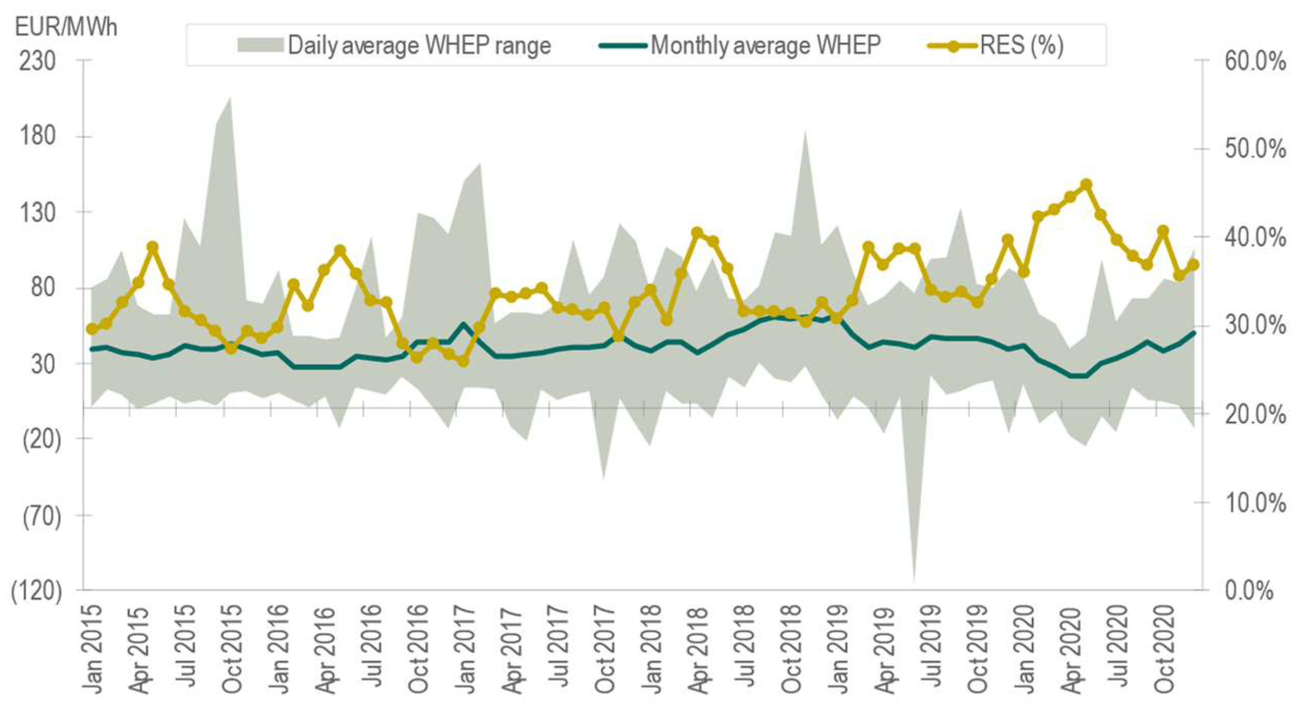
4.1. Analyzing the Pre-Crisis Period (January 2015–December 2020)
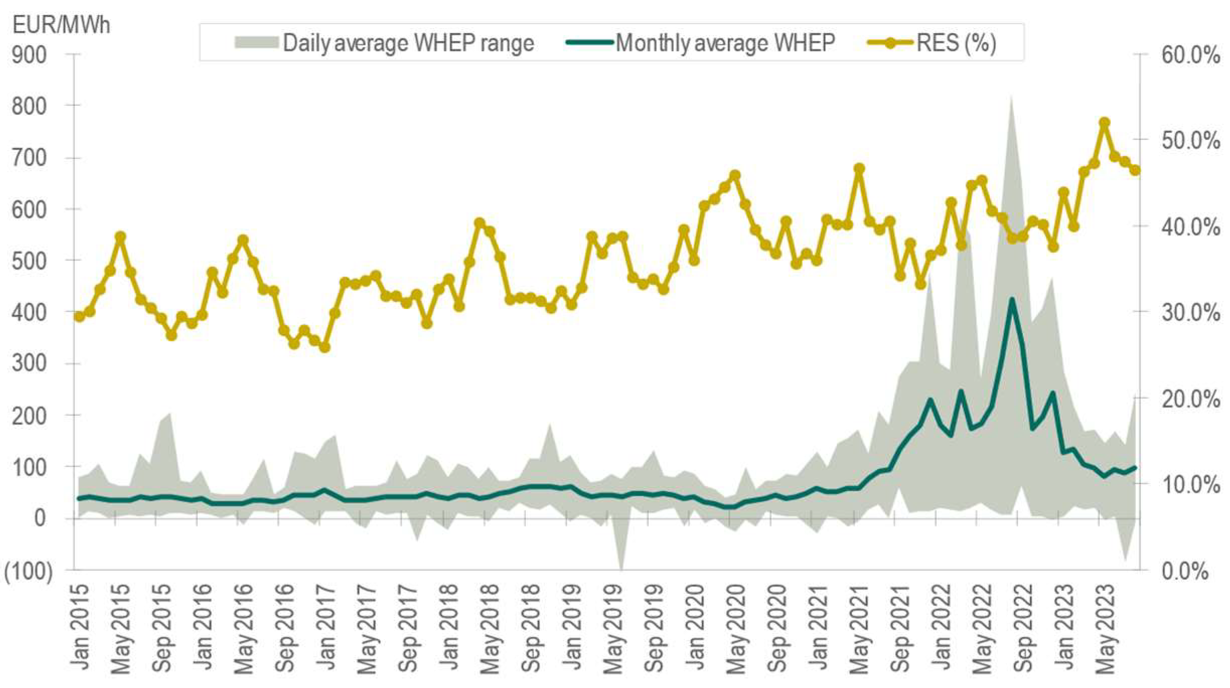
4.2. Assessing the Co-Crisis Period (January 2015–August 2023)
5. Discussion
6. Conclusions
Author Contributions
Funding
Data Availability Statement
Conflicts of Interest
Appendix A

| Variable | Transformation | ADF Test | PP Test | KPSS Test | Conclusion |
|---|---|---|---|---|---|
| WHEP | Original | 0.22 | 0.26 | 0.02 | The series is non-stationary |
| Natural logarithm | 0.27 | 0.23 | 0.03 | The series is non-stationary | |
| Log-differentiated | <0.01 | <0.01 | >0.10 | The series is stationary | |
| NEG | Original | <0.01 | <0.01 | >0.10 | The series is stationary |
| Natural logarithm | <0.01 | <0.01 | >0.10 | The series is stationary | |
| Log-differentiated | <0.01 | <0.01 | >0.10 | The series is stationary | |
| RES | Original | <0.01 | 0.02 | >0.10 | The series is stationary |
| Natural logarithm | <0.01 | <0.01 | >0.10 | The series is stationary | |
| Log-differentiated | <0.01 | <0.01 | >0.10 | The series is stationary | |
| TTF | Original | 0.27 | 0.56 | 0.02 | The series is non-stationary |
| Natural logarithm | 0.29 | 0.47 | 0.02 | The series is non-stationary | |
| Log-differentiated | <0.01 | <0.01 | >0.10 | The series is stationary | |
| BRENT | Original | 0.61 | 0.59 | <0.01 | The series is non-stationary |
| Natural logarithm | 0.57 | 0.50 | <0.01 | The series is non-stationary | |
| Log-differentiated | <0.01 | <0.01 | >0.10 | The series is stationary | |
| NEWC | Original | 0.71 | 0.84 | <0.01 | The series is non-stationary |
| Natural logarithm | 0.61 | 0.83 | <0.01 | The series is non-stationary | |
| Log-differentiated | 0.42 | <0.01 | >0.10 | The series is trend stationary | |
| EUA | Original | 0.63 | 0.80 | <0.01 | The series is non-stationary |
| Natural logarithm | 0.59 | 0.85 | <0.01 | The series is non-stationary | |
| Log-differentiated | 0.29 | <0.01 | >0.10 | The series is trend stationary |
| WHEP | NEG | RES | TTF | BRENT | NEWC | EUA | |
|---|---|---|---|---|---|---|---|
| Mean | 40.97 | 230.08 | 0.34 | 16.32 | 55.41 | 76.37 | 14.70 |
| Minimum | 21.55 | 194.31 | 0.26 | 4.94 | 26.63 | 49.40 | 4.31 |
| Maximum | 61.44 | 273.26 | 0.46 | 27.95 | 80.63 | 117.78 | 31.39 |
| Range | 39.89 | 78.95 | 0.20 | 23.01 | 54.00 | 68.37 | 27.08 |
| Std. dev. | 8.73 | 19.18 | 0.04 | 4.93 | 12.13 | 20.42 | 9.22 |
| Coeff. var. | 0.21 | 0.08 | 0.13 | 0.30 | 0.22 | 0.27 | 0.63 |
| Skewness | 0.36 | 0.41 | 0.54 | −0.22 | −0.08 | 0.41 | 0.34 |
| Kurtosis | 0.39 | −0.70 | −0.09 | −0.04 | −0.43 | −1.10 | −1.65 |
| Observations | 72 | 72 | 72 | 72 | 72 | 72 | 72 |
| WHEP | NEG | RES | TTF | BRENT | NEWC | EUA | |
|---|---|---|---|---|---|---|---|
| Mean | 75.56 | 228.58 | 0.36 | 35.15 | 64.15 | 124.40 | 32.51 |
| Minimum | 21.55 | 194.31 | 0.26 | 4.94 | 26.63 | 49.40 | 4.31 |
| Maximum | 425.20 | 273.26 | 0.52 | 235.96 | 117.50 | 439.43 | 92.61 |
| Range | 403.65 | 78.95 | 0.26 | 231.02 | 90.87 | 390.02 | 88.29 |
| Std. dev. | 71.92 | 19.09 | 0.06 | 41.84 | 18.55 | 98.51 | 29.51 |
| Coeff. var. | 0.95 | 0.08 | 0.15 | 1.19 | 0.29 | 0.79 | 0.91 |
| Skewness | 2.51 | 0.47 | 0.41 | 2.66 | 0.60 | 1.96 | 0.91 |
| Kurtosis | 6.92 | −0.71 | −0.35 | 7.55 | 0.32 | 2.84 | −0.67 |
| Observations | 104 | 104 | 104 | 104 | 104 | 104 | 104 |
| February 2015–December 2020 | ∆ * | February 2015–August 2023 | Expected Relationship ** | ||
|---|---|---|---|---|---|
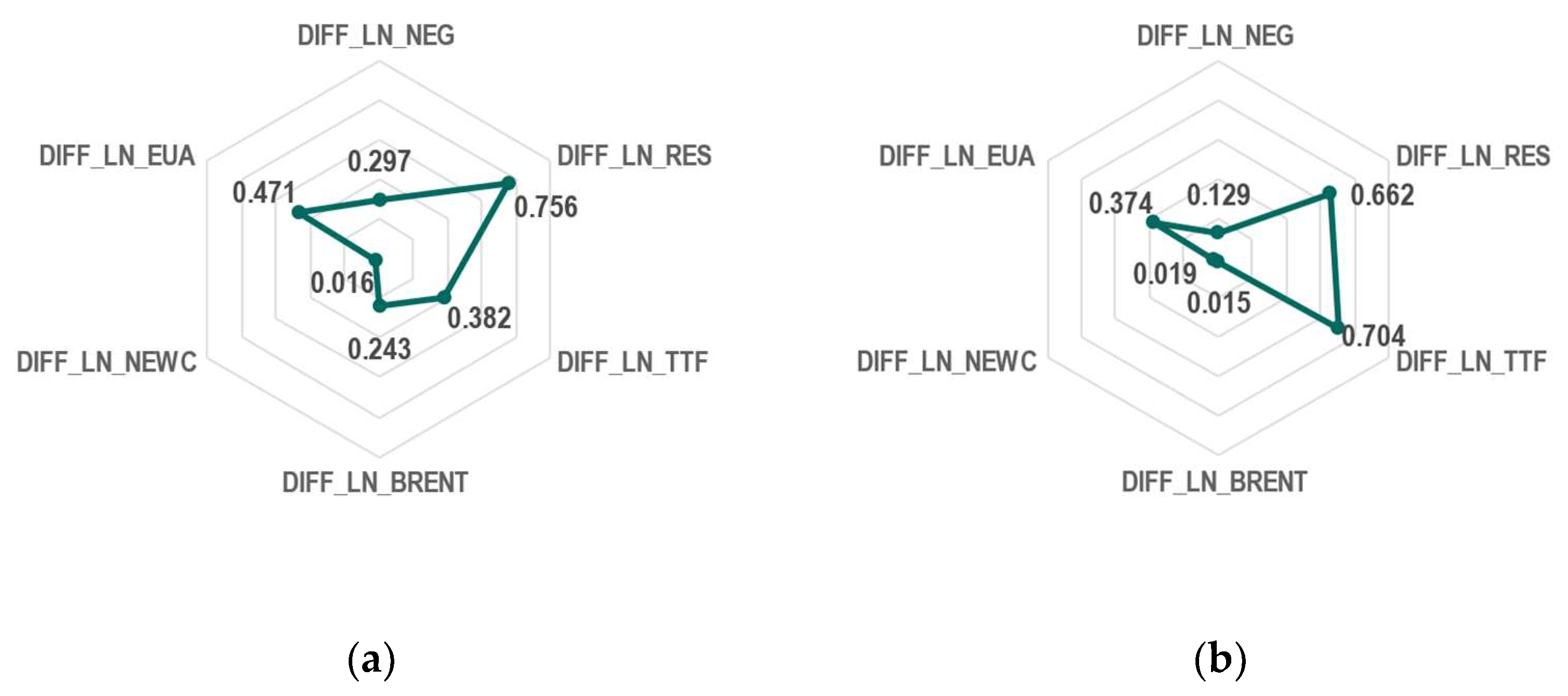
| DIFF_LN_NEG | Correlation | 0.297 | ↓ | 0.129 | +1 |
| Sign. (2-tailed) | 0.015 | 0.206 | |||
| DIFF_LN_RES | Correlation | −0.756 | ↓ | −0.662 | −3 |
| Sign. (2-tailed) | 0.000 | 0.000 | |||
| DIFF_LN_TTF | Correlation | 0.382 | ↑ | 0.704 | +3 |
| Sign. (2-tailed) | 0.002 | 0.000 | |||
| DIFF_LN_BRENT | Correlation | 0.243 | ↓ | 0.015 | +1 |
| Sign. (2-tailed) | 0.049 | 0.883 | |||
| DIFF_LN_NEWC | Correlation | −0.016 | ↑ | 0.019 | +2 |
| Sign. (2-tailed) | 0.897 | 0.851 | |||
| DIFF_LN_EUA | Correlation | 0.471 | ↓ | 0.374 | +2 |
| Sign. (2-tailed) | 0.000 | 0.000 |
| Coefficients | February 2015–December 2020 | February 2015–August 2023 | ||||||
|---|---|---|---|---|---|---|---|---|
| MLR | CO adj. MLR | Lower Bound * | Upper Bound * | MLR | CO adj. MLR | Lower Bound * | Upper Bound * | |
| DIFF_LN_NEG | 0.308 | 0.267 | 0.018 | 0.517 | ||||
| DIFF_LN_RES | −0.935 | −0.956 | −1.157 | −0.754 | −0.972 | −0.973 | −1.188 | −0.757 |
| DIFF_LN_TTF | 0.216 | 0.195 | 0.079 | 0.312 | 0.560 | 0.549 | 0.451 | 0.647 |
| DIFF_LN_BRENT | 0.154 | 0.180 | 0.039 | 0.321 | ||||
| DIFF_LN_NEWC | ||||||||
| DIFF_LN_EUA | 0.368 | 0.343 | 0.185 | 0.501 | 0.368 | 0.364 | 0.186 | 0.542 |
| R | 0.872 | 0.889 | 0.880 | 0.882 | ||||
| R square | 0.760 | 0.790 | 0.774 | 0.778 | ||||
| Adjusted R square | 0.742 | 0.770 | 0.767 | 0.769 | ||||
| Std. error of estimate | 0.064 | 0.064 | 0.086 | 0.086 | ||||
| F-stat | 41.234 | 48.000 | 112.971 | 113.236 | ||||
| p-value (F-stat) | 0.000 | 0.000 | 0.000 | 0.000 | ||||
| Durbin–Watson stat | 2.377 | 2.101 | 2.158 | 2.034 | ||||
| VIFmax | 1.199 | 1.130 | ||||||
| N | 71 | 71 | 103 | 103 | ||||
References
- Szczepanski, M. A Decade on from the Crisis: Main Responses and Remaining Challenges; European Parliamentary Research Service: Brussels, Belgium, 2019. [Google Scholar]
- International Energy Agency. Energy Policies of IEA Countries: The European Union 2014 Review; International Energy Agency: Paris, France, 2014. [Google Scholar]
- Varro, L.; Beyer, S.; Journeay-Kaler, P.; Gaffney, K. Green Stimulus after the 2008 Crisis; International Energy Agency: Paris, France, 2020. [Google Scholar]
- Houtman, A.; Reins, L. Energy Transition in the EU: Targets, Market Regulation and Law. In The Palgrave Handbook of Zero Carbon Energy Systems and Energy Transitions: Palgrave Studies in Energy Transitions; Palgrave Macmillan: Cham, Switzerland, 2022; pp. 1–26. ISBN 978-3-030-74380-2. [Google Scholar]
- European Commission. Energy 2020 A Strategy for Competitive, Sustainable and Secure Energy; European Commission: Brussels, Belgium, 2010.
- Eurostat. Statistical Database. Gross Production of Electricity and Derived Heat from Non-Combustible Fuels by Type of Plant and Operator. Available online: https://ec.europa.eu/eurostat/databrowser/view/nrg_ind_pehnf/default/table (accessed on 25 October 2023).
- Eurostat. Statistical Database. Gross Production of Electricity and Derived Heat from Combustible Fuels by Type of Plant and Operator. Available online: https://ec.europa.eu/eurostat/databrowser/view/nrg_ind_pehcf/default/table (accessed on 25 October 2023).
- International Energy Agency. European Union 2020 Energy Policy Review; International Energy Agency: Paris, France, 2020. [Google Scholar]
- European Commission. Energy Prices and Costs in Europe; European Commission: Brussels, Belgium, 2016.
- Energy-Charts. Average Spot Market Prices. Available online: https://energy-charts.info/charts/price_average/chart.htm?l=en&c=DE (accessed on 26 September 2023).
- Zhong, H.; Tan, Z.; He, Y.; Xie, L.; Kang, C. Implications of COVID-19 for the Electricity Industry: A Comprehensive Review. CSEE J. Power Energy Syst. 2020, 6, 489–495. [Google Scholar] [CrossRef]
- International Energy Agency. Global Gas Security Review 2023; International Energy Agency: Paris, France, 2023. [Google Scholar]
- Moutinho, V.; Vieira, J.; Carrizo Moreira, A. The Crucial Relationship among Energy Commodity Prices: Evidence from the Spanish Electricity Market. Energy Policy 2011, 39, 5898–5908. [Google Scholar] [CrossRef]
- Bencivenga, C.; Sargenti, G.; D’Ecclesia, R.L. Energy Markets: Crucial Relationship between Prices. In Mathematical and Statistical Methods for Actuarial Sciences and Finance; Springer: Milan, Italy, 2010; pp. 23–32. ISBN 9788847014800. [Google Scholar]
- Frydenberg, S.; Onochie, J.I.; Westgaard, S.; Midtsund, N.; Ueland, H. Long-term Relationships between Electricity and Oil, Gas and Coal Future Prices—Evidence from Nordic Countries, Continental Europe and the United Kingdom. OPEC Energy Rev. 2014, 38, 216–242. [Google Scholar] [CrossRef]
- Bompard, E.; Mosca, C.; Colella, P.; Antonopoulos, G.; Fulli, G.; Masera, M.; Poncela-Blanco, M.; Vitiello, S. The Immediate Impacts of COVID-19 on European Electricity Systems: A First Assessment and Lessons Learned. Energies 2020, 14, 96. [Google Scholar] [CrossRef]
- Dimitropoulos, J.; Li, Y. The Impact of COVID-19 on European Power Markets; Deloitte LLP: London, UK, 2020. [Google Scholar]
- Tol, R. Navigating the Energy Trilemma during Geopolitical and Environmental Crises; ADBI Working Paper; Asian Development Bank Institute: Tokyo, Japan, 2023. [Google Scholar]
- International Energy Agency. Renewables 2022; Market Report Series: Renewables; International Energy Agency: Paris, France, 2022. [Google Scholar]
- Zachmann, G.; Hirth, L.; Heussaff, C.; Schlecht, I.; Mühlenpfordt, J.; Eicke, A. The Design of the European Electricity Market: Current Proposals and Ways Ahead; European Parliament: Luxembourg, 2023.
- Creti, A. Economics of Electricity: Markets, Competition and Rules; Cambridge University Press: Cambridge, UK, 2019; ISBN 978-1316636626. [Google Scholar]
- Cevik, S.; Ninomiya, K. Chasing the Sun and Catching the Wind: Energy Transition and Electricity Prices in Europe. IMF Work. Pap. 2022, 2022, 1. [Google Scholar] [CrossRef]
- Bhattacharyya, S.C. Energy Economics: Concepts, Issues, Markets and Governance; Springer: London, UK, 2011; ISBN 978-0-85729-267-4. [Google Scholar]
- Hafner, M.; Luciani, G. The Palgrave Handbook of International Energy Economics, 1st ed.; Hafner, M., Luciani, G., Eds.; Palgrave Macmillan: Cham, Switzerland, 2022; ISBN 978-3-030-86883-3. [Google Scholar]
- Harris, C. Electricity Markets: Pricing, Structures and Economics; John Wiley & Sons, Ltd.: Chichester, UK, 2006; ISBN 978-0-470-01158-4. [Google Scholar]
- Hirth, L. What Caused the Drop in European Electricity Prices? A Factor Decomposition Analysis. Energy J. 2018, 39, 143–157. [Google Scholar] [CrossRef]
- International Energy Agency. Hydropower Special Market Report; International Energy Agency: Paris, France, 2021. [Google Scholar]
- Timmons, D.; Harris, J.M.; Roach, B. The Economics of Renewable Energy; Global Development and Environment Institute, Tufts University: Medford, OR, USA, 2014. [Google Scholar]
- EMBER European Wholesale Electricity Price Data. Available online: https://ember-climate.org/data-catalogue/european-wholesale-electricity-price-data/ (accessed on 26 September 2023).
- Investing.com. Investing.Com. Available online: https://www.investing.com/ (accessed on 10 October 2023).
- Refinitiv Eikon Eikon Energy Commodities. Available online: https://www.lseg.com/en/data-analytics (accessed on 10 October 2023).
- European Commission; Joint Research Centre; Bruhn, D.; Taylor, N.; Ince, E. Clean Energy Technology Observatory, Deep Geothermal Heat and Power in the European Union. Status Report on Technology Development, Trends, Value Chains and Markets—2022; Publications Office of the European Union: Luxembourg, 2022.
- Zakeri, B.; Staffell, I.; Dodds, P.; Grubb, M.; Ekins, P.; Jääskeläinen, J.; Cross, S.; Helin, K.; Gissey, G.C. Role of Natural Gas in Electricity Prices. Energy Rep. 2023, 10, 2778–2792. [Google Scholar] [CrossRef]
- International Energy Agency. Electricity Market Report 2023; International Energy Agency: Paris, France, 2023. [Google Scholar]
- Asche, F.; Osmundsen, P.; Sandsmark, M. The UK Market for Natural Gas, Oil and Electricity: Are the Prices Decoupled? Energy J. 2006, 27, 27–40. [Google Scholar] [CrossRef]
- Mohammadi, H. Electricity Prices and Fuel Costs: Long-Run Relations and Short-Run Dynamics. Energy Econ. 2009, 31, 503–509. [Google Scholar] [CrossRef]
- Emery, G.W.; Liu, Q. An Analysis of the Relationship between Electricity and Natural-gas Futures Prices. J. Futures Mark. 2002, 22, 95–122. [Google Scholar] [CrossRef]
- Mjelde, J.W.; Bessler, D.A. Market Integration among Electricity Markets and Their Major Fuel Source Markets. Energy Econ. 2009, 31, 482–491. [Google Scholar] [CrossRef]
- Zhou, S.; Gan, W.; Liu, A.; Jiang, X.; Shen, C.; Wang, Y.; Yang, L.; Lin, Z. Natural Gas–Electricity Price Linkage Analysis Method Based on Benefit–Cost and Attention–VECM Model. Energies 2023, 16, 4155. [Google Scholar] [CrossRef]
- Uribe, J.M.; Mosquera-López, S.; Arenas, O.J. Assessing the Relationship between Electricity and Natural Gas Prices in European Markets in Times of Distress. Energy Policy 2022, 166, 113018. [Google Scholar] [CrossRef]
- Ballester, C.; Furió, D. Effects of Renewables on the Stylized Facts of Electricity Prices. Renew. Sustain. Energy Rev. 2015, 52, 1596–1609. [Google Scholar] [CrossRef]
- Cludius, J.; Hermann, H.; Matthes, F.C.; Graichen, V. The Merit Order Effect of Wind and Photovoltaic Electricity Generation in Germany 2008–2016: Estimation and Distributional Implications. Energy Econ. 2014, 44, 302–313. [Google Scholar] [CrossRef]
- Rathmann, M. Do Support Systems for RES-E Reduce EU-ETS-Driven Electricity Prices? Energy Policy 2007, 35, 342–349. [Google Scholar] [CrossRef]
- Moreno, B.; López, A.J.; García-Álvarez, M.T. The Electricity Prices in the European Union. The Role of Renewable Energies and Regulatory Electric Market Reforms. Energy 2012, 48, 307–313. [Google Scholar] [CrossRef]
- Sorokin, L.; Balashova, S.; Gomonov, K.; Belyaeva, K. Exploring the Relationship between Crude Oil Prices and Renewable Energy Production: Evidence from the USA. Energies 2023, 16, 4306. [Google Scholar] [CrossRef]
- Halkos, G.E.; Tsirivis, A.S. Electricity Prices in the European Union Region: The Role of Renewable Energy Sources, Key Economic Factors and Market Liberalization. Energies 2023, 16, 2540. [Google Scholar] [CrossRef]
- International Energy Agency. Monthly Electricity Statistics. Available online: https://www.iea.org/data-and-statistics/data-product/monthly-electricity-statistics (accessed on 16 November 2023).
- Heij, C.; de Boer, P.; Franses, P.H.; Kloek, T.; van Dijk, H.K. Econometric Methods with Applications in Business and Economics; Oxford University Press: Oxford, UK, 2004; ISBN 9780199268016. [Google Scholar]
- Pintér, J.; Rappai, G. (Eds.) Statisztika (Statistics); PTE Közgazdaságtudományi Kar: Pécs, Hungary, 2007; ISBN 978-963-642-136-6. [Google Scholar]
- Neusser, K. Time Series Econometrics; Springer Texts in Business and Economics; Springer International Publishing: Cham, Switzerland, 2016; ISBN 978-3-319-32861-4. [Google Scholar]
- Kerékgyártó, G.; Balogh, I.L.; Sugár, A.; Szarvas, B. Statisztikai Módszerek És Alkalmazásuk a Gazdasági És Társadalmi Elemzésekben (Statistical Methods and Their Application in Economic and Social Analysis); Aula Kiadó: Budapest, Hungary, 2009; ISBN 9789639698369. [Google Scholar]
- Azam, A.; Rafiq, M.; Shafique, M.; Ateeq, M.; Yuan, J. Causality Relationship Between Electricity Supply and Economic Growth: Evidence from Pakistan. Energies 2020, 13, 837. [Google Scholar] [CrossRef]
- Hyndman, R.J.; Athanasopoulos, G. Forecasting: Principles and Practice, 2nd ed.; OTexts: Melbourne, Australia, 2018; ISBN 978-0987507112. [Google Scholar]
- Harrell, F.E. Regression Modeling Strategies: With Applications to Linear Models, Logistic Regression, and Survival Analysis, 2nd ed.; Springer International Publishing: Cham, Switzerland, 2015; ISBN 978-3-319-19425-7. [Google Scholar]
- Filipiak, B.Z.; Wyszkowska, D. Determinants of Reducing Greenhouse Gas Emissions in European Union Countries. Energies 2022, 15, 9561. [Google Scholar] [CrossRef]
- Hair, J.F.; Black, W.C.; Babin, B.J.; Anderson, R.E.; Tatham, R.L. Multivariate Data Analysis, 7th ed.; Pearson Prentice Hall: Upper Saddle River, NJ, USA, 2009; ISBN 978-0130329295. [Google Scholar]
- Afriyie, J.K.; Twumasi-Ankrah, S.; Gyamfi, K.B.; Arthur, D.; Pels, W.A. Evaluating the Performance of Unit Root Tests in Single Time Series Processes. Math. Stat. 2020, 8, 656–664. [Google Scholar] [CrossRef]
- Delfi Lithuania. Minister: Electricity Price Is High Because of Algorithm Used at Nord Pool Power Market. Available online: https://www.delfi.lt/en/business/minister-electricity-price-is-high-because-of-algorithm-used-at-nord-pool-power-market-91002617 (accessed on 10 November 2023).
- Nord Pool AS. Summary of Max Price Situation in Estonia, Latvia & Lithuania for Delivery Date 17th August. Available online: https://www.nordpoolgroup.com/en/message-center-container/newsroom/exchange-message-list/2022/q3/summary-of-max-price-situation-in-estonia-latvia--lithuania-for-delivery-date--17th-august/ (accessed on 10 November 2023).


| Variables | Description | Unit | Source | Expected Relationship * |
|---|---|---|---|---|
| WHEP | Wholesale electricity price | EUR/MWh | EMBER [29] | |
| NEG | Net electricity generation | TWh | IEA [47] | +1 |
| RES | Renewable energy shares of gross electricity generation | % | IEA [47] | −3 |
| TTF | ICE Natural Gas EU Dutch TTF price | EUR/MWh | Invensting.com [30] | +3 |
| BRENT | ICE Brent Crude Oil price | USD/bbl | Refinitiv Eikon [31] | +1 |
| NEWC | ICE Newcastle Coal price | USD/t | Invensting.com [30] | +2 |
| EUA | EU ETS carbon price | EUR/t | Invensting.com [30] | +2 |
| DIFF_LN _WHEP | DIFF_LN _NEG | DIFF_LN _RES | DIFF_LN _TTF | DIFF_LN _BRENT | DIFF_LN _NEWC | DIFF_LN _EUA | |
|---|---|---|---|---|---|---|---|
| DIFF_LN_WHEP | 1 | ||||||
| DIFF_LN_NEG | 0.351 *** | 1 | |||||
| DIFF_LN_RES | −0.724 *** | −0.261 ** | 1 | ||||
| DIFF_LN_TTF | 0.493 *** | 0.189 | −0.254 ** | 1 | |||
| DIFF_LN_BRENT | 0.316 *** | 0.003 | −0.038 | 0.250 ** | 1 | ||
| DIFF_LN_NEWC | 0.247 ** | 0.209 * | −0.121 | 0.342 *** | 0.151 | 1 | |
| DIFF_LN_EUA | 0.410 *** | −0.030 | −0.069 | 0.182 | 0.359 *** | 0.181 | 1 |
| Dependent Variable: DIFF_LN_WHEP | |||||
|---|---|---|---|---|---|
| DIFF_LN_NEG | Correlation | 0.297 | DIFF_LN_BRENT | Correlation | 0.243 |
| Sign. (2-tailed) | 0.015 | Sign. (2-tailed) | 0.049 | ||
| DIFF_LN_RES | Correlation | −0.756 | DIFF_LN_NEWC | Correlation | −0.016 |
| Sign. (2-tailed) | 0.000 | Sign. (2-tailed) | 0.897 | ||
| DIFF_LN_TTF | Correlation | 0.382 | DIFF_LN_EUA | Correlation | 0.471 |
| Sign. (2-tailed) | 0.002 | Sign. (2-tailed) | 0.000 | ||
| Iterations | Rho (AR1) Value | Rho (AR1) Std. Error | DW Stat | Mean sqr. Errors | ||||
|---|---|---|---|---|---|---|---|---|
| 0 | −0.194 | 0.123 | 2.135 | 0.004 | ||||
| 3 | −0.221 | 0.122 | 2.101 | 0.004 | ||||
| 90.0% Conf. Interval for B | 95.0% Conf. Interval for B | |||||||
| Coefficient | Std. Error | t-stat | p-value | Lower Bound | Upper Bound | Lower Bound | Upper Bound | |
| Intercept (constant) | −0.001 | 0.006 | −0.088 | 0.930 | ||||
| DIFF_LN_NEG | 0.267 | 0.125 | 2.138 | 0.036 | 0.059 | 0.476 | 0.018 | 0.517 |
| DIFF_LN_RES | −0.956 | 0.101 | −9.478 | 0.000 | −1.124 | −0.787 | −1.157 | −0.754 |
| DIFF_LN_TTF | 0.195 | 0.058 | 3.355 | 0.001 | 0.098 | 0.292 | 0.079 | 0.312 |
| DIFF_LN_BRENT | 0.180 | 0.071 | 2.543 | 0.013 | 0.062 | 0.298 | 0.039 | 0.321 |
| DIFF_LN_EUA | 0.343 | 0.079 | 4.328 | 0.000 | 0.211 | 0.475 | 0.185 | 0.501 |
| R | 0.889 | F-stat | 48.000 | |||||
| R square | 0.790 | p-value (F-stat) | 0.000 | |||||
| Adjusted R square | 0.770 | Durbin–Watson stat | 2.101 | |||||
| Std. error of estimate | 0.064 | N | 71 | |||||
| DIFF_LN _WHEP | DIFF_LN _NEG | DIFF_LN _RES | DIFF_LN _TTF | DIFF_LN _BRENT | DIFF_LN _NEWC | DIFF_LN _EUA | |
|---|---|---|---|---|---|---|---|
| DIFF_LN_WHEP | 1 | ||||||
| DIFF_LN_NEG | 0.251 ** | 1 | |||||
| DIFF_LN_RES | −0.650 *** | −0.236 ** | 1 | ||||
| DIFF_LN_TTF | 0.739 *** | 0.165 * | −0.322 *** | 1 | |||
| DIFF_LN_BRENT | 0.172 * | −0.020 | −0.044 | 0.167 * | 1 | ||
| DIFF_LN_NEWC | 0.286 *** | 0.160 | −0.061 | 0.432 *** | 0.242 ** | 1 | |
| DIFF_LN_EUA | 0.272 *** | −0.064 * | −0.024 | 0.117 | 0.258 *** | −0.016 | 1 |
| Dependent Variable: DIFF_LN_WHEP | |||||
|---|---|---|---|---|---|
| DIFF_LN_NEG | Correlation | 0.129 | DIFF_LN_BRENT | Correlation | 0.015 |
| Sign. (2-tailed) | 0.206 | Sign. (2-tailed) | 0.883 | ||
| DIFF_LN_RES | Correlation | −0.662 | DIFF_LN_NEWC | Correlation | 0.019 |
| Sign. (2-tailed) | 0.000 | Sign. (2-tailed) | 0.851 | ||
| DIFF_LN_TTF | Correlation | 0.704 | DIFF_LN_EUA | Correlation | 0.374 |
| Sign. (2-tailed) | 0.000 | Sign. (2-tailed) | 0.000 | ||
| Iterations | Rho (AR1) Value | Rho (AR1) Std. Error | DW Stat | Mean sqr. Errors | ||||
|---|---|---|---|---|---|---|---|---|
| 0 | −0.080 | 0.101 | 2.044 | 0.007 | ||||
| 2 | −0.086 | 0.101 | 2.034 | 0.007 | ||||
| 90.0% Conf. Interval for B | 95.0% Conf. Interval for B | |||||||
| Coefficient | Std. Error | t-stat | p-value | Lower Bound | Upper Bound | Lower Bound | Upper Bound | |
| Intercept (constant) | 0.001 | 0.008 | 0.172 | 0.864 | ||||
| DIFF_LN_RES | −0.973 | 0.109 | −8.960 | 0.000 | −1.153 | −0.792 | −1.188 | −0.757 |
| DIFF_LN_TTF | 0.549 | 0.049 | 11.132 | 0.000 | 0.467 | 0.631 | 0.451 | 0.647 |
| DIFF_LN_EUA | 0.364 | 0.090 | 4.065 | 0.000 | 0.215 | 0.513 | 0.186 | 0.542 |
| R | 0.882 | F-stat | 113.236 | |||||
| R square | 0.778 | p-value (F-stat) | 0.000 | |||||
| Adjusted R square | 0.769 | Durbin–Watson stat | 2.034 | |||||
| Std. error of estimate | 0.086 | N | 103 | |||||
Disclaimer/Publisher’s Note: The statements, opinions and data contained in all publications are solely those of the individual author(s) and contributor(s) and not of MDPI and/or the editor(s). MDPI and/or the editor(s) disclaim responsibility for any injury to people or property resulting from any ideas, methods, instructions or products referred to in the content. |
© 2024 by the authors. Licensee MDPI, Basel, Switzerland. This article is an open access article distributed under the terms and conditions of the Creative Commons Attribution (CC BY) license (https://creativecommons.org/licenses/by/4.0/).
Share and Cite
Herczeg, B.; Pintér, É. The Nexus between Wholesale Electricity Prices and the Share of Electricity Production from Renewables: An Analysis with and without the Impact of Time of Distress. Energies 2024, 17, 857. https://doi.org/10.3390/en17040857
Herczeg B, Pintér É. The Nexus between Wholesale Electricity Prices and the Share of Electricity Production from Renewables: An Analysis with and without the Impact of Time of Distress. Energies. 2024; 17(4):857. https://doi.org/10.3390/en17040857
Chicago/Turabian StyleHerczeg, Balázs, and Éva Pintér. 2024. "The Nexus between Wholesale Electricity Prices and the Share of Electricity Production from Renewables: An Analysis with and without the Impact of Time of Distress" Energies 17, no. 4: 857. https://doi.org/10.3390/en17040857
APA StyleHerczeg, B., & Pintér, É. (2024). The Nexus between Wholesale Electricity Prices and the Share of Electricity Production from Renewables: An Analysis with and without the Impact of Time of Distress. Energies, 17(4), 857. https://doi.org/10.3390/en17040857