A Novel Wind Turbine Rolling Element Bearing Fault Diagnosis Method Based on CEEMDAN and Improved TFR Demodulation Analysis

Abstract

Among renewable energy sources, wind energy is regarded as one of the fastest-growing segments, which plays a key role in enhancing environmental quality. Wind turbines are generally located in remote and harsh environments. Bearings are a crucial component in wind turbines, and their failure is one of the most frequent reasons for system breakdown. Wind turbine bearing faults are usually very localized during their early stages which is precisely when they need to be detected. Hence, the early diagnosis of bearing faults holds paramount practical significance. In order to solve the problem of weak pulses being masked by noise in early failure signals of rolling element bearings, a novel fault diagnosis method is proposed based on the combination of complete ensemble empirical mode decomposition with adaptive noise (CEEMDAN) and an improved TFR demodulation method. Initially, the decomposition of vibration signals using CEEMDAN is carried out to obtain several intrinsic mode functions (IMFs). Subsequently, a novel KC indicator that combines kurtosis and the correlation function is designed to select the effective components for signal reconstruction. Finally, an innovative approach based on the continuous wavelet transform (CWT) for multi-scale demodulation analysis in the domain of time–frequency representation (TFR) is also introduced to extract the envelope spectrum. Further fault diagnosis can be achieved by the identification of the fault characteristic frequency (FCF). This study focuses on the theoretical exploration of bearing faults diagnosis algorithms, employing modeling and simulation techniques. The effectiveness and feasibility of the proposed method are validated through the analysis of simulated signals and experimental signals provided by the Center for Intelligent Maintenance Systems (IMS) of the University of Cincinnati and the Case Western Reserve University (CWRU) Bearing Data Center. The method demonstrates the capability to identify various types of bearing faults, including outer race and inner race faults, with a high degree of computational efficiency. Comparative analysis indicates a significant enhancement in fault diagnostic performance when compared to existing methods. This research contributes to the advancement of effective bearing fault diagnosis methodologies for wind turbines, thereby ensuring their reliable operation.

1. Introduction

Renewable energy is popular for its cost-effectiveness and efficiency compared to conventional energy sources [1]. The significance of renewable energy extends to achieving climate change agreement targets, enhancing energy security, expanding electricity access, and mitigating the environmental impact of fossil fuel consumption [2]. Hence, there has been a significant increase in the development of renewable energy over the past decade all over the world [3]. Among renewable energy sources, wind energy is regarded as one of the fastest-growing segments, which plays a key role in the global energy landscape. Wind energy’s prominence is attributed to its capacity to generate substantial energy output at competitive costs. Notably, onshore wind energy has emerged as a leading non-hydropower renewable technology [4]. Wind energy’s appeal lies in its eco-friendliness, characterized by negligible or zero greenhouse gas emissions [5]. Projections indicate that wind energy could contribute up to 25% of the world’s total energy production by 2035, highlighting its rapid growth and global recognition as a reliable renewable energy source [6]. However, the wind energy sector faces challenges, primarily stemming from the premature failure of critical components in wind turbines. This issue directly impacts maintenance, reliability, and operational costs [7]. Wind turbines are often situated in remote, harsh environments, with offshore installations facing particularly high failure rates [8,9]. As the demand for wind energy continues to surge, reducing costs and enhancing reliability have become paramount concerns [10]. Operation and maintenance expenses constitute a significant portion of the life cycle cost, ranging from 20 to 30% for onshore installations to up to 30% for offshore installations [11]. Like any machinery, wind turbines are susceptible to various types of faults that can impact their performance and lifespan. These faults can range from mechanical issues such as bearing failures, gear damage, and blade erosion to electrical problems like inverter malfunctions and grid connectivity issues. Wind turbine condition monitoring and fault diagnosis are important components of maintenance and management in the wind energy industry, helping to maximize turbine availability, reduce operating costs, and prolong the operational lifespan of equipment. Wind turbine condition monitoring and fault diagnosis are two distinct yet interconnected aspects of wind turbine maintenance and management. The general steps for condition monitoring and fault diagnosis are shown in Figure 1.

The wind turbine generally consists of several components and subsystems, including generator, gearbox, bearing, rotor hub, blade, main shaft, mechanical brake, and power electronic converter [12]. As an essential component in wind turbines, rolling element bearings (REBs) can greatly affect the performance of the entire equipment when they malfunction [13,14,15]. REB faults can be classified as distributed defects and localized defects [16]. In some cases, localized faults in REBs can lead to system failures, resulting in significant economic losses and posing a threat to the safety of personnel [17,18]. Therefore, early diagnosis of bearing faults is of utmost practical importance. In recent years, deep learning has emerged as a promising approach in the field of bearing fault diagnosis. In recent years, deep learning methods have attracted considerable attention in the field of fault diagnosis [19]. These deep learning algorithms can handle the complex and non-linear relationships present in bearing systems, making them suitable for fault diagnosis [20]. However, deep learning models often require large amounts of labeled data for effective training, which may be challenging to obtain in certain industrial applications. Training deep learning models can be computationally intensive, requiring powerful hardware and longer processing times [21]. Due to the above reasons, the application of deep learning methods in actual engineering is not as extensive as traditional analysis. Therefore, the subsequent discussion will still focus on signal analysis methods. Generally speaking, when a localized fault occurs, the REB induces a structure with a repetition rate determined by the FCF, and a series of weak pulses is generated [22]. However, the detection of these pulses can be very challenging in some cases as they are often overwhelmed by strong background noise [23,24]. To tackle this challenge, various methods have been proposed, including resonance demodulation, wavelet transform, and empirical mode decomposition [25,26]. Among these methods, the empirical mode decomposition (EMD) technique, originally introduced by Huang et al. [27], has proven effective for. analyzing non-linear and non-stationary signals. EMD can adaptively decompose the signal into many IMFs that represent local oscillations with varying scales, which ensures its effectiveness for non-linear and non-stationary signal analysis. Moreover, EMD does not require any assumptions about the signal’s underlying components, which makes it a data-driven method capable of extracting the signal’s inherent characteristics. However, EMD is susceptible to issues such as noise sensitivity, mode mixing, and endpoint effects [28]. In response to these challenges, Wu et al. [29] developed an enhanced version of EMD known as ensemble empirical mode decomposition (EEMD). This method involves a statistical analysis of the outcomes of EMD applied to decomposed white noise. A real-world example and a voice signal were decomposed and analyzed to demonstrate the EEMD’s superiority over EMD. It was proved that the EEMD is truly a NADA method that is effective in extracting signals from the data. Building upon the foundation laid by EEMD, Torres et al. [30] introduced the complete ensemble empirical mode decomposition with adaptive noise (CEEMDAN). CEEMDAN addresses the limitations of EMD by introducing specific noise at each stage of decomposition and following the extraction of each intrinsic mode function, ultimately yielding a unique residue. In recent years, CEEMDAN has gained widespread popularity due to its high decomposition efficiency and the precision it offers in signal reconstruction [31]. CEEMDAN adeptly handles non-linear and non-stationary signals, thereby significantly mitigating the reconstruction error associated with EEMD. The approach achieves this with a high level of decomposition efficiency, yielding a notable enhancement in decomposition effectiveness. Yang et al. [32] proposed a novel signal processing method that combines CEEMDAN with wavelet packet threshold, which effectively removes the noisy components. In this study, the ultrasonic echo signal is decomposed using CEEMDAN to obtain a group of IMFs. It was concluded that the signal-to-noise ratio was increased by 48.03% and the root mean square error and total number of iterations were reduced by 38.77% and 33.34%, respectively, compared to EEMD. Furthermore, Zhou et al. [33] introduced a denoising method that combines CEEMDAN with noise quantization strategies, offering an efficient means of enhancing the effective components and eliminating noise. In this study, the comparison with several state-of-the-art approaches and the analysis of ablation experiments show that this method achieves better performance for enhancing the gear hobbing signatures.

The accurate extraction of fault features is regarded as a critical factor in enhancing the efficacy of fault diagnosis, particularly in the initial stages of REB fault development. Vibration analysis has become a powerful tool for identifying fault characteristic information [34]. Currently, commonly used techniques include the Hilbert transform and energy operator demodulation [35,36]. However, spectral analysis based on vibration signals requires very detailed information about the bearing structural parameters and is not powerful enough to deal with non-linear and non-stationary signals. In order to address this problem, numerous time–frequency methods have been developed over the past few decades. Time–frequency methods can effectively identify the signal’s multiple frequency components and reveal the time-variant features contained in a non-stationary signal. Continuous wavelet transforms (CWTs), as a time–frequency analysis technique, provides variable time–frequency resolution, which enables it to decompose signals into different frequency bands and to reveal detailed frequency content at various scales [37].

CEEMDAN is introduced in this study to remove the irrelevant noise components and to enhance the fault characteristic of the signal. Additionally, an innovative approach based on the CWT for multi-scale demodulation analysis in the domain of time–frequency representation (TFR) is also introduced. This method enables the extraction and analysis of fault characteristic frequencies (FFCs). By virtue of this approach, fault characteristic information can be effectively extracted and analyzed. In summary, this paper proposes a novel fault diagnosis method for rolling bearings that utilizes a synergistic combination of CEEMDAN and TFR demodulation analysis to improve fault detection accuracy and offer a comprehensive perspective on fault diagnosis in rolling element bearings. The proposed method demonstrates proficient extraction of fault features from the original signal, facilitating the early detection of subtle shock signals and thereby enhancing overall system performance. This approach stands to significantly benefit the wind energy industry by mitigating downtime, curtailing maintenance costs, and bolstering the overall reliability of wind turbines. The results of simulation and experimental signal analysis verify the effectiveness of the proposed method in extracting important fault characteristic information from wind turbine REB vibration signals.

The rest of this paper is organized as follows. The basic theory of CEEMDAN, TFR demodulation method, and KC indicator are reviewed in Section 2. Section 3 presents the analysis results of the proposed method by using the simulated signal. In Section 4, the experimental signals, provided by the Center for Intelligent Maintenance Systems (IMS) of the University of Cincinnati and the Case Western Reserve University (CWRU) Bearing Data Center are used to verify the effectiveness of the proposed methods. The conclusions are summarized in Section 5.

2. Theoretical Background

2.1. CEEMDAN

CEEMDAN is proposed to solve the problem of IMF alignment in the ensemble average of the EEMD method [30]. This method improves EEMD by modifying the decomposition process and introducing white noise.

The CEEMDAN can be summarized as follows:

(1)

Sequences $x_i\left(t\right)$ are constructed by adding Gaussian white noise with a zero mean into the original signal $x_i\left(t\right)$. $x_i\left(t\right)$ can be expressed as:

$$x_i\left(t\right)=x\left(t\right)+\epsilon n_i\left(t\right)\left(i=1,2,3,......,k\right),$$

(1)

where $n_i\left(t\right)$ indicates the $i\mathrm{th}$ Gaussian white noise which is zero mean and unit-variance; $\epsilon$ represents its amplitude.

(2)

Use EMD to decompose $x_i\left(t\right)$ into several IMFs and take their mean as the first IMF, which can be written as:

$$IM{F}_1\left(t\right)=\frac{1}{K}{{\displaystyle \sum }}_{i=1}^{K}IM{F}_1^i\left(t\right),$$

(2)

$$r_1\left(t\right)=x\left(t\right)-IM{F}_1\left(t\right),$$

(3)

where $IM{F}_1\left(t\right)$ represents the first IMF of CEEMDAN, and $r_1\left(t\right)$ denotes the first residue.

(3)

After adding Gaussian white noise to the $j\mathrm{th}$ stage residual signal, the data are proceeded by the EMD. The decomposition satisfies the following formulas:

$$IM{F}_j\left(t\right)=\frac{1}{K}{{\displaystyle \sum }}_{i=1}^K{E}_{j-1}\left(r_{j-1}\left(t\right)+{\epsilon }_{j-1}{E}_{j-1}\left(n_i\left(t\right)\right)\right),$$

(4)

$$r_j\left(t\right)=r_{j-1}\left(t\right)-IM{F}_j\left(t\right),$$

(5)

where $IM{F}_j\left(t\right)$ represents the $j\mathrm{th}$ IMF of CEEMDAN; $E_{j-1}\left(\cdot \right)$ indicates the $j-1\mathrm{th}$ IMF of EMD; $n_i\left(t\right)$ is the $i\mathrm{th}$ Gaussian white noise; ${\epsilon }_{j-1}$ is the amplitude of the $j-1\mathrm{th}$ Gaussian white noise, and $r_j\left(t\right)$ denotes the $j\mathrm{th}$ residue.

(4)

If the EMD stop condition is met, and the residual signal of the nth decomposition is monotonic, the iteration stops and the decomposition ends.

2.2. TFR Demodulation Method

Numerous time–frequency methods have been proposed over the past few decades. Short-time Fourier transform (STFT) is an extensively used time–frequency analysis method, but it has great limitations because its window size cannot be adaptively adjusted [38]. Wavelet transform addresses these limitations by offering a “time–frequency” window that changes with frequency [39]. Furthermore, wavelet transform can be regarded as a bandpass filter, which can effectively suppress frequency components beyond the specified cutoff frequency. This property enhances the signal-to-noise ratio (SNR) of the analyzed signal. Consequently, the continuous wavelet transform (CWT) is selected to conduct time–frequency representation (TFR) demodulation analysis on the denoised signal. To be precise, TFR demodulation is a signal processing approach. It involves the use of CWT to extract the wavelet envelope of a signal. The algorithm of TFR demodulation analysis based on CWT is summarized as follows [40]:

(1)

Execute CWT on the signal to acquire its corresponding time–frequency representation, which can be described as:

$$W_{rec}\left(t,f;\psi \right)={{\displaystyle \int }}_{-\infty }^{\infty }x\prime \left(t\right){\overline{\psi }}_{a,b}\left(t\right)dt,a>0,$$

(6)

where ${\overline{\Psi }}_{a,b}\left(t\right)$ is the complex conjugate of the scaled versions of a mother wavelet function; $a$ is the scale parameter; $b$ denotes the translation parameter.

(2)

Add all wavelet coefficients along the frequency axis to obtain the time–frequency envelope signal $S_{env}\left(t\right)$ as:

$$S_{env}\left(t\right)={{\displaystyle \sum }}_{f=0}^{f_c}{W}_{rec}\left(t,f\right),f_c=\frac{f_s}{2},$$

(7)

(3)

Employ the fast Fourier transform (FFT) to compute the time–frequency envelope spectrum for fault diagnosis. The corresponding time–frequency envelope spectrum $S\left(f\right)$ can be defined as:

$$S\left(f\right)={{\displaystyle \int }}_{-\infty }^{\infty }{S}_{env}\left(t\right)e^{-i2\pi ft}dt,$$

(8)

where $f_s$ represents sampling frequency; $f_c$ denotes Nyquist frequency.

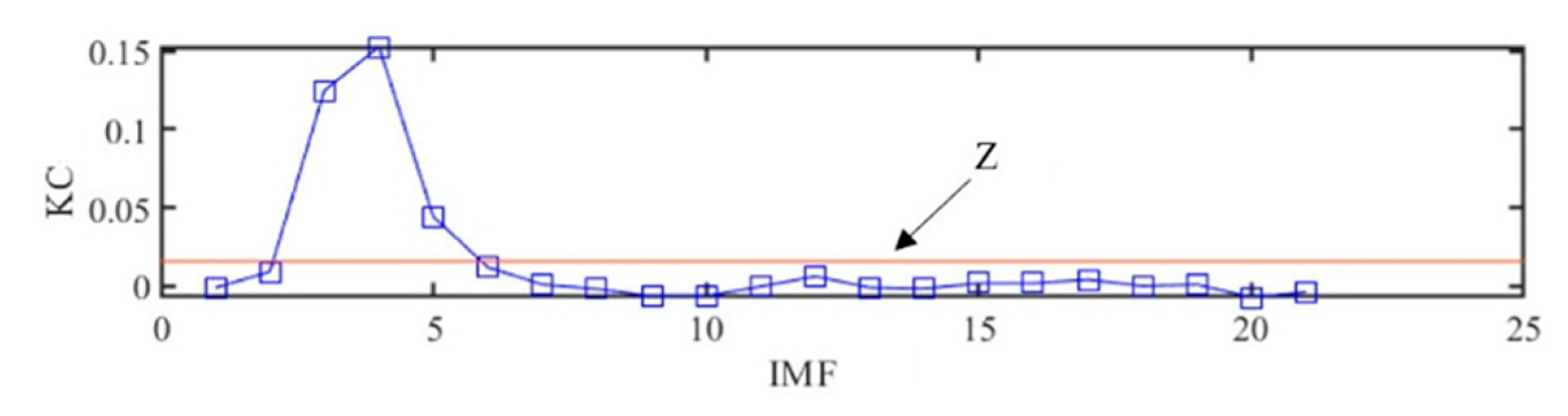
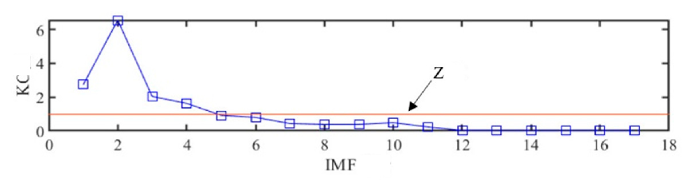
2.3. KC Indicator

Following the signal decomposition through CEEMDAN, a set of IMFs is generated. However, only a subset of these components effectively reflects the fault characteristics, and most of the others are interference components. Therefore, it is imperative to select the effective IMF components to achieve signal reconstruction [41].

Kurtosis and correlation function are widely employed indicators for the selection of effective IMF components [42,43,44,45,46]. In Ref. [47], a novel indicator that combines kurtosis and unbiased autocorrelation is introduced. However, these approaches predominantly emphasize the selection of the highest or a few relatively large values, which lacks a well-defined threshold.

Hence, a new indicator called the KC indicator is designed to take advantage of kurtosis and correlation function. Furthermore, the threshold for the selection of effective IMF components can also be defined as the average of all KC values. This averaged value is referred to as the Z value. IMF components with KC values exceeding the Z value are retained, while the others are excluded. Equations (9)–(12) are the calculation formulas for kurtosis, correlation function, KC, and Z, respectively.

$$K=\frac{{{\displaystyle \sum }}_{t=1}^N{\left[x\left(t\right)-\overline{x}\right]}^4}{{\left[{{\displaystyle \sum }}_{t=1}^N{\left[x\left(t\right)-\overline{x}\right]}^2\right]}^2},$$

(9)

$$C\left(x,IM{F}_i\right)=\frac{{{\displaystyle \sum }}_{t=1}^N\left[x\left(t\right)-\overline{x}\right]\left[IM{F}_i\left(t\right)-\overline{IM{F}_i}\right]}{\sqrt{{{\displaystyle \sum }}_{t=1}^N{\left[x\left(t\right)-\overline{x}\right]}^2}\sqrt{{{\displaystyle \sum }}_{t=1}^N{\left[IM{F}_i\left(t\right)-\overline{IM{F}_i}\right]}^2}},$$

(10)

$${(KC)}_i=K\cdot C\left(x,IM{F}_i\right),$$

(11)

$$Z=\frac{{{\displaystyle \sum }}_{n=1}^i{(KC)}_i}{i},$$

(12)

where $x\left(t\right)$ represents the original signal; $IM{F}_i\left(t\right)$ denotes the $i\mathrm{th}$ IMF component; $N$ is the length of the signal, with $\overline{x\left(t\right)}=\frac{1}{N}{{\displaystyle \sum }}_{t=1}^{N}x\left(t\right)$ and $\overline{IM{F}_i}=\frac{1}{N}{{\displaystyle \sum }}_{t=1}^{N}IM{F}_i\left(t\right)$.

2.4. An Improved TFR Demodulation Method

The wavelet basis functions significantly affect the quality of TFR demodulation analysis. The Morlet wavelet is a popular choice because of its non-orthogonal properties and good time–frequency localization. In addition, the Morlet wavelet is known for its fast convergence, which can contribute to efficient and computationally effective signal processing, especially in real-time applications [48]. Meanwhile, Morlet wavelets have been proven to be very practical in fault diagnosis of rotating machinery such as gearboxes and bearings [49]. Hence, the Morlet wavelet is adopted as the wavelet basis function of TFR in this study. It is defined as follows:

$${\psi }_{Morlet}\left(t\right)={\pi }^{-\frac{1}{4}}{e}^{i{\omega }_{0}t}{e}^{-\frac{t^2}{2}},$$

(13)

It is worth noting that the wavelet coefficients obtained by CWT are complex. This complexity allows the function to capture both magnitude and phase information, which makes it suitable for weak fault feature extraction in vibration analysis. In this study, wavelet coefficients and scale coefficients are obtained by using the cwt function in MATLAB.

The classical TFR demodulation method is also referred to as the direct TFR demodulation method. It directly sums all real wavelet coefficients in the time–frequency diagram along the frequency direction to obtain a time–frequency envelope signal for diagnosis. It is worth noting that not all wavelet coefficients contain fault information, and the phase addition in complex wavelet coefficients can mitigate the noise influence. Therefore, find the global maximum value of the signal energy intensity in the TFR, and select a continuous frequency band with an energy intensity higher than 90% of this value for filtering. An improved TFR demodulation method is proposed based on the direct TFR demodulation method. The exact steps of the proposed method are outlined as follows:

(1)

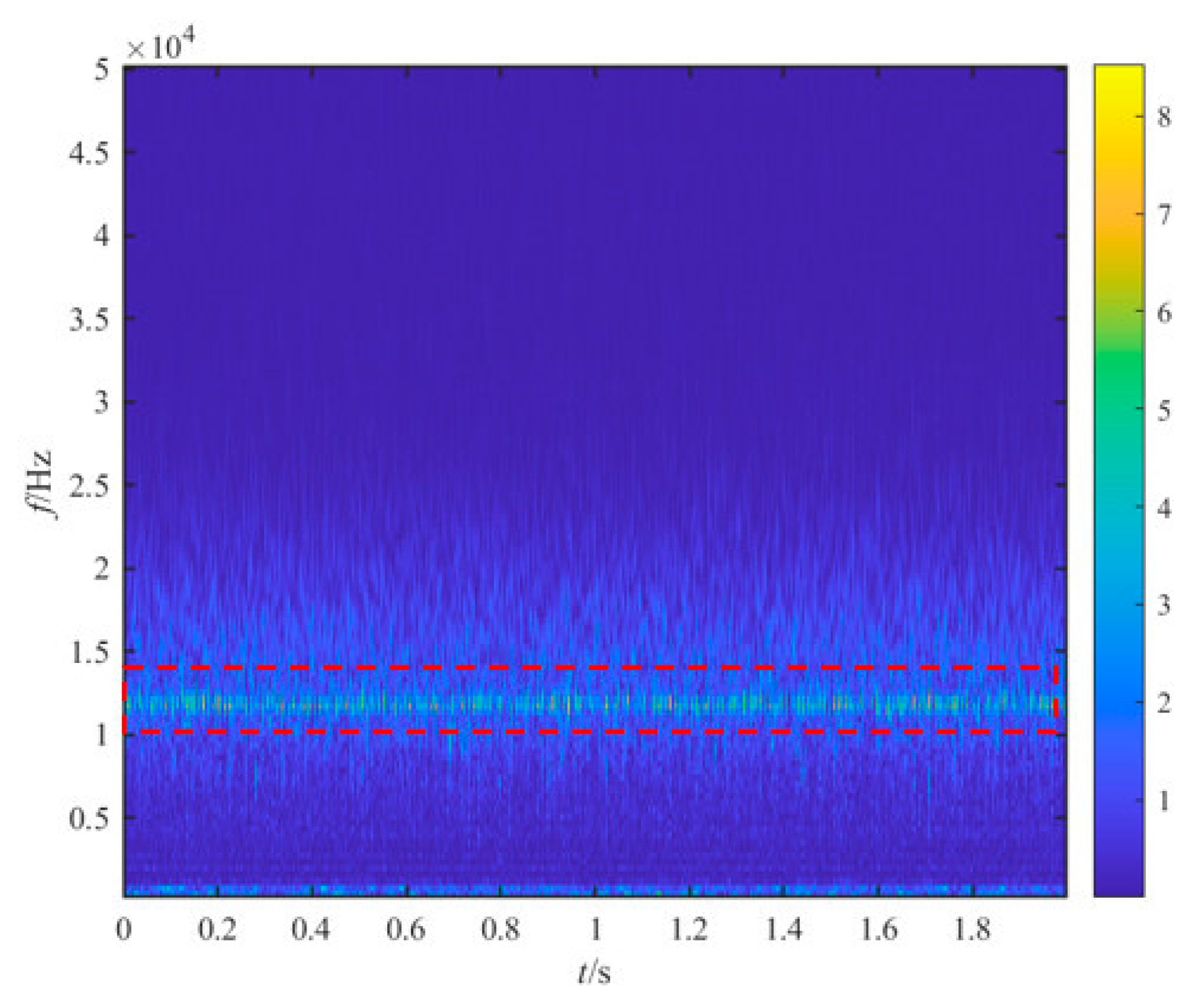
Perform CWT on the denoised signal to obtain the corresponding TFR.

(2)

Find the frequency band with the most energy concentration in the TFR. The intensity of signal energy concentration serves as the criterion for selecting a subset of wavelet coefficients.

(3)

Add the complex wavelet coefficients in the frequency band, and then calculate the modulus and convert it into a time–frequency envelope signal.

(4)

Perform FFT on the obtained signal to acquire the envelope spectrum used for fault diagnosis.

2.5. Fault Diagnosis Based on CEEMDAN and the Improved TFR Demodulation Method

In this section, a novel fault diagnosis method is proposed based on the combination of CEEMDAN and the improved TFR demodulation method. The specific process of the method is shown in Figure 2.

The proposed method involves the following steps:

(1)

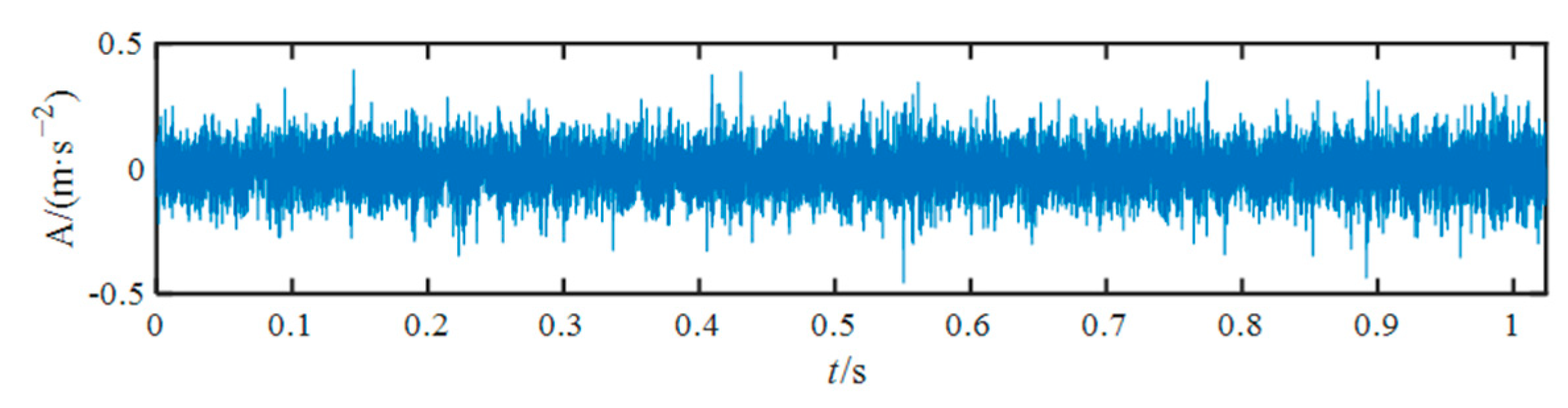
Decompose the vibration signals using CEEMDAN to obtain several IMFs.

(2)

Select the effective components based on the KC indicator to reconstruct the signal.

(3)

Perform CWT to obtain the TFR of the reconstructed signal.

(4)

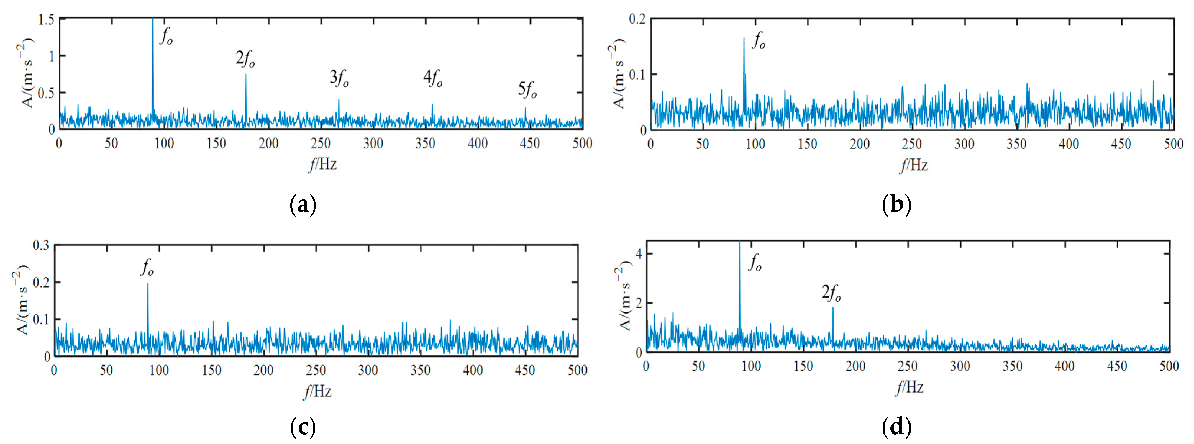
Extract the envelope spectrum using the improved TFR demodulation method.

3. Numerical Verification

Generating synthetic data is far cheaper, faster, and more convenient than collecting real data from individual machine failures [50]. In order to verify the effectiveness of the proposed method, a numerical analysis is conducted by using simulated fault signals. The vibration acceleration response of the bearing includes $2M+1$ pulses, which can be modeled as follows:

$$x\left(t\right)={{\displaystyle \sum }}_{m=-M}^M{A}_m\left(t_i\right)e^{-\beta \left(t_i\right)}\cos ({\omega }_r{t}_i)u\left(t_i\right)+n\left(t\right),$$

(14)

where $A_m$ refers to the amplitude of the $m\mathrm{th}$ defect; $M$ is the number of the shock; $u\left(t\right)$ denotes the Heaviside step function; $f_F$ indicates the FCF of the bearing; $T_0$ represents the period of the defect, with $f_F=1/T_0$; $\beta$ is the damping coefficient; ${\omega }_r$ is defined as the resonance response frequency; $n\left(t\right)$ is the Gaussian white noise; $t_i$ represents the timing of the $i\mathrm{th}$ defect, with $t_i=t-m{T}_0$.

The FCF of the bearing is 89 Hz, and the period of the simulated signal is 1/89 s. Each simulated signal consists of 285,715 data points. The sampling rate is 100 kHz and the sampling time is 2 s. Gaussian white noise is intentionally introduced to the signal. The SNR of the signal is −16 dB. Figure 3a represents the time-domain waveform of the periodically impulsive signal (the red part) with the added noise, while Figure 3b presents the envelope spectrum of the simulated signal. As can be seen from Figure 3a, the fault components are overwhelmed by noise, and the FCF cannot be accurately identified.

Further analysis is carried out by utilizing the proposed method. The simulated fault signal is decomposed by CEEMDAN, which contains 20 IMF components and 1 residual component. KC values and Z values are calculated for each IMF component. The KC values of each IMF component are presented in Figure 4.

As can be seen, substantial variations exist among the different components. Out of the 21 components examined, merely three surpassed the critical Z value. Hence, CEEMDAN effectively removes irrelevant components and enhances fault characteristics. Subsequently, those IMF components with KC values exceeding Z values (i.e., IMF3−5) are selected for reconstruction. The reconstructed signal is illustrated in Figure 5. It shows that the impulsive components are more pronounced in the signal, and noise intensity is mitigated, indicating a substantial denoising effect.

The Morlet wavelet is employed for CWT analysis on the reconstructed signal, and the corresponding TFR is obtained, as illustrated in Figure 6.

Figure 6 reveals the distribution of signal energy with various frequency bands. Subsequently, wavelet coefficients within a specific range (marked with red dot lines) are selected for addition. Their modulus is calculated to construct a time–frequency envelope signal. Subsequently, FFT is applied to generate the envelope spectrum, as shown in Figure 7a. In Figure 7, the FCF and its harmonics, namely $f_o$, $2f_o$, $3f_o$, $4f_o$, $5f_o$, are prominent, which validates the effectiveness of the proposed method.

In order to highlight the superiority of the method proposed in this article, its analysis results are compared with those of the traditional resonance demodulation method, the EMD method, and the direct TFR demodulation method.

Simulation analysis based on the traditional resonance demodulation method is conducted. The simulated signal is denoised using a bandpass filter, and then its envelope spectrum is obtained for further fault identification. The result is shown in Figure 7b. The FCF can be successfully identified, but other harmonics are difficult to observe. There are several steps to analyze the simulated signal based on the EMD method, listed as follows: firstly, the signals are decomposed by using EMD; then, the KC indicator is used to select effective IMF components for reconstruction; finally, the reconstructed signals are analyzed by using envelope spectrum. The results are shown in Figure 7c. Although the $f_o$ can be identified, other harmonics cannot be directly observed. The signals are also analyzed by using the direct TFR demodulation method, and the results are shown in Figure 7d. Although the $f_o$ and $2f_o$ can be recognized, other harmonics cannot be distinguished. As illustrated in the previous analysis, the successful recognition of the FCF harmonics and the reservation of the comprehensive fault information confirms the superiority of the proposed method.

4. Experiment Verification

In this section, two sets of experimental data will be analyzed in detail to further confirm the effectiveness of the proposed method. The experimental signals are provided by the Center for Intelligent Maintenance Systems (IMS) of the University of Cincinnati and the Case Western Reserve University (CWRU) Bearing Data Center.

4.1. REB Outer Race Fault Diagnosis

The experimental data in this section are provided by the Intelligent Maintenance Center of the University of Cincinnati [51]. These data are from bearing fatigue failure experiments conducted under constant load conditions. The experiment used four Rexnord ZA-2115 double-row cylindrical roller bearings, and each row has 16 rollers. The bearing pitch diameter is 75.5 mm, the roller diameter is 8.4 mm, and the contact angle is 15.17°. A PCB 353B33 piezoelectric accelerometer is installed on each bearing housing, and the data are collected through a DAQ-6062E data acquisition card.

There are three data sets of the entire bearing life cycle, each set containing vibration data from four bearings. The sampling rate is 20 kHz and the sampling time is 1 s. Each signal consists of 20,480 data points [52]. In this study, the vibration data of bearing 1 (outer race fault) is chosen for analysis in dataset 2. After calculation, the FCF of the bearing is determined to be 236.4 Hz. Figure 8 shows the time-domain waveform of the vibration signal.

The vibration signal is analyzed by utilizing the proposed method. The CEEMDAN decomposition is employed on the vibration signal, and the KC value and Z value of each IMF component are calculated. A graphical representation of the KC values is depicted in Figure 9.

The components whose KC values are greater than the Z value (i.e., IMF1−4) are combined into a denoised signal. Subsequently, the improved TFR demodulation method is used to analyze the denoised signal and obtain the final result.

Figure 10 shows the time–frequency diagram obtained from CWT, while Figure 11a presents the result obtained from the proposed method. It can be seen that the FCF and its harmonics are distinctly prominent and easily identifiable in the envelope spectrum. This indicates the existence of an outer race fault.

Finally, the signal is analyzed by using the traditional resonant demodulation method, the EMD analysis method, and the direct TFR demodulation method. The results are shown in Figure 11b–d. The analysis results of the four methods show that the proposed method can not only find the FCF but also emphasize its harmonics. The envelope spectrum contains more bearing fault information. Conversely, the remaining three methods solely succeed in extracting the FCF and its second-order harmonic, while struggling to extract other harmonics. Consequently, the proposed method exhibits commendable diagnostic efficiency. Hence, it can diagnose early-stage faults more effectively.

4.2. REB Inner Race Fault Diagnosis

The experimental data are provided by CWRU Bearing Data Center [53] in this section. The test rig comprises an electric motor, a torque sensor, and a force gauge. The fault with a diameter ranging from 0.007 to 0.028 inches is set on the bearing ring by using electro-discharge machining (EDM). The bearings are a type of SKF deep groove ball bearings (6205-2RS JEM and 6203-2RS JEM). In the following analysis, a vibration signal with an inner race fault will be studied. The sampling rate is 12 kHz, the rotational frequency is 29.9 Hz, and the FCF is 162.1 Hz. Figure 12 shows the time-domain waveform of the vibration signal.

The proposed method is used for analysis. The specific steps are the same as the analyzing process of simulation signals. Figure 13 illustrates the KC values for each IMF component. It can be observed that the KC values of IMF1-4 exceed the Z value; therefore these four components are chosen for signal reconstruction.

Figure 14 is the TFR diagram obtained by CWT. Figure 15a is the result obtained by using the proposed method, while Figure 15b–d exhibit the analysis results obtained by using the traditional resonance demodulation method, EMD analysis method, and direct TFR demodulation analysis method, respectively

By comparing the results of four analysis methods, the proposed method can not only find the FCF and its harmonics, but also present prominent frequency spectral lines. Although the other three methods can also find FCF, the higher harmonics in their envelope spectrum are not obvious. It can be concluded that the proposed method provides more fault information and better performance in terms of bearing fault diagnosis.

To demonstrate the effectiveness of the proposed method, the kurtosis index is used to quantify the impulsiveness of the simulation signal, outer race fault signal, and inner race fault signal respectively, as shown in Figure 16. Compared with the original signal, the kurtosis of the signal processed by the proposed method increased by 160.40%, 9.93%, and 28.86% respectively. Hence, it can be concluded that the proposed method effectively enhances the fault characteristics of the signal and suppresses the noise.

5. Conclusions

In this paper, a novel fault diagnosis method based on CEEMDAN and an improved TFR demodulation method is proposed. The purpose of the current study is to address the problem of the weak fault signals of the wind turbine rolling element bearings that are overshadowed by the noise. Firstly, the CEEMDAN method is used to decompose the signal. Secondly, a novel KC indicator is designed to select the optimal demodulation components for signal reconstruction. Finally, an improved TFR demodulation method based on CWT is applied to extract the envelope spectrum. The major advantages of the proposed method are its ability to eliminate interference noise and enhance the strength of FCF and its harmonics. The effectiveness of the proposed method is validated by the analysis of simulated signals and experimental datasets provided by the Center for Intelligent Maintenance Systems (IMS) of the University of Cincinnati and the CWRU Bearing Data Center. The traditional resonance demodulation method, EMD analysis methods, and direct TFR demodulation methods are compared with the proposed method to demonstrate its superiority. Compared with the original signal, the kurtosis of the signal processed by the proposed method increased by 160.40%, 9.93%, and 28.86%, respectively. The results show that the proposed method achieves the best outcomes in terms of noise elimination and fault feature extraction. This method exhibits notable strengths in terms of its elevated computational efficiency and practical feasibility. It is believed that the proposed method can benefit the wind energy industry by reducing downtime, minimizing maintenance costs, and improving the overall reliability of wind turbines.

References

- Chang, L.; Saydaliev, H.B.; Meo, M.S.; Mohsin, M. How Renewable Energy Matter for Environmental Sustainability: Evidence from Top-10 Wind Energy Consumer Countries of European Union. Sustain. Energy Grids Netw. 2022, 31, 100716. [Google Scholar] [CrossRef]
- Sadorsky, P. Wind Energy for Sustainable Development: Driving Factors and Future Outlook. J. Clean. Prod. 2021, 289, 125779. [Google Scholar] [CrossRef]
- Qian, P.; Feng, B.; Zhang, D.; Tian, X.; Si, Y. IoT-Based Approach to Condition Monitoring of the Wave Power Generation System. IET Renew. Power Gener. 2019, 13, 2207–2214. [Google Scholar] [CrossRef]
- McKenna, R.; Pfenninger, S.; Heinrichs, H.; Schmidt, J.; Staffell, I.; Bauer, C.; Gruber, K.; Hahmann, A.N.; Jansen, M.; Klingler, M.; et al. High-Resolution Large-Scale Onshore Wind Energy Assessments: A Review of Potential Definitions, Methodologies and Future Research Needs. Renew. Energy 2022, 182, 659–684. [Google Scholar] [CrossRef]
- Stathopoulos, T.; Alrawashdeh, H.; Al-Quraan, A.; Blocken, B.; Dilimulati, A.; Paraschivoiu, M.; Pilay, P. Urban Wind Energy: Some Views on Potential and Challenges. J. Wind Eng. Ind. Aerodyn. 2018, 179, 146–157. [Google Scholar] [CrossRef]
- Soua, S.; Van Lieshout, P.; Perera, A.; Gan, T.-H.; Bridge, B. Determination of the Combined Vibrational and Acoustic Emission Signature of a Wind Turbine Gearbox and Generator Shaft in Service as a Pre-Requisite for Effective Condition Monitoring. Renew. Energy 2013, 51, 175–181. [Google Scholar] [CrossRef]
- Dhanola, A.; Garg, H.C. Tribological Challenges and Advancements in Wind Turbine Bearings: A Review. Eng. Fail. Anal. 2020, 118, 104885. [Google Scholar] [CrossRef]
- Wang, J.; Liang, Y.; Zheng, Y.; Gao, R.X.; Zhang, F. An Integrated Fault Diagnosis and Prognosis Approach for Predictive Maintenance of Wind Turbine Bearing with Limited Samples. Renew. Energy 2020, 145, 642–650. [Google Scholar] [CrossRef]
- De Azevedo, H.D.M.; Araújo, A.M.; Bouchonneau, N. A Review of Wind Turbine Bearing Condition Monitoring: State of the Art and Challenges. Renew. Sustain. Energy Rev. 2016, 56, 368–379. [Google Scholar] [CrossRef]
- Fischer, K.; Besnard, F.; Bertling, L. Reliability-Centered Maintenance for Wind Turbines Based on Statistical Analysis and Practical Experience. IEEE Trans. Energy Convers. 2012, 27, 184–195. [Google Scholar] [CrossRef]
- Qian, P.; Zhang, D.; Tian, X.; Si, Y.; Li, L. A Novel Wind Turbine Condition Monitoring Method Based on Cloud Computing. Renew. Energy 2019, 135, 390–398. [Google Scholar] [CrossRef]
- Qian, P.; Ma, X.; Zhang, D.; Wang, J. Data-Driven Condition Monitoring Approaches to Improving Power Output of Wind Turbines. IEEE Trans. Ind. Electron. 2019, 66, 6012–6020. [Google Scholar] [CrossRef]
- Liu, Z.; Zhang, L. A Review of Failure Modes, Condition Monitoring and Fault Diagnosis Methods for Large-Scale Wind Turbine Bearings. Measurement 2020, 149, 107002. [Google Scholar] [CrossRef]
- Liu, L.; Wei, Y.; Song, X.; Zhang, L. Fault Diagnosis of Wind Turbine Bearings Based on CEEMDAN-GWO-KELM. Energies 2022, 16, 48. [Google Scholar] [CrossRef]
- Hu, Y.; Zhang, S.; Jiang, A.; Zhang, L.; Jiang, W.; Li, J. A New Method of Wind Turbine Bearing Fault Diagnosis Based on Multi-Masking Empirical Mode Decomposition and Fuzzy C-Means Clustering. Chin. J. Mech. Eng. 2019, 32, 46. [Google Scholar] [CrossRef]
- Randall, R.B.; Antoni, J. Rolling Element Bearing Diagnostics—A Tutorial. Mech. Syst. Signal Process. 2011, 25, 485–520. [Google Scholar] [CrossRef]
- Zhou, J.; Chen, C.; Guo, J.; Wang, L.; Liu, Z.; Feng, C. A Novel Rolling Bearing Fault Diagnosis Method Based on Continuous Hierarchical Fractional Range Entropy. Measurement 2023, 220, 113395. [Google Scholar] [CrossRef]
- Pang, B.; Nazari, M.; Tang, G. Recursive Variational Mode Extraction and Its Application in Rolling Bearing Fault Diagnosis. Mech. Syst. Signal Process. 2022, 165, 108321. [Google Scholar] [CrossRef]
- Xu, Y.; Li, Z.; Wang, S.; Li, W.; Sarkodie-Gyan, T.; Feng, S. A Hybrid Deep-Learning Model for Fault Diagnosis of Rolling Bearings. Measurement 2021, 169, 108502. [Google Scholar] [CrossRef]
- Wang, J.; Mo, Z.; Zhang, H.; Miao, Q. A Deep Learning Method for Bearing Fault Diagnosis Based on Time-Frequency Image. IEEE Access 2019, 7, 42373–42383. [Google Scholar] [CrossRef]
- Saucedo-Dorantes, J.J.; Arellano-Espitia, F.; Delgado-Prieto, M.; Osornio-Rios, R.A. Diagnosis Methodology Based on Deep Feature Learning for Fault Identification in Metallic, Hybrid and Ceramic Bearings. Sensors 2021, 21, 5832. [Google Scholar] [CrossRef]
- Cristescu, N.D.; Craciun, E.-M.; Gaunaurd, G.C. Mechanics of Elastic Composites (CRC Series in Modern Mechanics and Mathematics). Appl. Mech. Rev. 2004, 57, B27. [Google Scholar] [CrossRef]
- Li, Y.; Wang, J.; Feng, D.; Jiang, M.; Peng, C.; Geng, X.; Zhang, F. Bearing Fault Diagnosis Method Based on Maximum Noise Ratio Kurtosis Product Deconvolution with Noise Conditions. Measurement 2023, 221, 113542. [Google Scholar] [CrossRef]
- Wang, Q.; Xu, F. A Novel Rolling Bearing Fault Diagnosis Method Based on Adaptive Denoising Convolutional Neural Network under Noise Background. Measurement 2023, 218, 113209. [Google Scholar] [CrossRef]
- Yin, C.; Wang, Y.; Ma, G.; Wang, Y.; Sun, Y.; He, Y. Weak Fault Feature Extraction of Rolling Bearings Based on Improved Ensemble Noise-Reconstructed EMD and Adaptive Threshold Denoising. Mech. Syst. Signal Process. 2022, 171, 108834. [Google Scholar] [CrossRef]
- Kedadouche, M.; Thomas, M.; Tahan, A. A Comparative Study between Empirical Wavelet Transforms and Empirical Mode Decomposition Methods: Application to Bearing Defect Diagnosis. Mech. Syst. Signal Process. 2016, 81, 88–107. [Google Scholar] [CrossRef]
- Huang, N.E.; Shen, Z.; Long, S.R.; Wu, M.C.; Shih, H.H.; Zheng, Q.; Yen, N.-C.; Tung, C.C.; Liu, H.H. The Empirical Mode Decomposition and the Hilbert Spectrum for Nonlinear and Non-Stationary Time Series Analysis. Proc. R. Soc. London. Ser. A Math. Phys. Eng. Sci. 1998, 454, 903–995. [Google Scholar] [CrossRef]
- Tian, S.; Bian, X.; Tang, Z.; Yang, K.; Li, L. Fault Diagnosis of Gas Pressure Regulators Based on CEEMDAN and Feature Clustering. IEEE Access 2019, 7, 132492–132502. [Google Scholar] [CrossRef]
- Wu, Z.; Huang, N.E. Ensemble Empirical Mode Decomposition: A Noise-Assisted Data Analysis Method. Adv. Adapt. Data Anal. 2009, 1, 1–41. [Google Scholar] [CrossRef]
- Torres, M.E.; Colominas, M.A.; Schlotthauer, G.; Flandrin, P. A Complete Ensemble Empirical Mode Decomposition with Adaptive Noise. In Proceedings of the 2011 IEEE International Conference on Acoustics, Speech and Signal Processing (ICASSP), Toronto, ON, Canada, 22–27 May 2011; pp. 4144–4147. [Google Scholar]
- Cheng, Y.; Wang, Z.; Chen, B.; Zhang, W.; Huang, G. An Improved Complementary Ensemble Empirical Mode Decomposition with Adaptive Noise and Its Application to Rolling Element Bearing Fault Diagnosis. ISA Trans. 2019, 91, 218–234. [Google Scholar] [CrossRef]
- Yang, Y.; Li, S.; Li, C.; He, H.; Zhang, Q. Research on Ultrasonic Signal Processing Algorithm Based on CEEMDAN Joint Wavelet Packet Thresholding. Measurement 2022, 201, 111751. [Google Scholar] [CrossRef]
- Zhou, H.; Yan, P.; Yuan, Y.; Wu, D.; Huang, Q. Denoising the Hob Vibration Signal Using Improved Complete Ensemble Empirical Mode Decomposition with Adaptive Noise and Noise Quantization Strategies. ISA Trans. 2022, 131, 715–735. [Google Scholar] [CrossRef] [PubMed]
- Qian, P.; Tian, X.; Kanfoud, J.; Lee, J.; Gan, T.-H. A Novel Condition Monitoring Method of Wind Turbines Based on Long Short-Term Memory Neural Network. Energies 2019, 12, 3411. [Google Scholar] [CrossRef]
- Zhang, X.; Wan, S.; He, Y.; Wang, X.; Dou, L. Teager Energy Spectral Kurtosis of Wavelet Packet Transform and Its Application in Locating the Sound Source of Fault Bearing of Belt Conveyor. Measurement 2021, 173, 108367. [Google Scholar] [CrossRef]
- Han, T.; Liu, Q.; Zhang, L.; Tan, A.C.C. Fault Feature Extraction of Low Speed Roller Bearing Based on Teager Energy Operator and CEEMD. Measurement 2019, 138, 400–408. [Google Scholar] [CrossRef]
- Wang, L.; Shao, Y. Fault Feature Extraction of Rotating Machinery Using a Reweighted Complete Ensemble Empirical Mode Decomposition with Adaptive Noise and Demodulation Analysis. Mech. Syst. Signal Process. 2020, 138, 106545. [Google Scholar] [CrossRef]
- Chen, W.; Li, J.; Wang, Q.; Han, K. Fault Feature Extraction and Diagnosis of Rolling Bearings Based on Wavelet Thresholding Denoising with CEEMDAN Energy Entropy and PSO-LSSVM. Measurement 2021, 172, 108901. [Google Scholar] [CrossRef]
- Sun, H.; He, Z.; Zi, Y.; Yuan, J.; Wang, X.; Chen, J.; He, S. Multiwavelet Transform and Its Applications in Mechanical Fault Diagnosis—A Review. Mech. Syst. Signal Process. 2014, 43, 1–24. [Google Scholar] [CrossRef]
- Zhan, Y.; Halliday, D.; Jiang, P.; Liu, X.; Feng, J. Detecting Time-Dependent Coherence between Non-Stationary Electrophysiological Signals—A Combined Statistical and Time–Frequency Approach. J. Neurosci. Methods 2006, 156, 322–332. [Google Scholar] [CrossRef]
- Zhou, S.; Zhang, Z.-X.; Luo, X.; Niu, S.; Jiang, N.; Yao, Y. Developing a Hybrid CEEMDAN-PE-HE-SWT Method to Remove the Noise of Measured Carbon Dioxide Blast Wave. Measurement 2023, 223, 113797. [Google Scholar] [CrossRef]
- Antoni, J. The Spectral Kurtosis: A Useful Tool for Characterising Non-Stationary Signals. Mech. Syst. Signal Process. 2006, 20, 282–307. [Google Scholar] [CrossRef]
- Antoni, J. Fast Computation of the Kurtogram for the Detection of Transient Faults. Mech. Syst. Signal Process. 2007, 21, 108–124. [Google Scholar] [CrossRef]
- Antoni, J. Cyclostationarity by Examples. Mech. Syst. Signal Process. 2009, 23, 987–1036. [Google Scholar] [CrossRef]
- Gardner, W.A. The Spectral Correlation Theory of Cyclostationary Time-Series. Signal Process. 1986, 11, 13–36. [Google Scholar] [CrossRef]
- Randall, R.B.; Antoni, J.; Chobsaard, S. The Relationship between Spectral Correlation and Envelope Analysis in The Diagnostics of Bearing Faults and Other Cyclostationary Machine Signals. Mech. Syst. Signal Process. 2001, 15, 945–962. [Google Scholar] [CrossRef]
- Moshrefzadeh, A.; Fasana, A. The Autogram: An Effective Approach for Selecting the Optimal Demodulation Band in Rolling Element Bearings Diagnosis. Mech. Syst. Signal Process. 2018, 105, 294–318. [Google Scholar] [CrossRef]
- Sheen, Y.-T.; Hung, C.-K. Constructing a Wavelet-Based Envelope Function for Vibration Signal Analysis. Mech. Syst. Signal Process. 2004, 18, 119–126. [Google Scholar] [CrossRef]
- Tian, X.; Xi Gu, J.; Rehab, I.; Abdalla, G.M.; Gu, F.; Ball, A.D. A Robust Detector for Rolling Element Bearing Condition Monitoring Based on the Modulation Signal Bispectrum and Its Performance Evaluation against the Kurtogram. Mech. Syst. Signal Process. 2018, 100, 167–187. [Google Scholar] [CrossRef]
- Jablonski, A. Hybrid Model of Rolling-Element Bearing Vibration Signal. Energies 2022, 15, 4819. [Google Scholar] [CrossRef]
- Qiu, H.; Lee, J.; Lin, J.; Yu, G. Wavelet Filter-Based Weak Signature Detection Method and Its Application on Rolling Element Bearing Prognostics. J. Sound Vib. 2006, 289, 1066–1090. [Google Scholar] [CrossRef]
- Gousseau, W.; Antoni, J.; Girardin, F.; Lyon, U.; Griffaton, J. Analysis of the Rolling Element Bearing Data Set of the Center for Intelligent Maintenance Systems of the University of Cincinnati. In Proceedings of the CM2016, Charenton, France, 10–12 October 2016. [Google Scholar]
- Smith, W.A.; Randall, R.B. Rolling Element Bearing Diagnostics Using the Case Western Reserve University Data: A Benchmark Study. Mech. Syst. Signal Process. 2015, 64–65, 100–131. [Google Scholar] [CrossRef]
Disclaimer/Publisher’s Note: The statements, opinions and data contained in all publications are solely those of the individual author(s) and contributor(s) and not of MDPI and/or the editor(s). MDPI and/or the editor(s) disclaim responsibility for any injury to people or property resulting from any ideas, methods, instructions or products referred to in the content. |
© 2024 by the authors. Licensee MDPI, Basel, Switzerland. This article is an open access article distributed under the terms and conditions of the Creative Commons Attribution (CC BY) license (https://creativecommons.org/licenses/by/4.0/).
Share and Cite
Zhang, D.; Wang, Y.; Jiang, Y.; Zhao, T.; Xu, H.; Qian, P.; Li, C. A Novel Wind Turbine Rolling Element Bearing Fault Diagnosis Method Based on CEEMDAN and Improved TFR Demodulation Analysis. Energies 2024, 17, 819. https://doi.org/10.3390/en17040819
Zhang D, Wang Y, Jiang Y, Zhao T, Xu H, Qian P, Li C. A Novel Wind Turbine Rolling Element Bearing Fault Diagnosis Method Based on CEEMDAN and Improved TFR Demodulation Analysis. Energies. 2024; 17(4):819. https://doi.org/10.3390/en17040819
Chicago/Turabian StyleZhang, Dahai, Yiming Wang, Yongjian Jiang, Tao Zhao, Haiyang Xu, Peng Qian, and Chenglong Li. 2024. "A Novel Wind Turbine Rolling Element Bearing Fault Diagnosis Method Based on CEEMDAN and Improved TFR Demodulation Analysis" Energies 17, no. 4: 819. https://doi.org/10.3390/en17040819
APA StyleZhang, D., Wang, Y., Jiang, Y., Zhao, T., Xu, H., Qian, P., & Li, C. (2024). A Novel Wind Turbine Rolling Element Bearing Fault Diagnosis Method Based on CEEMDAN and Improved TFR Demodulation Analysis. Energies, 17(4), 819. https://doi.org/10.3390/en17040819