A Novel Data-Driven Approach for Predicting the Performance Degradation of a Gas Turbine

Abstract

Gas turbines operate under harsh conditions of high temperature and pressure for extended periods, inevitably experiencing performance degradation. Predicting the performance degradation trend of gas turbines and optimizing planned maintenance cycles are crucial for the economic and safety aspects of gas turbine operation. In this study, a novel data-driven approach for predicting gas turbine performance degradation is proposed. Initially, gas turbine operating data are augmented using a mechanism model. Subsequently, a data-driven performance model is constructed based on support vector regression (SVR) and gas turbine operational characteristics, enabling real-time calculation of performance degradation indicators. Building on this, an Autoregressive Neural Network (AR-Net) is employed to construct a model for predicting the trend of performance degradation. The proposed method is applied to predict performance degradation caused by fouling in the compressor of a gas turbine. Comparative analysis with three other performance degradation prediction methods indicates that the proposed approach accurately identifies the performance degradation trend of gas turbines, determining the optimal maintenance timing. This holds significant importance for the condition-based maintenance of gas turbines.

1. Introduction

Gas turbines are advanced power equipment with high energy efficiency, strong fuel adaptability, and low pollutant emissions, making them important for constructing clean, low-carbon, safe, and efficient energy systems. However, operating consistently under harsh conditions of high temperature, high pressure, and polluted environments, gas turbines experience varying forms and degrees of performance degradation. This degradation leads to a decline in the thermal efficiency and output power of gas turbines, thereby impacting the economic viability and safety of gas turbine power plants [1]. Common causes of performance degradation in gas turbines include fouling, wear, erosion, corrosion, and increased blade tip clearances [2]. Among these, fouling is the most prevalent degradation mode, with compressor fouling typically accounting for approximately 70–85% of the total performance loss [3]. This is because gas turbines intake a large volume of air, inevitably introducing dust, sand, salt, and other impurities from the air, leading to adverse effects, such as reduced efficiency and flow in the compressor [4].

In the operation and maintenance process of industrial gas turbines, regular water washing strategies are commonly employed to remove compressor fouling. Among them, online water washing does not require shutdown but has relatively poorer effectiveness, while offline water washing is more thorough compared to online water washing and can effectively eliminate the impact of compressor fouling. However, the disadvantage is that it requires a shutdown [5]. Therefore, optimizing the water washing cycle, that is, the interval for offline water washing, is crucial during the operation of the gas turbine. If the water washing cycle is too short, the cost of shutdown and offline washing becomes prohibitively high. Conversely, an extended cycle may result in a significant reduction in gas turbine output power due to compressor fouling, subsequently increasing the cost of electricity generation and potentially compromising the safety of the gas turbine.

In order to predict the performance degradation trend of gas turbines, it is essential to first establish a performance model for the gas turbine under healthy conditions. This model should reflect the output parameters of the gas turbine under different environmental and control conditions and then be used to calculate the differences between actual performance parameters and healthy state performance parameters [6]. The most common approach involves the use of physics-based methods, which utilize mechanism models to calculate the health parameters of the gas turbine. This includes nonlinear Gas Path Analysis (GPA) methods [7,8], Kalman Filtering algorithms, and their variations [9,10].

Due to the drawbacks of physical models, such as computational complexity and the need for accurate component characteristic curves, data-driven models have gained significant attention. The main data-driven models include artificial neural networks (ANNs) [11,12], XGBoost [13], high-dimensional model representation (HDMR) [14], etc. Data-driven models, once trained, have significantly lower computational costs compared to physics-based models. Sometimes, even when physics-based models are available, data-driven models may be trained using simulated data generated by the physics-based model [15]. Therefore, data-driven models, characterized by their speed and adaptability, have broad application prospects.

The prediction of performance degradation in gas turbines aims to forecast the development trend of performance parameters over a period of time. By predicting the performance degradation before it reaches a predetermined threshold, appropriate maintenance measures can be scheduled while avoiding unexpected failures [6]. Y.G. Li et al. [16] proposed a hybrid model combining linear regression and quadratic regression to predict the remaining service life of gas turbine engines. Based on real-time operational data, the corresponding regression model is selected, and coefficients are determined. Zhou Dengji et al. [17], taking into account the uncertainty of performance degradation data and the requirement for long-term prediction, proposed a gray prediction model based on Markov processes and gray correlation analysis. Using the fouling process of a gas turbine compressor as an example, they demonstrated that this model outperforms other prediction models. However, this method requires performance degradation data from multiple gas turbines with different models. Wang Weiying et al. [18] presented a gas turbine air path performance degradation prediction method based on the ARIMA time series model. Through simulation experiments, it was proven effective in predicting the degradation trend caused by the compressor fouling. However, this method is only suitable for short-term prediction, and its long-term prediction performance is poor. Marta Zagorowska et al. [19] employed a combined method of a moving window approach and adaptive regression analysis to predict the expected value of performance degradation indicators and quantify the uncertainty of the prediction. The essence of this method is to determine whether the trend of data within the moving window follows a linear or nonlinear regression and then estimate the parameters of the regression function to achieve adaptive prediction. Jinwei Chen et al. [20] proposed a sliding window prediction method based on LSTM to predict nonlinear fouling trends and identify declines in compressor flow rate and efficiency. Real field data from a gas turbine power plant were used for training and testing, and it was found that this method had a smaller relative mean square error compared to other prediction methods. Y. Jin et al. [21] developed a hybrid framework that integrates thermodynamic models and Long Short-Term Memory (LSTM) neural networks to predict washing cycles (remaining service life prediction) and detect filter leakage (filter diagnosis). The prediction model based on the LSTM–Hankel method exhibited good performance in long-term washing cycle prediction.

In neural network prediction algorithms, the Autoregressive Neural Network (AR-Net) [22] has been successfully applied to time series forecasting in various fields [23,24,25], making it a feasible method for predicting the performance degradation trend of gas turbines. This paper proposes a hybrid model-based prediction method for gas turbine performance degradation using support vector regression (SVR) and AR-Net. The method first utilizes mechanism models to augment the operating data and then constructs a performance model based on SVR and gas turbine operational characteristics. This model enables real-time estimation of performance degradation indicators. Based on the degradation indicators from historical maintenance cycles, an AR-Net prediction model is built to forecast the performance degradation trend.

The contributions of this work include the following:

(a) Proposing a novel data-driven method for predicting the performance degradation of gas turbines. Using actual operating data and augmented data generated from the mechanism model, a high-accuracy performance model under healthy conditions of gas turbines is established.

(b) Introducing the use of an Autoregressive Neural Network (AR-Net) for predicting the performance degradation trend of gas turbines. This approach can effectively utilize operating data from historical maintenance cycles.

(c) Simulating real fouling data of the compressor and comparing the predictive results of the proposed method with three other methods. The results demonstrate that the proposed method can effectively predict the offline water wash cycle of gas turbines, providing guidance for the condition-based maintenance of gas turbines.

The structure of the remaining parts of this paper is as follows. Section 2 presents a gas turbine performance degradation prediction method based on a hybrid model of SVR and AR-Net. Section 3 is the results and discussion, which first constructs the SVR performance model under healthy conditions and then calculates the performance degradation indicators in real-time for the performance degradation caused by compressor fouling and builds the AR-Net prediction model for performance degradation trend prediction. Section 4 concludes the paper.

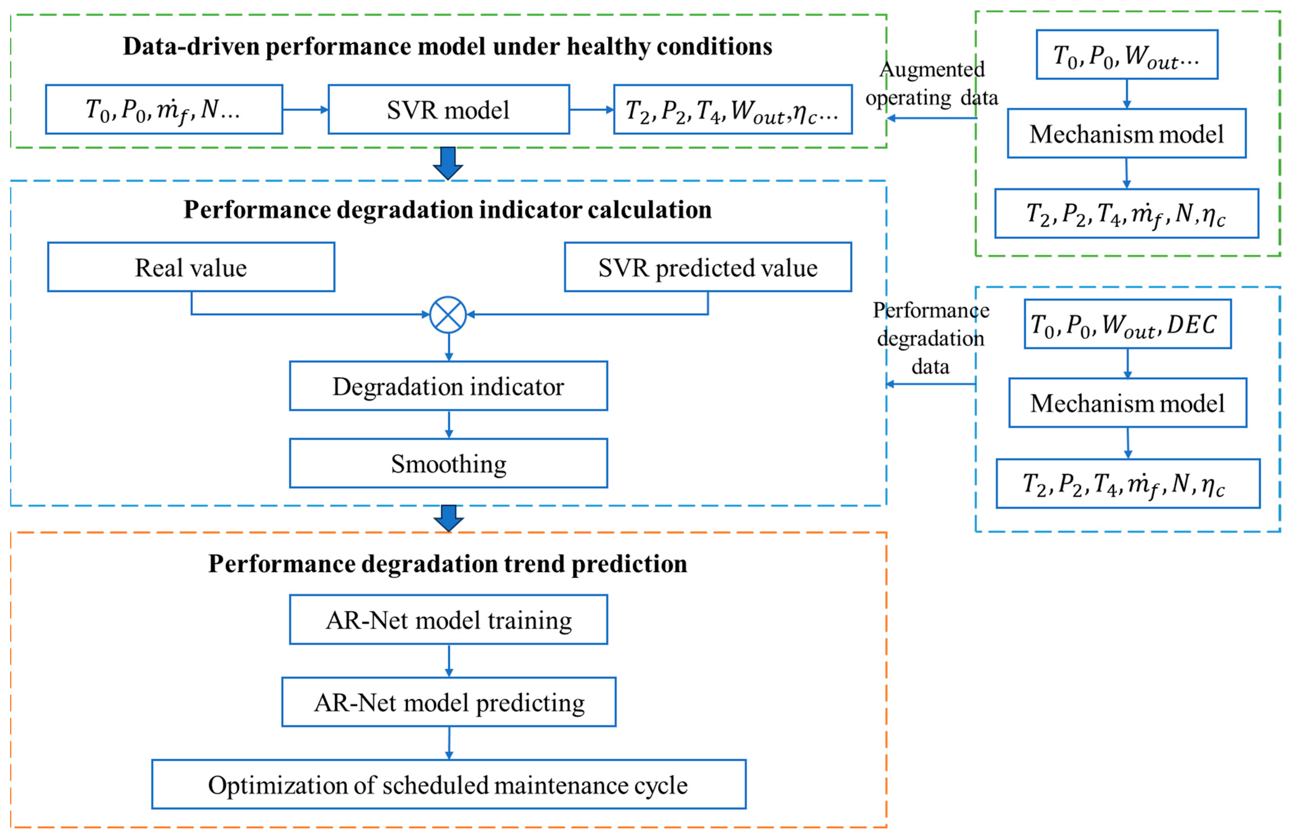
2. Methodology

The gas turbine performance degradation prediction method proposed in this paper consists of three parts: a data-driven performance model under healthy conditions, performance degradation indicator calculation, and performance degradation trend prediction. Firstly, the data-driven performance model is constructed based on the SVR algorithm. To solve the problem of insufficient actual operating data, a mechanism model is used to augment the operating data. Secondly, indicators closely related to gas turbine performance are selected, and the residual between the output value of the performance model and the real-time calculated value is calculated to obtain the performance degradation indicator. A piecewise linear function is used to smooth the degradation indicator. Finally, based on AR-Net, a trend prediction model is built to predict the performance degradation trend for a future period by learning the performance degradation trend of historical maintenance cycles. A flowchart of the proposed method is shown in Figure 1.

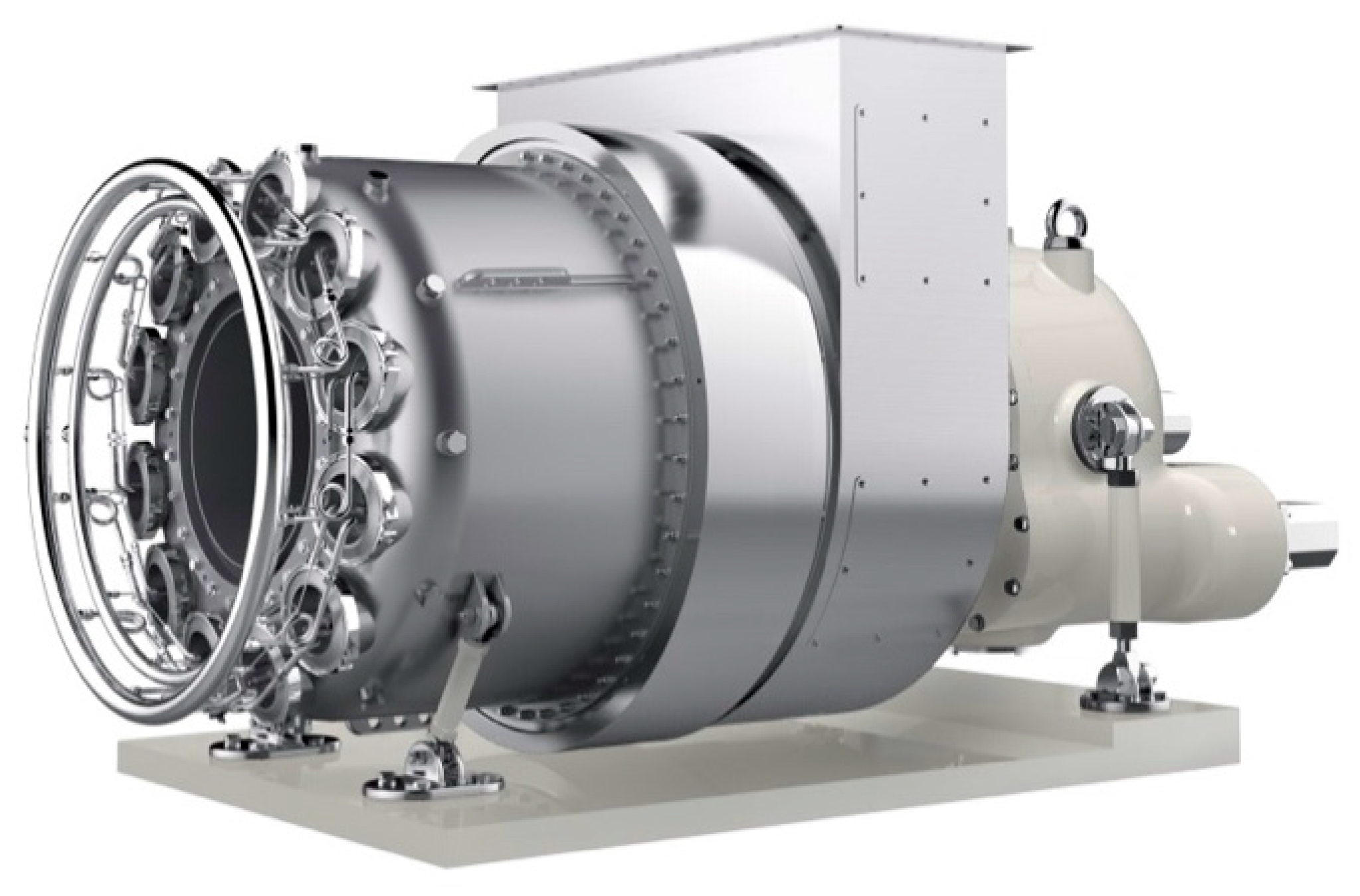
2.1. Gas Turbine Structure and Mechanism Model

The analysis target is a micro gas turbine, mainly used for industrial distributed power generation, commercial distributed power generation, mobile emergency power supply, etc. Its structure is shown in Figure 2, mainly including a single-stage centrifugal compressor, an annular combustion chamber, and a single-stage radial inflow turbine. The design point performance parameters under ISO conditions are shown in

Table 1. Performance of the gas turbine at the design point.

Parameter	Value
Power generation/MW	2
Power generation efficiency/%	25.7
Pressure ratio	7.5
Exhaust flow rate/(Kg/s)	10.1
Turbine inlet temperature/K	1223
Exhaust temperature/K	803

.

A mechanism model is established on the Matlab/Simulink platform for this gas turbine. The modules of the mechanism model are shown in Figure 3. The mechanism model can generate operating data of the gas turbine under different conditions, thereby solving the issue of insufficient training data required for the data-driven model of the gas turbine.

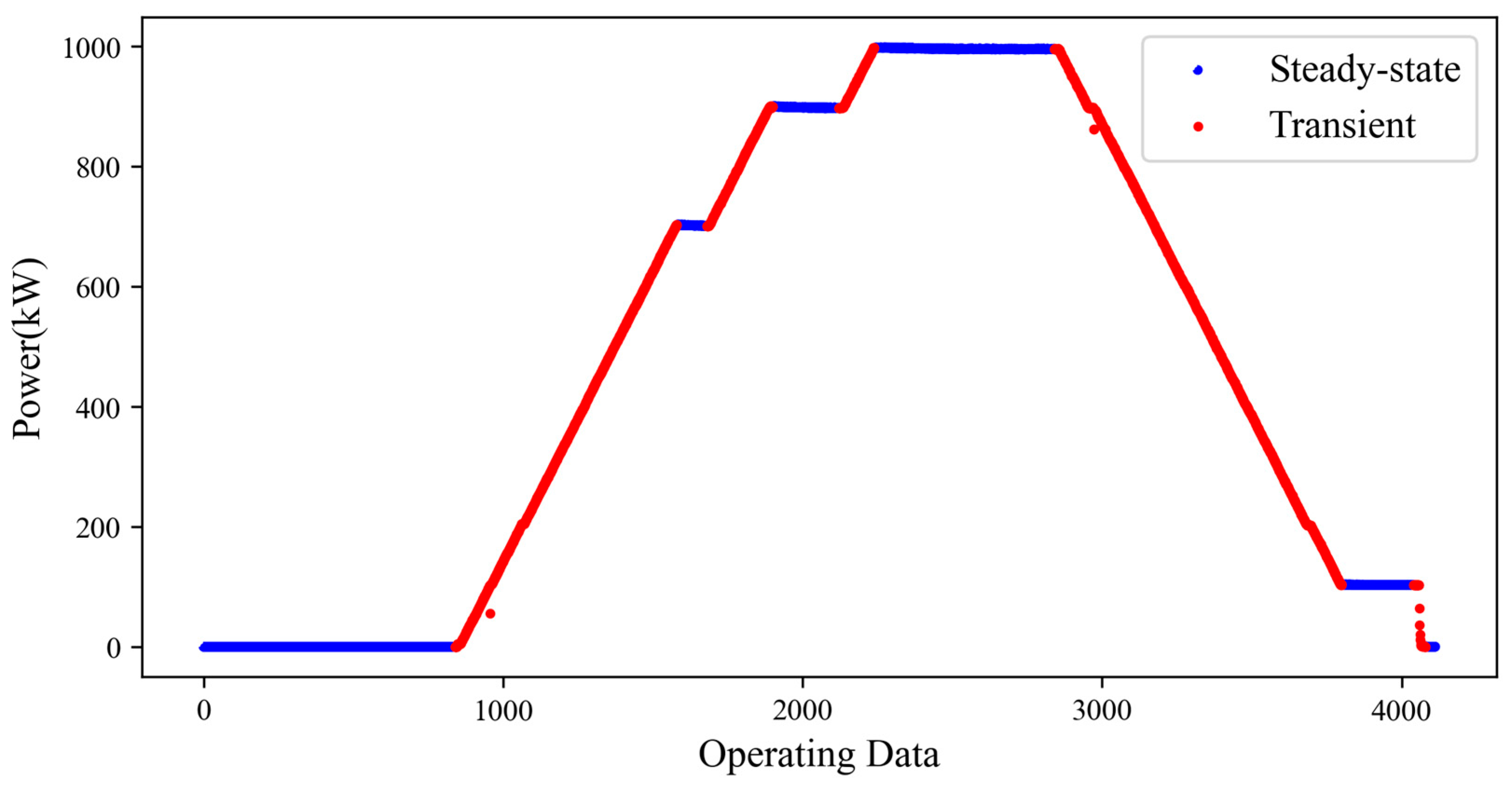
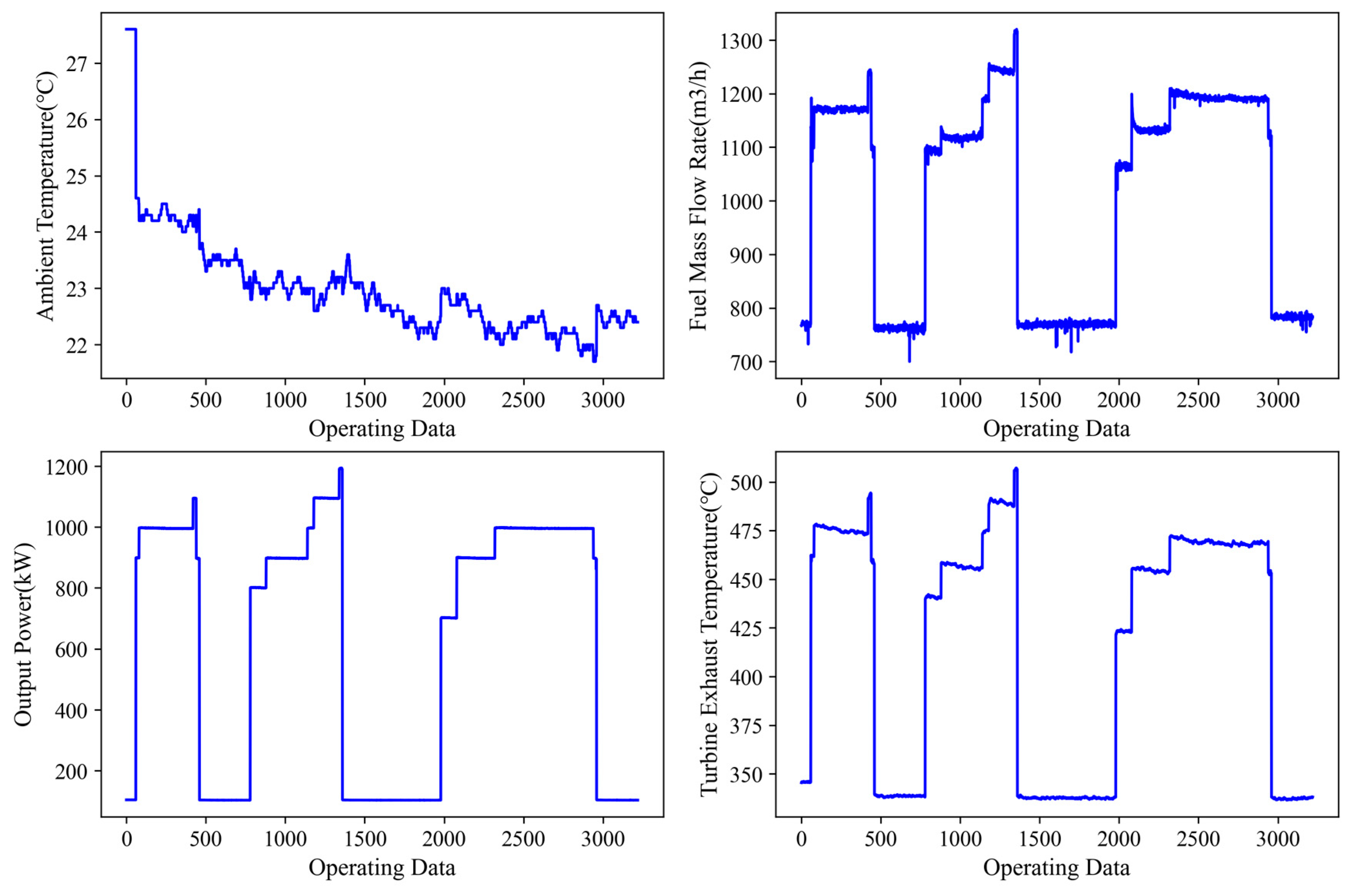
2.2. Data Preprocessing

Due to equipment failures, sensor errors, operational mistakes, and other external factors, gas turbine data often contain missing values and outliers. This can have a significant negative impact on subsequent data analysis and model development. Therefore, it is essential to first handle missing values and outliers in operational data to ensure data quality and completeness.

Considering the need for the rapid adjustment of fuel supply to meet load dispatch requirements after gas turbines are connected to the grid, there are two types of actual operating data: steady-state and transient. In this study, the performance degradation prediction is mainly based on steady-state data. Therefore, it is necessary to screen the actual operating data for steady-state conditions. This study adopts the steady-state screening algorithm proposed by Wang Zhong [26], with output power as the feature variable for steady-state filtering. The operating parameters of the gas turbine can be considered as a combination of true values and noise values. When the gas turbine is in a steady-state condition, the true values of the operating parameters remain constant, and the variations in the measured values are mainly caused by random errors. When the gas turbine is in a transient state, the true values of the operating parameters undergo significant changes, which are generally visually reflected in the changes in output power, increasing or decreasing over time. Therefore, considering the selection of output power as the feature variable for steady-state filtering, its expression is as follows:

$$p_t=\mu +mt+\epsilon \to \left\{\begin{array}{l}m=0\hspace{0.25em}\hspace{0.25em}\hspace{0.25em}\hspace{0.25em}\mathrm{s}\mathrm{t}\mathrm{e}\mathrm{a}\mathrm{d}\mathrm{y}\text{-}\mathrm{s}\mathrm{t}\mathrm{a}\mathrm{t}\mathrm{e}\\ m\ne 0\hspace{0.25em}\hspace{0.25em}\hspace{0.25em}\hspace{0.25em}\mathrm{t}\mathrm{r}\mathrm{a}\mathrm{n}\mathrm{s}\mathrm{i}\mathrm{e}\mathrm{n}\mathrm{t} \end{array}\right.$$

(1)

where $p_t$ represents the measured power at time $t$; $\mu$ represents the true value of power; $m$ represents the rate of change of power; and $\epsilon$ represents the random error of power, which follows a normal distribution.

In Equation (1), it can be seen that the difference between steady-state and transient operating conditions lies in whether the rate of power change $m$ is equal to zero. To facilitate the estimation of the $m$, the difference between the power at two consecutive time points, denoted as $\Delta p$, its expression is as follows:

$$\Delta p=p_t-p_{t-1}=m+({\epsilon }_t-{\epsilon }_{t-1})$$

(2)

As the random error $\epsilon$ follows a normal distribution, the expected value of the statistic $\Delta p$ is equal to $m$. According to the nature of time series, $m$ can be estimated using the mean of sample statistics within a time window, as shown below:

$$\widehat{m}=\stackrel{—}{\Delta p}=\frac{1}{h}\sum _{t=1}^{t=h} (p_t-p_{t-1})$$

(3)

where $h$ is the number of samples within the sampling time window.

In order to ensure the reliability of the estimation, an interval estimation method is used to determine the expected value $m$ of the sample power difference. If the estimated interval range includes 0, it is considered highly likely that the gas turbine is operating under steady-state conditions during that time period; otherwise, it is considered to be operating under transient conditions.

After obtaining steady-state operating data using the above method, in order to avoid the influence of dimensional differences between the operating data on the training of the SVR model, it is necessary to normalize the data, making it fall within the range of [0, 1]. The transformation function is as follows:

$$x_{\mathrm{n}\mathrm{o}\mathrm{r}\mathrm{m}}=\frac{x-min\left(x\right)}{max\left(x\right)-min\left(x\right)}$$

(4)

where $x_{\mathrm{n}\mathrm{o}\mathrm{r}\mathrm{m}}$ is the normalized value, $min\left(x\right)$ is the minimum value of $x$, and $max\left(x\right)$ is the maximum value of $x$.

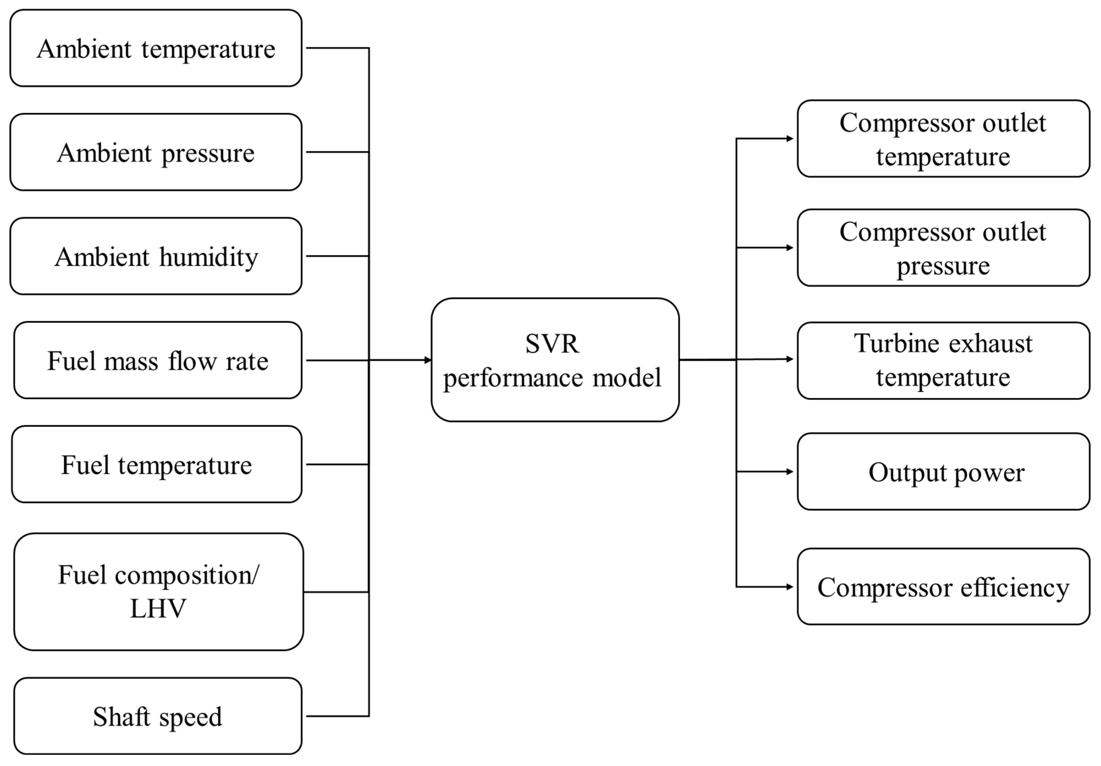
2.3. Gas Turbine Performance Model Based on Support Vector Regression

Support vector regression (SVR) [27] is a nonlinear supervised learning algorithm that is suitable for solving high-dimensional pattern recognition, small samples, and linear and nonlinear regression problems. The basic idea of SVR is to map data to a high-dimensional feature space through nonlinear mapping so that the independent and dependent variables have good linear regression characteristics in that feature space. In the high-dimensional feature space, SVR can use a linear regression model for fitting. Then, by inverse mapping, the results obtained in the high-dimensional feature space are returned to the original space to achieve regression fitting of the data. SVR is based on the principle of structural risk minimization and has robustness and repeatability, as well as strong generalization performance and globally optimal prediction [28].

Given a data sample set $\{\left(x_i, y_i\right),i=\mathrm{1,2},\dots ,n\}$, where $x_i={\left[x_i^1,x_i^2,\dots ,x_i^d\right]}^T$ and $y_i\in R$, the regression function established from this is as follows:

$$f\left(x\right)=w\phi \left(x\right)+b$$

(5)

where $w$ is the feature weight vector, $\phi \left(x\right)$ is the nonlinear mapping function, and $b\in R$ is the threshold.

SVR can tolerate a maximum deviation of $\epsilon$ between $f\left(x\right)$ and $y$; that is, the absolute value of the difference between $f\left(x\right)$ and $y$ does not exceed $\epsilon$. At this time, a linear insensitive loss function ${\mathrm{l}}_{\epsilon }$ is defined as follows:

$${\mathrm{l}}_{\epsilon }\left(f\left(x\right),y,\epsilon \right)=\left\{\begin{array}{c}0,\left|y-f\left(x\right)\right|\le \epsilon \\ \left|y-f\left(x\right)\right|-\epsilon ,\left|y-f\left(x\right)\right|>\epsilon \end{array}\right.$$

(6)

where $f\left(x\right)$ is the predicted value of the regression function and $y$ is the actual value of the data.

Introducing slack variables ${\xi }_i$ and ${\widehat{\xi }}_i$ and penalty factor $C$, the following constraints are established:

$$\underset{w,b,{\xi }_i,{\widehat{\xi }}_i}{min} \frac{\parallel w{\parallel }^2}{2}+C\sum _{i=1}^n \left({\xi }_i+{\widehat{\xi }}_i\right)$$

(7)

$$s.t.\left\{\begin{array}{c}f\left(x_i\right)-y_i\le \epsilon +{\xi }_i\\ y_i-f\left(x_i\right)\le \epsilon +{\widehat{\xi }}_i\\ {\xi }_i\ge 0,{\widehat{\xi }}_i\ge 0,i=\mathrm{1,2},\dots ,n\end{array}\right.$$

(8)

By introducing Lagrange multipliers and transforming it into its dual form, we can obtain the fitting function of SVR as follows:

$$f\left(x\right)=\sum _{i=1}^n \left({\widehat{\alpha }}_i-{\alpha }_i\right)K\left(x,x_i\right)+b$$

(9)

where ${\widehat{\alpha }}_i$ and ${\alpha }_i$ are Lagrange multipliers, $n$ is the number of support vectors, and $K\left(x,x_i\right)$ is the kernel function. The kernel function used in this paper is the Gaussian kernel function (RBF), which is expressed as follows:

$$K\left(x,x_i\right)=\mathit{exp}\left(-\gamma \parallel x-x_i{\parallel }_2\right)$$

(10)

where $\gamma$ is the coefficient of the kernel function.

According to the operating characteristics of a gas turbine, the input and output parameters of the SVR performance model can be determined, as shown in Figure 4. By considering input parameters such as ambient temperature, ambient pressure, ambient humidity, fuel flow rate, fuel temperature, fuel composition/lower heating value (LHV), and shaft speed, the operating state of the gas turbine can be uniquely determined, enabling the modeling of the performance model under steady-state conditions. It is important to note that a separate SVR model needs to be established for each output parameter, resulting in the need for multiple many-to-one SVR performance models. During the model training phase, a grid search is performed to optimize the hyperparameters mentioned earlier, namely, the penalty factor $C$ and the kernel function coefficient $\gamma$. The range of $C$ is from 10⁻³ to 10⁵, and the range of $\gamma$ is from 10⁻⁵ to $10$.

During the model testing phase, the Root Mean Square Error (RMSE) and the Mean Absolute Percentage Error (MAPE) are used as evaluation metrics for the model. The calculation formulas for the RMSE and MAPE are as follows:

$$\begin{gathered} RMSE=\sqrt{\frac{1}{n}\sum _{t=1}^n (y_t-\widehat{y_t}{)}^2} \\ MAPE=\frac{1}{n}\sum _{t=1}^n \left|\frac{y_t-\widehat{y_t}}{y_t}\right|\ast 100\% \end{gathered}$$

(11)

where $n$ is the number of data points in the test set, $y_t$ represents the true values, and $\widehat{y_t}$ represents the predicted values.

By calculating the residual value between the parameter values predicted by the SVR performance model for the healthy state and the actual parameter values, namely, the performance degradation indicator $\mathcal{D}I$, the performance degradation level of the gas turbine as a whole or its components can be quantified. The formula for calculating $\mathcal{D}I$ is as follows:

$$\mathcal{D}I=x_{\mathrm{s}\mathrm{v}\mathrm{r}}-x_{\mathrm{d}\mathrm{e}\mathrm{g}}$$

(12)

where $x$ represents the selected performance parameter, $x_{\mathrm{s}\mathrm{v}\mathrm{r}}$ represents the predicted performance parameter under healthy conditions by the SVR performance model, and $x_{\mathrm{d}\mathrm{e}\mathrm{g}}$ represents the actual performance parameter after performance degradation.

2.4. Smoothing of the Degradation Indicator Based on the Piecewise Linear Model

Due to the obvious nonlinear trend of $\mathcal{D}\mathrm{I}$ and its susceptibility to fluctuations caused by measurement factors and environmental factors, a piecewise linear model [29] is used in this paper to smooth $\mathcal{D}\mathrm{I}$, which is then used for the training and prediction of the subsequent AR-Net model.

The piecewise linear model models the given sequence as a continuous piecewise linear sequence, which can produce an interpretable nonlinear trend model. Its mathematical expression is as follows:

$$y\left(t\right)=\delta \left(t\right)\cdot t+\rho \left(t\right)$$

(13)

where $\delta \left(t\right)$ is the growth rate that changes over time and $\rho \left(t\right)$ is the offset that changes over time.

The piecewise linear model changes its growth rate and offset only at a finite number of change points, and all change points can be determined by a simple semi-automatic mechanism [29]. Assume that C is the set of all change points, and then the mathematical expression is as follows:

$$y\left(t\right)=({\delta }_0+\Gamma (t{)}^T\delta )\cdot t+({\rho }_0+\Gamma \left(t{)}^T\rho \right)$$

(14)

where

$$\begin{array}{c}\delta =({\delta }_1,{\delta }_2,...,{\delta }_{n_C})\\ \rho =({\rho }_1,{\rho }_2,...,{\rho }_{n_C})\\ \Gamma \left(t\right)=\left({\Gamma }_1\right(t),{\Gamma }_2(t),...,{\Gamma }_{n_c}(t\left)\right)\\ {\Gamma }_j\left(t\right)=\left\{\begin{array}{cc}1,& \mathrm{if} t\ge c_j\\ 0,& \mathrm{otherwise}\end{array}\right.\end{array}$$

(15)

2.5. Performance Degradation Prediction Model Based on an Autoregressive Neural Network

The Autoregressive Neural Network (AR-Net) model [22] is a time series prediction model that combines the traditional Autoregressive (AR) model with neural networks. It uses past observations as inputs and learns the linear or nonlinear patterns of the time series through the neural network structure to make predictions for future values. The core idea of the model is to combine the Autoregressive model with deep neural networks. Traditional Autoregressive models typically use linear combinations of lagged observations to model time series, while neural networks can learn more complex nonlinear relationships. By combining the two, AR-Net can better capture nonlinear patterns and complex trends in time series.

Specifically, the mathematical expression of AR-Net can be represented as follows:

$$A^t\left(t\right),A^t(t+1),...,A^t(t+h-1)=AR\text{-}Net (y_{t-1},y_{t-2},...,y_{t-p})$$

(16)

where $p$ is the lag of past observations and $h$ is the forecast horizon.

The network structure of AR-Net is shown in Figure 5.

The AR-Net model takes the first $p$ observations of the time series as inputs to the first layer. It then passes through several hidden layers (fully connected neural networks), where each hidden layer transforms the output values from the previous layer using an activation function. The last layer outputs $h$ predicted values without an activation function and without bias. The computation process of the model is as follows:

$$\begin{array}{l}{a}_1=f_a(W_{1}x+b_1)\\ a_i=f_a(W_i{a}_{i-1}+b_i) \mathrm{for} i\in [2,...,l]\\ y=W_{l+1}{a}_l\end{array}$$

(17)

where $x$ is the input, $b$ represents the bias, $l$ is the number of hidden layers, $W$ is the weight of the network layer, and $f_a\left(x\right)$ is the ReLU activation function, expressed as follows:

$$f_a(x)=ReLU(x)=\left\{\begin{array}{c}x,\hspace{0.25em}\hspace{0.25em}\hspace{0.25em}\hspace{0.25em}x\ge 0\\ 0,\hspace{0.25em}\hspace{0.25em}\hspace{0.25em}\hspace{0.25em}x<0\end{array}\right.$$

(18)

Through this computation process, the AR-Net model can effectively extract features from the performance degradation indicators of historical maintenance cycles and make accurate predictions.

3. Results and Discussions

3.1. Performance Model Training

The actual operating data of the micro gas turbine model is approximately 3 h, with a sampling interval of 1 s. The actual operating data is preprocessed using the data-cleaning algorithm described in Section 2.2. Then, steady-state screening is performed with a sampling time window length of $h$ = 20 and a significance level $\mathsf{\alpha }$ of 0.05. Taking an example of 4114 data points from a start–stop process, the output power after steady-state screening is shown in Figure 6. After removing the data points with zero power, we obtain 1160 steady-state data points.

Following the above steps, preprocessing all the actual operating data can yield approximately 3200 steady-state operating data points, and the main parameters are shown in Figure 7. It can be observed that the actual operating data cover a small range of operating conditions, which is not sufficient for predicting the performance degradation of the gas turbine under varying operating conditions. Therefore, in order to provide enough training samples for the SVR performance model, it is necessary to input variables such as ambient temperature, ambient pressure, and output power into the mechanism model described in Section 2.1 to generate 15,000 operating data under different operating conditions. Latin hypercube sampling (LHS) [30] is used to determine the range of input variables. LHS divides the search space into equal probability intervals and generates random values from each interval to ensure that the sampling points cover the entire search space.

Table 2. Search space of the input variables.

Variables	Search Space
$T_0$ (°C)	[−10, 50]
$P_0$ (bar)	[0.98285, 1.04365]
$W_{out}$ (kW)	[200, 2000]

displays the search space for the input variables.

The simulated operating data generated by the mechanism model, along with the actual operating data, are used together for training the SVR performance model. The prediction accuracy of the SVR models for each performance parameter is shown in

Table 3. Prediction accuracy of the SVR model for performance parameters.

Performance Parameters	RMSE	MAPE
$T_2$	0.39	0.06%
$P_2$	0.04	0.53%
$T_4$	0.33	0.05%
$W_{out}$	0.58	0.04%
${\eta }_c$	0.003	0.39%

, with errors all within 1%. This indicates that the SVR performance model can accurately model the input and output of a gas turbine in healthy conditions.

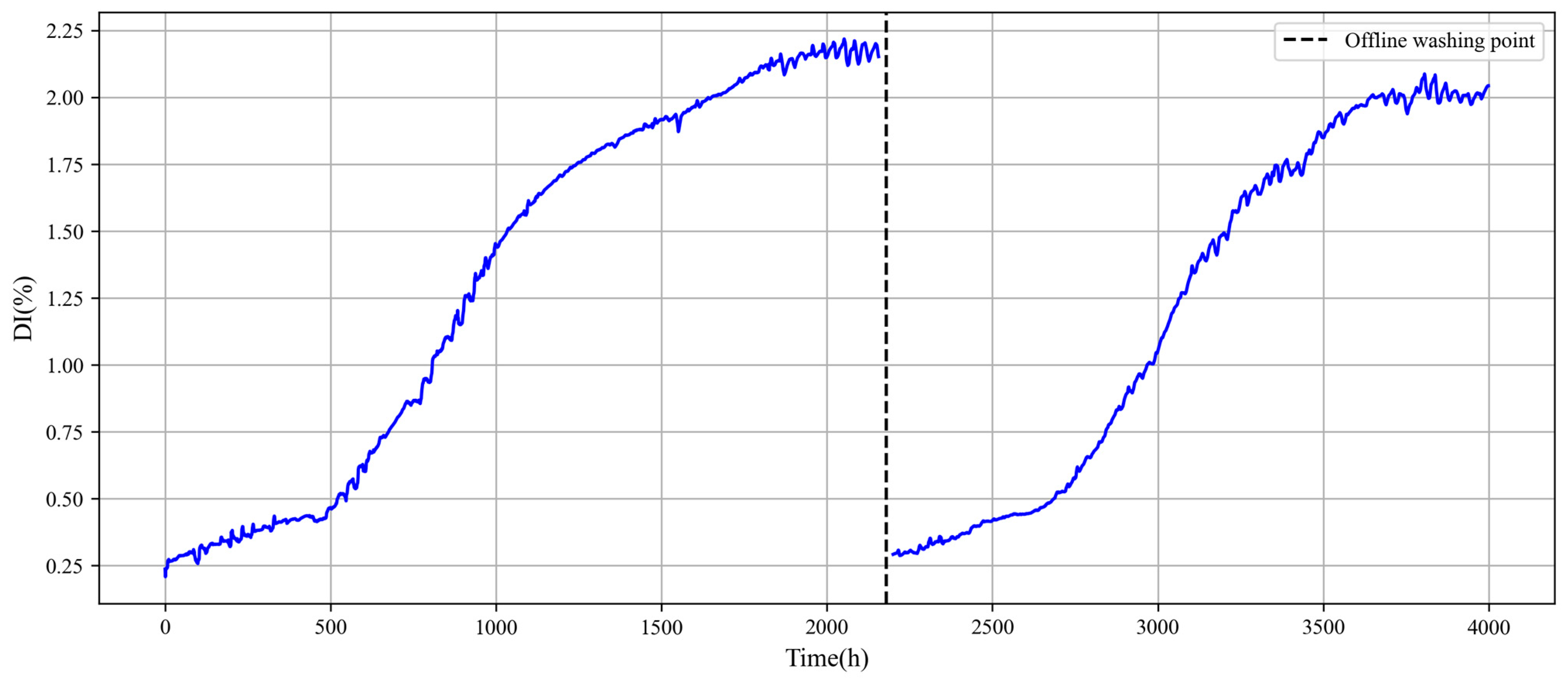
3.2. Performance Degradation Indicator Calculation

Compressor fouling is taken as an example to verify the proposed method. Assuming there is only compressor fouling and no other failures in the gas path components, fouling can be implemented by injecting the reduction in compressor efficiency into the mechanism model, thus simulating the accumulation of compressor fouling. The trend of compressor efficiency change over time can be referenced from the real degradation trend described in Ref. [20].

To better simulate the actual operating conditions, the real ambient temperature change was used as an input for the mechanism model to generate 4000 h of operation data. A comparison between the actual and predicted values of the exhaust temperature and compressor polytropic efficiency is shown in Figure 8. Polytropic efficiency is considered in this study to express the loss of the compressor aerodynamic performances; it is a more accurate term used to determine the degradation of the components than isentropic efficiency. Polytropic efficiency takes into account not only the start and the end of the compression and expansion processes but also the path of these processes [31]. Compressor polytropic efficiency [32] can be calculated using the following formula:

$${\eta }_c=\frac{T_1\left({\pi }^{\frac{\gamma -1}{\gamma }}-1\right)}{T_2-T_1}=\frac{{\pi }^{\frac{\gamma -1}{\gamma }}-1}{\theta -1}$$

(19)

where $\pi$ represents the pressure ratio of the compressor, $\gamma$ represents the specific heat ratio, and $\theta$ represents the temperature ratio at the inlet and outlet of the compressor.

In Figure 8, it can be observed that the variation in ambient temperature leads to significant fluctuations in both exhaust temperature and compressor polytropic efficiency. As the operating time increases, the exhaust temperature of the gas turbine shows an overall increasing trend. This is mainly due to the gradual accumulation of deposits on the compressor blades, resulting in a decline in compressor performance and a reduction in the output power of the gas turbine. To maintain the same output power, the control system increases the fuel mass flow rate. After washing, the exhaust temperature decreases, and compressor polytropic efficiency rises again.

Considering that compressor polytropic efficiency can better reflect the performance degradation of the compressor components, the residual of compressor polytropic efficiency is selected as the performance degradation indicator $\mathcal{D}\mathrm{I}$ of the compressor components. $\mathcal{D}\mathrm{I}$ is calculated for each moment according to Equation (12), and the results are shown in Figure 9. It can be observed that the growth of $\mathcal{D}\mathrm{I}$ in the second washing cycle is faster than that in the first washing cycle, but there is a certain similarity in the growth trend. Therefore, $\mathcal{D}\mathrm{I}$ of the first washing cycle can be used to train the prediction model, and the trend can be predicted based on the real-time calculation of $\mathcal{D}\mathrm{I}$ in the second washing cycle.

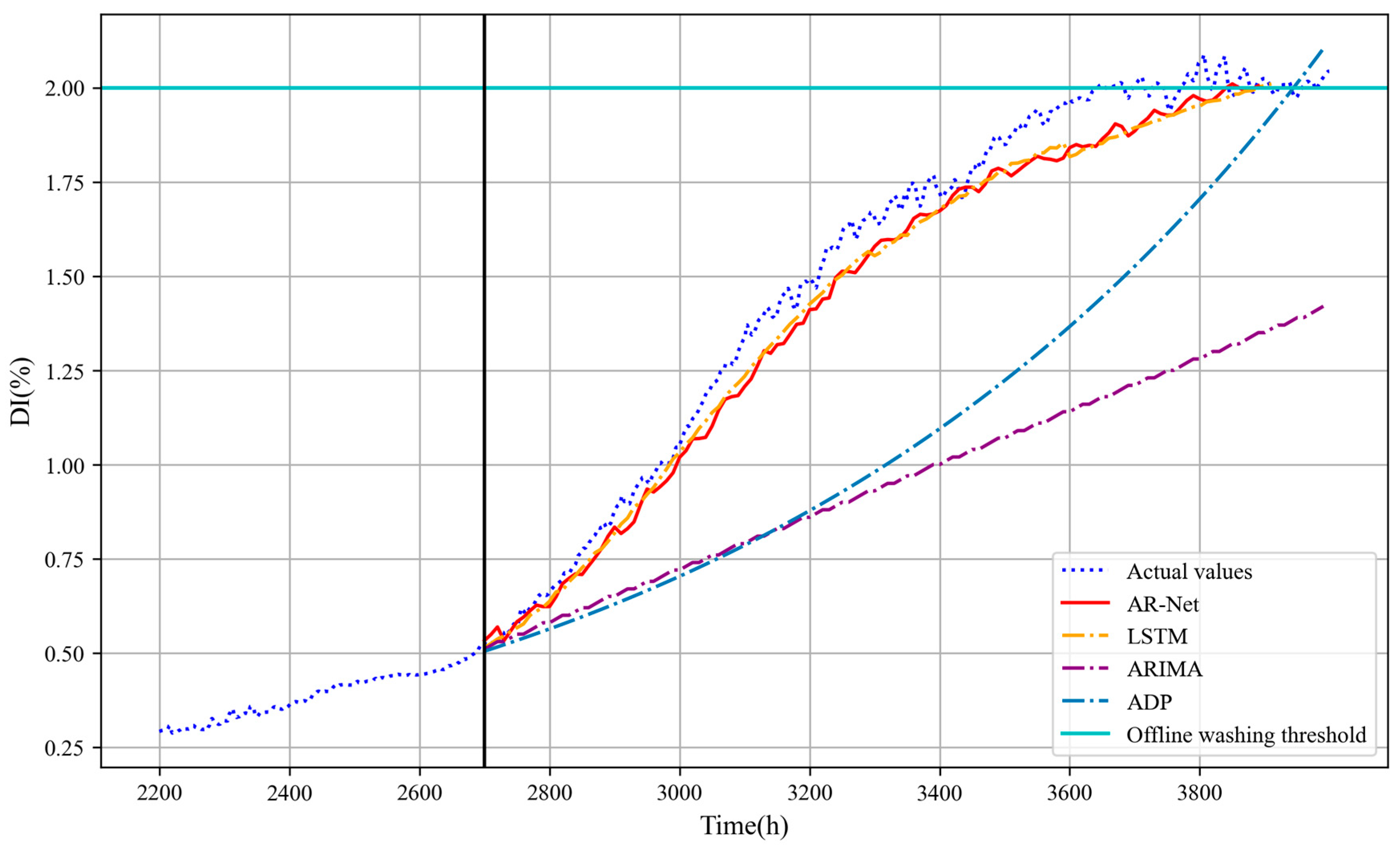
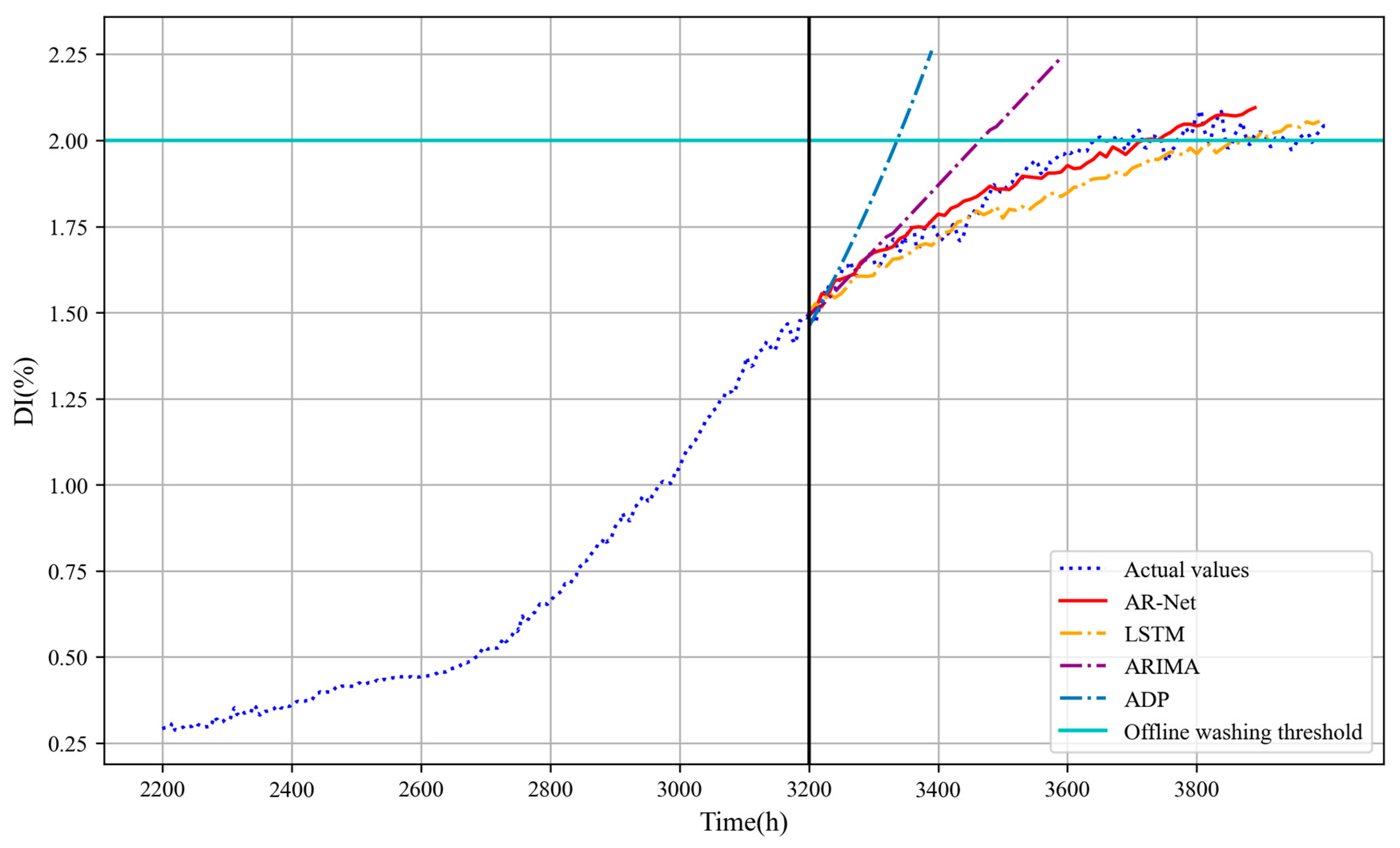
3.3. Prediction Model Validation and Comparison

In this study, the hyperparameters of the AR-Net prediction model were set as follows: the historical time step p was set to 500, the prediction step h was set to 300, and two hidden layers with sizes of 64 and 32 were set. Then, the piecewise linear model mentioned in Section 2.4 was used to smooth the $\mathcal{D}\mathrm{I}$ in the first washing cycle and used as the training set to train the network weights of the AR-Net model. The training results are shown in Figure 10, and the RMSE of the prediction model on the training set is 0.03, indicating that the prediction model can fit the $\mathcal{D}\mathrm{I}$ well in the first washing cycle.

Next, the proposed prediction model was used to predict the $\mathcal{D}\mathrm{I}$ in the second washing cycle. In order to compare the predictive performance of different models, three other models were selected as comparisons, including LSTM [20], ARIMA [18], and ADP [19].

Table 4. Hyperparameter settings for the models.

Model	Setting
AR-Net	Input steps: 500 Output steps: 300 First hidden layer size: 64 Second hidden layer size: 32
LSTM	Input steps: 500 Output steps: 300 First hidden layer size: 64 Second hidden layer size: 32
ARIMA	AR order: 500 Integrated order: 3 MA order: 500
ADP	The number of data points fitted: 500

lists the hyperparameter settings of each model.

Table 5. Comparison of prediction models.

	AR-Net		LSTM		ARIMA		ADP
Time (h)	RMSE	MAPE	RMSE	MAPE	RMSE	MAPE	RMSE	MAPE
500	0.08	5.10	0.08	4.80	0.58	33.42	0.47	29.24
1000	0.06	2.51	0.09	4.49	0.33	14.37	1.00	46.37

shows the predictive accuracy of the four models at different prediction times. Due to their failure to capture the trend of historical washing data, both ARIMA and ADP exhibit significant errors in forecasting both the final washing time and $\mathcal{D}\mathrm{I}$ changes during the prediction process, making them only suitable for short-term forecasting. LSTM and AR-Net both show good long-term predictive accuracy, with AR-Net exhibiting a significantly improved predictive performance over time and outperforming LSTM.

Figure 11 and Figure 12 show the predictive performance of the four models at different prediction times, assuming a threshold of 2 for $\mathcal{D}\mathrm{I}$. The black vertical line marks the beginning of the prediction results. It can be observed that although LSTM is capable of making predictions, it does not adjust in real time based on the trend of historical values, resulting in similar results for both predictions. On the other hand, AR-Net provides relatively accurate predictions for different operating times. When the operating time is 500 h, due to limited historical data, AR-Net can only make predictions based on the historical data from the previous washing cycle, resulting in some lag in the predictions. However, when the operating time reaches 1000 h, AR-Net accurately learns the faster upward trend and provides more precise predictions based on the latest $\mathcal{D}\mathrm{I}$. Therefore, AR-Net outperforms LSTM as a prediction model and can accurately identify the accelerating trend of engine performance degradation.

4. Conclusions

In order to optimize the maintenance cycle of gas turbines, this paper proposes a novel data-driven method for predicting the performance degradation of gas turbines. Based on an SVR performance model, the gas path performance parameters under healthy conditions can be obtained, and then the residual values $\mathcal{D}I$ between the predicted and actual values are calculated. Finally, the AR-Net prediction model is used to accurately predict $\mathcal{D}I$ for a future period of time, which is used to determine the maintenance time. By simulating the real fouling trend of the compressor and comparing it with the other three models, the correctness of the proposed method is verified. The results show the following:

• The predicted values of the SVR performance model and measured parameters can be used to calculate $\mathcal{D}I$. After smoothing with a piecewise linear model, the influence of environmental conditions and control factors is eliminated to some extent.
• The prediction model based on AR-Net can accurately predict the performance degradation of gas turbines over time and demonstrates the superiority of the proposed method compared to other models.
• In practical engineering applications, various degradation indicators, such as residual power output and residual exhaust temperature, can be used to comprehensively assess the performance degradation trend of a gas turbine and its components. This allows for better scheduling of turbine maintenance, thus optimizing operational costs and major overhaul time.

References

- Hanachi, H.; Liu, J.; Ding, P.; Kim, I.Y.; Mechefske, C.K. Predictive compressor wash optimization for economic operation of gas turbine. J. Eng. Gas Turbines Power. 2018, 140, 121006. [Google Scholar] [CrossRef]
- Kurz, R.; Brun, K. Degradation of gas turbine performance in natural gas service. J. Nat. Gas Sci. Eng. 2009, 1, 95–102. [Google Scholar] [CrossRef]
- Tahan, M.; Tsoutsanis, E.; Muhammad, M.; Karim, Z.A. Performance-based health monitoring, diagnostics and prognostics for condition-based maintenance of gas turbines: A review. Appl. Energy 2017, 198, 122–144. [Google Scholar] [CrossRef]
- Schneider, E.; Demircioglu Bussjaeger, S.; Franco, S.; Therkorn, D. Analysis of compressor on-line washing to optimize gas turbine power plant performance. J. Eng. Gas Turbines Power. 2010, 132, 062001. [Google Scholar] [CrossRef]
- Kurz, R.; Brun, K. Gas Turbine Tutorial-Maintenance and Operating Practices Effects on Degradation and Life. In Proceedings of the 36th Turbomachinery Symposium; Texas A&M University, Turbomachinery Laboratories: College Station, TX, USA, 2007; pp. 173–186. [Google Scholar]
- Hanachi, H.; Mechefske, C.; Liu, J.; Banerjee, A.; Chen, Y. Performance-based gas turbine health monitoring, diagnostics, and prognostics: A survey. IEEE Trans. Reliab. 2018, 67, 1340–1363. [Google Scholar] [CrossRef]
- Hanachi, H.; Liu, J.; Banerjee, A.; Chen, Y.; Koul, A. A Physics-Based Performance Indicator for Gas Turbine Engines Under Variable Operating Conditions. In Proceedings of the ASME Turbo Expo 2014: Turbine Technical Conference and Exposition, Düsseldorf, Germany, 16–20 June 2014. [Google Scholar]
- Blinstrub, J.; Li, Y.G.; Newby, M.; Zhou, Q.; Stigant, G.; Pilidis, P.; Hönen, H. Application of Gas Path Analysis to Compressor Diagnosis of an Industrial Gas Turbine Using Field Data. In Proceedings of the ASME Turbo Expo 2014: Turbine Technical Conference and Exposition, Düsseldorf, Germany, 16–20 June 2014. [Google Scholar]
- Lu, F.; Ju, H.; Huang, J. An improved extended Kalman filter with inequality constraints for gas turbine engine health monitoring. Aerosp. Sci. Technol. 2016, 58, 36–47. [Google Scholar] [CrossRef]
- Lu, F.; Gao, T.; Huang, J.; Qiu, X. Nonlinear Kalman filters for aircraft engine gas path health estimation with measurement uncertainty. Aerosp. Sci. Technol. 2018, 76, 126–140. [Google Scholar] [CrossRef]
- Rahmoune, M.B.; Hafaifa, A.; Kouzou, A.; Chen, X.; Chaibet, A. Gas turbine monitoring using neural network dynamic nonlinear autoregressive with external exogenous input modelling. Math. Comput. Simul. 2021, 179, 23–47. [Google Scholar] [CrossRef]
- Alam, M.M.; Bodruzzaman, M.; Zein-Sabatto, M.S. Online prognostics of aircraft turbine engine component’s remaining useful life (RUL). In Proceedings of the IEEE SOUTHEASTCON 2014, Lexington, KY, USA, 13–16 March 2014; pp. 1–6. [Google Scholar]
- Sun, L.; Liu, T.; Xie, Y.; Zhang, D.; Xia, X. Real-time power prediction approach for turbine using deep learning techniques. Energy 2021, 233, 121130. [Google Scholar] [CrossRef]
- Liu, Z.; Karimi, I.A. Gas turbine performance prediction via machine learning. Energy 2020, 192, 116627. [Google Scholar] [CrossRef]
- Palmé, T.; Liard, F.; Cameron, D. Hybrid Modeling of Heavy Duty Gas Turbines for On-Line Performance Monitoring. In Proceedings of the ASME Turbo Expo 2014: Turbine Technical Conference and Exposition, Düsseldorf, Germany, 16–20 June 2014. [Google Scholar]
- Li, Y.G.; Nilkitsaranont, P. Gas turbine performance prognostic for condition-based maintenance. Appl. Energy 2009, 86, 2152–2161. [Google Scholar] [CrossRef]
- Zhou, D.; Yu, Z.; Zhang, H.; Weng, S. A novel grey prognostic model based on Markov process and grey incidence analysis for energy conversion equipment degradation. Energy 2016, 109, 420–429. [Google Scholar] [CrossRef]
- Wang, W.; Li, S.; Wang, J.; Cui, B. Prediction on gas path performance degradation of gas turbine based on time series model. J. Eng. Therm. Energy Power 2016, 31, 50–55. [Google Scholar]
- Zagorowska, M.; Schulze Spüntrup, F.; Ditlefsen, A.-M.; Imsland, L.; Lunde, E.; Thornhill, N.F. Adaptive detection and prediction of performance degradation in off-shore turbomachinery. Appl. Energy 2020, 268, 114934. [Google Scholar] [CrossRef]
- Chen, J.; Tang, X.; Lu, J.; Zhang, H. A Compressor Off-Line Washing Schedule Optimization Method with a LSTM Deep Learning Model Predicting the Fouling Trend. J. Eng. Gas Turbines Power 2022, 144, 081005. [Google Scholar] [CrossRef]
- Jin, Y.; Liu, C.; Tian, X.; Huang, H.; Deng, G.; Guan, Y.; Jiang, D. A hybrid model of LSTM neural networks with a thermodynamic model for condition-based maintenance of compressor fouling. Meas. Sci. Technol. 2021, 32, 124007. [Google Scholar] [CrossRef]
- Triebe, O.; Laptev, N.P.; Rajagopal, R. AR-Net: A simple Auto-Regressive Neural Network for time-series. arXiv 2019, arXiv:1911.12436. [Google Scholar]
- Zhou, Z. Deep Learning Based Air Quality Prediction with Time Series Sensor Data; Arizona State University: Tempe, AZ, USA, 2023. [Google Scholar]
- Xiao, Z.; Huang, X.; Liu, J.; Li, C.; Tai, Y. A novel method based on time series ensemble model for hourly photovoltaic power prediction. Energy 2023, 276, 127542. [Google Scholar] [CrossRef]
- Shehzad, M.K.; Rose, L.; Azam, M.F.; Assaad, M. Real-Time Massive MIMO Channel Prediction: A Combination of Deep Learning and NeuralProphet. In Proceedings of the GLOBECOM 2022-2022 IEEE Global Communications Conference, Rio de Janeiro, Brazil, 4–8 December 2022; pp. 1423–1428. [Google Scholar]
- Wang, Z.; Gu, J.; Han, X.; Zhu, J.; Huang, Y. Reference Value Determination Based on Data Driven under Full Operating Conditions of Gas Turbine. Process Autom. Instrum. 2019, 40, 5–8+13. [Google Scholar]
- Awad, M.; Khanna, R.; Awad, M.; Khanna, R. Support vector regression. In Efficient Learning Machines: Theories, Concepts, and Applications for Engineers and System Designers; Springer: Singapore, 2015; pp. 67–80. [Google Scholar]
- Gao, F.; Kou, P.; Gao, L.; Guan, X. Boosting regression methods based on a geometric conversion approach: Using SVMs base learners. Neurocomputing 2013, 113, 67–87. [Google Scholar] [CrossRef]
- Taylor, S.J.; Letham, B. Forecasting at scale. Am. Stat. 2018, 72, 37–45. [Google Scholar] [CrossRef]
- Zhang, F.; Cheng, L.; Wu, M.; Xu, X.; Wang, P.; Liu, Z. Performance analysis of two-stage thermoelectric generator model based on Latin hypercube sampling. Energy Convers. Manag. 2020, 221, 113159. [Google Scholar] [CrossRef]
- Najjar, Y.S.; Alalul, O.F.; Abu-Shamleh, A. Degradation analysis of a heavy-duty gas turbine engine under full and part load conditions. Int. J. Energy Res. 2020, 44, 4529–4542. [Google Scholar] [CrossRef]
- Wang, T. 15—The gas and steam turbines and combined cycle in IGCC systems. In Integrated Gasification Combined Cycle (IGCC) Technologies; Wang, T., Stiegel, G., Eds.; Woodhead Publishing: Sawston, UK, 2017; pp. 497–640. [Google Scholar]