Abstract
Although they are primarily installed for specific applications, decentralised energy systems, storage systems, and controllable loads can provide flexibility. However, this varies over time. This study investigates the fundamentals of flexibility provision, including quantification, aggregation, simulation, and impact on energy systems and the power grid. We extended our methods by integrating adjustments to calculate the flexibility potential of heat pumps (HPs) and heat storage (HS) systems, as well as by incorporating variability and uncertainty. The simulations revealed the relevance of energy systems operation to flexibility, e.g., 2 K deviation in HS temperature increased theoretical coverage by 16 percentage points. The results also proved that aggregating multiple systems could obviously enhance their flexibility potential, e.g., six investigated battery storage (BS) systems could have covered up to 20 percentage points more external flexibility requests than any individual unit. The provision of flexibility by decentralised energy systems can lead to energy surpluses or deficits. Such imbalances could have been fully balanced in a system- and grid-oriented manner in 44% of BS simulations and in 32% of HP-HS ones. Overall, the findings highlight the importance of the system- and grid-oriented operation of decentralised energy systems, alongside local optimisation, for a future energy infrastructure.
1. Introduction
The transition towards a decarbonised energy supply means a higher penetration of renewable energy systems that entail volatile electricity generation, such as wind turbines and photovoltaic (PV) systems, as well as an increasing ratio of electrification in the heating, cooling, and transportation sectors [1,2]. Nevertheless, the power grid must ensure a reliable and stable energy supply at each point in time despite the fluctuating nature of power generation by volatile renewable energy systems. Therefore, the grid must enhance flexibility by extending the existing portfolio with decentralised flexibility sources, such as integrated energy systems, storage systems, the solutions of demand side management and response, as well as power-to-X-to-power technologies [3,4].
Efforts in pursuit of this objective can already be observed nowadays. Mlecnik et al. [5], for instance, investigated market development in seven European countries and found that the business solutions for providing flexibility from buildings had mostly been developed by the retail industry, energy facilities companies, and aggregators. Since the beginning of 2024, distribution grid operators in Germany have been allowed to temporarily reduce the energy consumption of decentralised energy systems with installed capacities over 4.2 kW in the case of potential grid overloads, as prescribed in §14a of the German Energy Industry Act [6]. Wanapinit et al. [7] estimated that the system-oriented operation (e.g., based on dynamic electricity prices) of battery storage (BS) systems installed in residential buildings could reduce electricity generation costs by 6% in comparison to operation for self-consumption optimisation. Adding the regional peak reduction as a secondary objective could also improve the loading of infrastructure in both the distribution and transmission grids.
As assumed in [8,9], the future power system may consist of multiple energy cells that can decide autonomously and within specified conditions about the operation of their local energy generators, storage systems, and loads. These energy cells could encompass, for example, residential, commercial and industrial buildings, quarters, city districts, and others, or even components or joined clusters of these. Different energy systems can be installed in energy cells, such as PV-BS systems, heat pumps (HPs), heat storage (HS) systems, combined heat and power (CHP) generators, charging stations for electric vehicles, systems for heating, ventilation and air conditioning, and other units. These systems have concrete primary applications, e.g., energy supply, optimisation of self-consumption, space heating, cooling, water heating, and further needs of energy cell occupants. However, they are technically able to provide flexibility inside and outside their energy cells by changing their initial or scheduled operation. Therefore, these technologies are referred to as flexibility providers in this paper.
In our previous study [10], we defined flexibility as the ability of energy cells and their components (e.g., power generators, storage systems, cross-sectoral integrated energy systems, and controllable loads) to deviate from optimally scheduled operations for balancing the fluctuations in energy generation and consumption without undermining the primary application of the components. As the overall capabilities of these energy systems are most of the time not fully exploited for their primary applications, we investigate the flexibility that remains after the operation of the energy systems has already been optimised to ensure their primary applications. For example, the operation of HP-HS systems must primarily be scheduled to provide the necessary amount of thermal energy for space and water heating. Then, the remaining capacity of this system to balance further deviations can be offered as flexibility inside or outside of the energy cells. The similar understanding of flexibility as the additional service was described and calculated using the example of BS systems by Tiemann et al. [11]. As the deviations can be presented by both power ramp ups and ramp downs, the flexibility can be distinguished as positive and negative. The need for positive flexibility requires an increase in energy generation or decrease in energy consumption, and the need for negative flexibility can be covered by the opposing actions [10].
The studies [3,12,13,14,15,16] have presented extensive literature reviews regarding energy flexibility, existing methods of flexibility quantification, as well as evaluation metrics. In our previous work [10], we also conducted a literature review concerning existing definitions of flexibility, methods for quantifying and assessing flexibility for general cases, various building types, and different energy technologies. Although the provision of flexibility belongs to the highly researched topics in recent decades, only a few studies have investigated the entire process of flexibility provision, including quantification, aggregation, the simulation of flexibility requests, the consideration of uncertainty, and other procedures. Danner et al. [17] proposed modelling the flexibility power of decentralised energy systems based on PV and load predictions and then aggregating the flexibility power boundaries of all investigated components in the pool. Afterwards, a flexibility request was disaggregated via the iterative assignment of flexibility portions to the most suitable components of the pool. Agbonaye et al. [18] developed and combined two methodologies: one for calculating the flexibility potential of decentralised energy systems and another for estimating flexibility needs from the congestion of transformers, ancillary services, and the dispatch of wind power systems. Furthermore, the authors assessed whether the calculated available flexibility potential coincided spatially and temporally with the estimated flexibility needs of the power grid. Früh et al. [19] investigated an entire process for the coordinated, vertical provision of flexibility from decentralised energy systems connected to distribution grids under consideration of grid constraints. First, they quantified and aggregated the flexibility potential of the energy systems from the bottom up. Second, they applied a top-down concept to disaggregate the flexibility requests that could be provided by a single energy system. To the best of the authors’ knowledge, no methodology has been developed for investigating the influence of flexibility provision on the further operation of decentralised energy systems and power grids if the flexibility is provided as the additional service, i.e., flexibility provision is a secondary (and not mandatory) application of the energy systems.
This study makes the following contributions to the energy flexibility research field: Its first contribution involves integrating specific calculation steps into the existing flexibility quantification method (developed in our previous work [10]) to quantify the flexibility of HP-HS technologies. Its second contribution is the development of an approach for integrating variability and uncertainty into the flexibility quantification method. And the third contribution involves analysing the impact of flexibility provision on the operation of energy cells and the power grid evaluated through the concept of flexibility return. To summarise, this study contributes to the research field by providing a comprehensive investigation, quantification, and evaluation of the entire process of flexibility provision based on the example of energy system simulations. To demonstrate the functionality of the developed methods, we calculated the theoretical flexibility potential of multiple decentralised energy systems belonging to diverse technologies and having different applications.
The current study is structured as follows: Section 2 contains the methodology, namely the fundamentals of the flexibility provision process. In Section 3, we present and discuss the results of the case studies to demonstrate the functioning of the proposed methodologies. Section 4 concludes the study and also presents an outlook for future research.
2. Methodology
In this Section, we present the theoretical basics for the entire process of providing flexibility by means of decentralised energy systems installed in energy cells for specific primary applications. This implies that flexibility provision is the secondary (non-mandatory) application of these energy cells components. The complete process of flexibility provision consists of the following procedures: (1) quantifying and aggregating the flexibility potential of different flexibility providers with consideration of local uncertainties, (2) providing the requested amount of flexibility and re-scheduling the operation of energy systems, and (3) calculating the impact of the flexibility provision for future operation of the local energy system and the power grid.
2.1. Quantifying the Flexibility Potential
In our previous work [10], we developed a method for quantifying the flexibility potential of decentralised energy systems that consists of three main calculation steps. These steps were explained in [10] for a general case as well as for a BS. As the heating sector has great potential for providing flexibility to the power grid, numerous studies have proposed frameworks for quantifying and evaluating the flexibility of electricity-based heating systems, e.g., [20,21,22]. In this study, we extend the existing method of our previous work [10] to quantify the flexibility potential of HP-HS systems. The technology-specific, as well as operational schedule specific steps, for quantifying the flexibility potential of these technologies are explained in the following.
Step 1: Schedule. The operation of HP-HS systems is scheduled to produce the necessary amount of thermal energy, e.g., in a cost-optimal way, in order to ensure comfortable room temperature as well as sufficient hot water volume for building occupants. The input data contain time series with heat demand, scheduled HP electrical power consumption , and energy amount stored in the HS according to the schedule . In addition to that, the technical information of the energy systems is also taken into account, such as the nominal power and coefficient of performance (COP) of the HP, as well as the nominal volume of the HS.
Step 2: Calculation of boundaries. In this step, we propose defining and calculating the boundary values. By boundary values we are referring to the ability of the HP-HS system to deviate from typical or scheduled operation in terms of power and energy for the purpose of flexibility provision without undermining its primary application, namely space and water heating. The boundary for power depends on the nominal electrical power of the HP compressor . Therefore, the lower and upper power boundaries are defined as follows:
The boundary for energy consists of the minimal and maximal amount of energy that must be stored in the HS at time t, so that the heating system can be operated as scheduled until the end of the planning time. Here, planning time refers to a time interval for which the operation of the HP-HS system is scheduled to cover the heat demand. As the flexibility potential is quantified based on whether the heating system can both provide flexibility and cover the heat demand from the given point in time until the end of the planning period, the duration of this period must be defined beforehand.
where is the scheduled energy amount stored in the HS at time t and is the usable capacity of the HS.
Similar to our flexibility quantification method, the studies summarised by Wagner et al. [23] also proposed integrating the operational boundaries, amongst other values, in order to mathematically represent the behaviour of energy systems for investigating their optimised operation and flexibility provision.
Step 3: Calculation of the flexibility power and duration. The maximal duration of the flexibility provision from the HP-HS is equal to the time period in which the new operating power of the HP (the operating power changed according to the flexibility power () lies within the estimated power boundaries. Additionally, the scheduled capacity of the HS, together with additional capacity for the flexibility provision, must be inside the energy boundaries during this time period. Therefore, the maximal duration of the flexibility provision is given by
The output of the flexibility quantification method consists of two universal dimensions: the flexibility power in kW and the maximal duration in hours for which this flexibility power can be provided alongside the scheduled operation. The universality of the output enables the application of different metrics to evaluate the flexibility of various energy systems, regardless of their technologies or primary purposes, as well as to compare and aggregate their flexibility values.
2.2. Aggregating the Flexibility Values of Different Technologies
The orchestration of multiple decentralised energy systems for the purpose of combined flexibility provision increases the extent of flexibility potential, i.e., the combination can offer more flexibility in comparison to any single unit within it. The aggregated flexibility potential contains higher flexibility power values for longer periods of time. Moreover, aggregation can smoothen the flexibility potential of multiple energy systems.
In [10], we proposed a method for aggregating the flexibility values of the different energy systems. The main goal of this method was to estimate an optimal combination of energy systems to provide the requested flexibility power for the longest time considering the technological and schedule-specific characteristics of the energy systems in the combination. The input data include the flexibility power and duration values of any number of flexibility providers, which are combined for the aggregated flexibility provision. These values are quantified independently for each flexibility provider in the combination using the flexibility quantification method described in the previous subsection.
The output of the flexibility aggregation method consists of aggregated flexibility power and duration, as well as flexibility power values that the components in the combination contributed to the aggregated flexibility. The optimal combination of flexibility values was determined on the condition that the aggregated flexibility power can be provided as long as possible. A detailed explanation of the method for aggregating flexibility values, together with the necessary equations, is provided in our previous study [10].
2.3. Consideration of Local Flexibility Needs
In the current study, we assume that the energy cells reserve their residual load beforehand and strive to follow it. However, the deviations from this residual load occur because of variability in local energy consumption, the volatility of energy generated by the local weather-dependent renewable energy systems, energy forecast uncertainty, the failure of energy systems, etc. We assume that local flexibility providers, such as BS, HP-HS, controllable loads, and others, should strive to balance these local deviations. Therefore, the deviation in the internal power and energy consumption of the energy cell can be understood as local flexibility needs.
In general, the local flexibility needs can be presented with power and energy values, as we described in [24]. We propose considering the local flexibility needs by addition/subtraction of their power and energy values from the power and energy boundaries of the flexibility providers estimated in Step 2 of the flexibility quantification method (see Section 2.1). Therefore, the definite amount of power and energy is reserved for the case that the energy cells must mitigate their internal unexpected fluctuations, i.e., local flexibility needs.
where , present the lower and upper power boundaries, respectively, and , the lower and upper energy boundaries with consideration of local flexibility needs. and are reserved for balancing the unexpected local fluctuations in power and energy within the energy cells.
As the consideration of the local flexibility needs reduces the distance between lower and upper boundaries, the flexibility potential is quantified within the narrower range of power and energy. Therefore, the integration of the local flexibility needs into the flexibility quantification will cause a decrease in the theoretical flexibility potential that can be offered outside the energy cells.
2.4. Flexibility Provision and Flexibility Return
The flexibility provision of decentralised energy systems may cause energy surpluses or deficits at later points in time. Therefore, the energy systems inside energy cells may not be capable of following their initially scheduled operations and satisfying the needs of the building occupants. In other words, the flexibility provision may bring about negative impacts on energy cells and the power grid, e.g., a lack of thermal energy for space heating in buildings or additional power consumption during times of power grid overload. In order to prevent or minimise these negative impacts on both the local energy system and the power grid, the energy provided as flexibility should theoretically be returned. For instance, after providing negative flexibility by increased power consumption, this additionally consumed energy should be fed back into the power grid and vice versa.
To assess possible strategies for energy return, we propose the following method. The flexibility provision changes the amount of energy stored in the flexibility providers in comparison to the scheduled operation, e.g., a lower water temperature in HS in the case of positive flexibility provision or a higher water temperature in HS in the case of negative flexibility provision. Therefore, the new values of energy stored in the flexibility provider at time point t can be estimated as follows:
The developed method for flexibility quantification ensures that the operation of the energy systems, together with the flexibility provision, does not undermine the technical and schedule-specific boundaries within the planning time period. For instance, the power and state of charge of the BS must stay within the lower and upper boundaries during the entire planning time period. However, after this time period, the energy amount might undermine the technical boundaries (e.g., nominal capacity of the BS systems) if the operation is not adjusted properly until a certain point in time. Therefore, we define the following:
and
where denotes the cumulative amount of energy missing at time t in the case of a positive flexibility provision and the cumulative amount of energy exceeding in the case of negative flexibility provision. We term this function the flexibility return curve, as it describes the amount of energy that was previously provided as flexibility and should theoretically be returned to or removed from the flexibility provider. Compensating for the energy surpluses or deficits caused by flexibility provision ensures that flexibility providers operate within their technical boundaries, energy cells retain their initially scheduled operations, and additional overloading of the power grid is avoided.
As long as and are equal to zero, the energy deficit or surplus created by the flexibility provision do not negatively impact the operation of flexibility providers. Therefore, the flexibility return is still not mandatory, but possible. If the values of and drop below or rise above zero, the prior flexibility provision starts to bring about an energy deficit or surplus, respectively.
Figure 1 displays the schematic understanding of the flexibility return curve for the example of . The top plot presents the amount of energy stored in a flexibility provider during the initially scheduled operation (grey curve) and after the positive flexibility provision (red dashed curve). The middle plot depicts the extent to which the amount of energy in the storage falls below the lower energy boundary caused by the flexibility provision. Moreover, the bottom plot shows the cumulative energy deficit, i.e., the flexibility return curve. According to this figure, all of the energy provided as flexibility should theoretically be returned to the flexibility provider by 18:45.
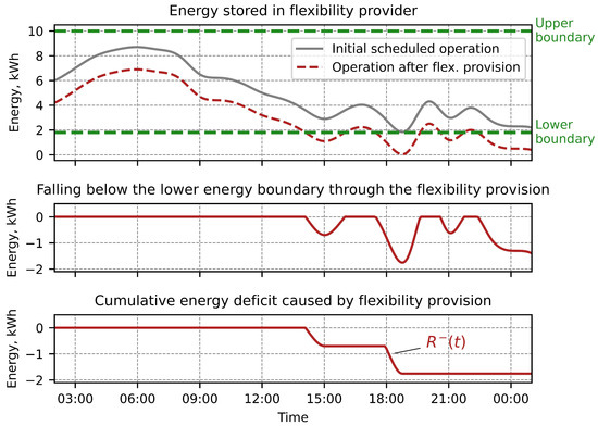
Figure 1.
Schematic presentation of the flexibility return curve for the example of .
To clarify, flexibility return does not refer to the obligatory physical reversal or withdrawal of the energy previously supplied as flexibility. This is an attempt to investigate and quantify the impact of flexibility provision on the further operation of decentralised energy systems, as well as to illuminate the necessary information for minimising negative impacts on the energy cells and the power grid.
3. Results and Discussion
The functional principle of all procedures within the flexibility provision, together with additional necessary calculations, are demonstrated in the example of HP-HS and PV-BS systems in residential buildings, as well as combinations of these technologies.
3.1. Data
This section describes the input data applied to quantify and aggregate the flexibility potential, as well as to simulate the flexibility provision and flexibility return.
3.1.1. Battery Storage Systems
The open access dataset EMSIG [25] contains the power measurements of eleven households in the DACH region (Germany, Austria, and Switzerland) recorded by home energy management systems from 1 October 2017 to 31 December 2020 with a time resolution of 15 min. The following measured values are included in the dataset: active power output of the PV system, load active power, fed in and drawn active power at the grid meter, charged and discharged active power of the BS, and the state of charge (SOC) of the BS.
All households have an identical BS system, Fenecon Pro 9–12, which features a nominal power of 9 kW and usable capacity of 12 kWh to maximise the self-consumption rate of local PV systems. As [25] does not provide the installed capacity of PV systems in the households, we derived these values from the highest measured PV power in the dataset. This value is well-suited for application in the modelling of PV system operation, as well as for making PV predictions, as presented in [26].
For our investigation, we selected six households from the EMSIG dataset in the period from 1 January 2019 to 31 December 2019. One of the main reasons for choosing these households was their negligibly small number of missing values in 2019. The key information about these households is summarised in Table 1. A more detailed description of the dataset can be found in [25].

Table 1.
Main information regarding the investigated households with the PV-BS systems in 2019 [25].
3.1.2. Heat Pumps and Thermal Storage Systems
The historical electrical power consumption of the HPs installed in 38 single-family houses (SFHs) in Northern Germany is collected in a publicly available dataset WPuQ [27]. For our investigations, we selected the measured data of six households with an available time resolution of 15 min. The main reasons for this were that the selected households do not have PV systems and their heat demands were mainly covered by the HP-HS systems, i.e., the HPs provided the required amount of thermal energy either without heating rods or the operation of the heating rods was negligibly low. Another relevant reason was that the measured time series of the selected households only had small amounts of missing values in 2019. Table 2 presents an overview of the annual energy consumption of the households, along with the annual and monthly energy consumption of their heat pumps. Further information about the dataset, as well as descriptions of data acquisition and its validation can be found in [27].
Table 2.
Main information regarding the investigated households with the HP-HS systems in 2019 [27].
3.1.3. Balancing Energy
We use the publicly available statistical data [28,29] and historical values of balancing energy for the year 2019 [30] to estimate the time and power that a single household can theoretically provide as flexibility to the power grid. The balancing energy is distinguished into (+) and (−). The “Balancing energy volume (+)” displays the necessary amount of energy (in MWh) to physically balance the energy deficit in the German transmission system within every 15 min. For instance, in the case of overestimation of the energy feed-in at a given time, the power grid requires more energy feed-in or less energy consumption. The opposite case is the energy surplus in the German transmission system presented by “Balancing energy volume (−)”. For example, in the case of underestimation at the given time interval, the power grid needs less energy feed-in or higher energy consumption [31].
The Federal Statistical Office of Germany counted 40.9 million households in 2019 [28]. According to [29], in 2019 approximately 21% of the households in Germany had at least one of the following flexibility technologies: PV, BS, HP, CHP, solar thermal systems, wood pellet heating systems, or electric vehicles. In accordance with this information, we assume for our simulations that 21% of German households could theoretically have provided energy flexibility to the power grid in 2019. Drawing on this assumption, together with the historical values of balancing energy, we calculated the flexibility power and energy requested from a single household, i.e., how much flexibility one household could theoretically have provided to cover the needs of balancing energy in 2019:
where presents the total balancing energy at the point in time t (from [30]), is the total amount of households, and is the share of the households utilising at least one flexibility technology. The total annual sum of the balancing energy, as well as the mean energy per household with at least one flexibility technology are presented in Table 3.
Table 3.
Main information regarding the balancing energy in 2019.
Figure 2 displays the calculated balancing power values per household in Germany per 15 min. In Figure 2 we do not recognise any pattern, such as the daily or seasonal dependency of the balancing power per household calculated using the historical measured values. The calculated balancing power per household, both (+) and (−), is in the range between −300 W and 300 W, apart from three outlier days in June 2019 when the values reached almost 900 W. In order to avoid possible confusion in understanding of the figure, we confirm that the balancing power (+) and balancing power (−) did not occur at the same time. Each time point contained either a single value of balancing power ((+) or (−)) or no value (no balancing energy was required). To demonstrate that, we inserted the bottom sub-plot in Figure 2, which displays the balancing power per household on a single day, 15 March 2019.
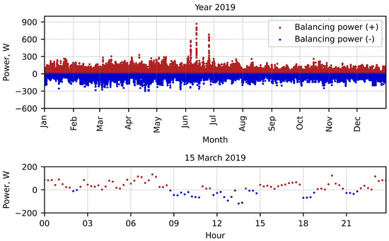
Figure 2.
Balancing power (+) and (−) per single household with at least one flexibility technology for the entire year of 2019 (top sub-plot), and for one day 15 March 2019 (bottom sub-plot). All values were calculated using the historical balancing energy for the year 2019 [30].
The historical balancing energy was chosen for the calculation of the balancing power per household because these values present the actual physical imbalance caused by the overestimation or underestimation of energy generation and consumption in the German power grid. As these amounts of energy were actually missed or exceeded, they had to be balanced by the available flexibility sources.
3.2. Flexibility Quantification
In our previous work [10] we demonstrated the developed method for quantifying flexibility in residential buildings with PV-BS systems. In this study, we applied the developed method to quantify the flexibility potential of HP-HS-systems in selected households that could also have provided it additionally to their operations in 2019.
The first step in the proposed flexibility quantification method prescribes scheduling the operation of the decentralised energy systems to cover the needs of building occupants. The original time-series with electrical power consumption of the HPs from [27] were used to derive the time-series with thermal power required for heat demand of the selected households (see Table 2). As the historical power measurements reflect the operational fluctuations of the heat pumps under real-world conditions, we assume that the derived heat demand also includes the corresponding kind of variability. This generated heat demand data were then applied to simulate the optimal operation of the HP-HS systems in the selected households using a generic MTRESS model [32,33].
These newly generated data contain time-series of the household heat demand, operating electrical power of the HPs, thermal power flow between HP and HS, as well as the amount of thermal energy stored in the HS systems at each point in time. The thermal energy stored in the HS was calculated using the difference between the flow and return temperatures. In the simulations of the scheduled operation (without flexibility provision), we defined that the nominal difference between the flow and return temperatures in the HS must not exceed 10 K, i.e., during the operation without flexibility provision the maximal nominal flow temperature was set to 40 °C and the return temperature to 30 °C.
In the second step of the method for quantifying flexibility, we defined and calculated the power and energy boundaries of the HP-HS systems. The lower power boundary of these systems is equal to zero and the upper power boundary to (set nominal power of the HP compressor). These power boundaries remain stable during the quantification of the flexibility potential of the HP-HS systems for the entire year of 2019. In comparison to that, the lower and upper energy boundaries should be calculated anew at all points in time for the planning period, the duration of which was set to six hours. However, this value is a free variable and can be changed according to the users of the flexibility quantification method.
In order to enable the simulation of the flexibility provision, we assumed that the HS was allowed to deviate by up to 5 K from its nominal temperature levels. In this case, the flow temperature in the HS could reach a maximal value of 45 °C during the provision of negative flexibility, and the return temperature was allowed to cool down to 25 °C during the provision of positive flexibility. The additional energy corresponding to the allowed temperature deviation in the HS was considered in the calculation of the energy boundaries, as well as in that of the amount of energy stored in the HS during and after the flexibility provision.
In the third step of the flexibility quantification method, we calculated the maximal duration for providing the flexibility power values. In order to investigate the entire flexibility potential of the HP-HS, we defined a range of positive and negative flexibility power values. The following range was defined ∈ [−4500, 4500] with a step of 100 W, where −4500 W was the maximal negative flexibility power and 4500 W the maximal positive flexibility power. We estimated the maximal duration of the flexibility provision for each flexibility power value in this range. Firstly, we calculated the new power values of the HP and new value of energy stored in the HS in case of deviation from the operation for the purpose of flexibility provision. Secondly, we determined that these new power and energy values lay between the lower and upper boundaries at each point in time over the subsequent six hours. Otherwise, the flexibility could not be provided. The flexibility potential was calculated for every 15 min time interval independently of each other.
To highlight, the primary objective of power and energy boundaries is to ensure the secure operation of energy systems, thereby meeting the needs of building occupants. As long as the flexibility potential is calculated within these boundaries, occupants will not experience any negative impact from flexibility provisions. In case of undermining the boundaries, the flexibility potential at that point in time is considered to be zero.
As the decentralised energy systems have different primary applications and can provide flexibility solely as an additional service, these systems feature a time-varying flexibility potential. In Figure 3, the daily variations in flexibility potential are presented for the example of the HP-HS system in “SFH-19” for two different times, 00:00 and 10:00, on 24 January 2019.
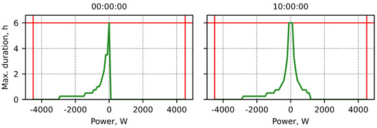
Figure 3.
Duration of different positive and negative flexibility power values in “SFH-19”, i.e., flexibility potential curves, at 00:00 and 10:00 on 24 January 2019.
The green curves in Figure 3 represent the flexibility potential for the entire flexibility power range at the given points in time. The vertical red lines correspond to the power boundaries, and the horizontal red line depicts the planning time of 6 h. At midnight on 24 January 2019, the HP-HS system in “SFH-19” could have almost solely provided the negative flexibility by additional increase of the HP electrical power. At 10:00 on the same day, this HP-HS system could have provided approximately similar amounts of positive and negative flexibility. The current operating mode of the HPs and energy amount stored in the HS systems have a strong influence on the flexibility potential.
In addition to daily variations, the HP-HS systems in the observed households also have seasonal variations in their flexibility potential. Figure 4 presents the maximal flexibility power that the HP-HS system in “SFH-19” could have provided as flexibility at each time point in 2019 for the maximal duration of 15 min.
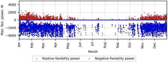
Figure 4.
Maximal flexibility power values that the HP-HS in “SFH-19” could have provided for the maximal duration of 15 min at each time point in 2019.
Each point in time in Figure 4 has two values indicated by two dots: the red dots correspond to the maximum positive flexibility potential, whereas the blue ones represent the maximum negative flexibility potential for the 15 min period. However, the flexibility potential also includes the intermediate power values between zero and the calculated maximum. For example, the calculated maximal power of the positive flexibility at 1000 W can be interpreted as the HP-HS system having theoretically reduced its power consumption by a value between 0 W and 1000 W for the purpose of positive flexibility provision.
The annual mean of all maximal positive flexibility power values during the heating period (from January to April and from October to December) was equal to 150 W for the maximal duration of 15 min. Over the same period of time, the annual mean of all maximal negative flexibility power values was much higher, at 1800 W. Thus, the HP-HS system in the selected household had much higher negative flexibility potential than positive. In other words, the flexibility potential could have been provided more frequently by switching on the HP.
Based on the flexibility potential curves for each point in time of the year 2019, we calculated the monthly mean flexibility potential curves for the selected points in time (00:00, 06:00, 12:00, and 18:00) independently from each other. The area under these monthly curves was then calculated using the trapezoidal rule (see Figure 5). The values of the area under the monthly mean flexibility potential curves demonstrate both the daily and seasonal variations in the flexibility potentials.
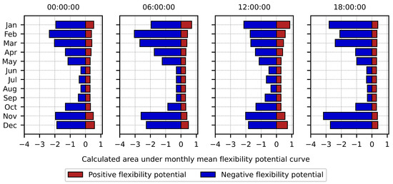
Figure 5.
Area under the monthly mean flexibility potential curves of the HP & HS in “SFH-19” calculated at the time points of 00:00, 06:00, 12:00, and 18:00 for 2019.
Similarly to Figure 4, the calculated area values under the mean flexibility potential curves demonstrate that the HP-HS system in “SFH-19” could have provided more negative flexibility than positive in 2019. Furthermore, the calculated flexibility potential in the colder months is higher than in warm ones, as the HP-HS systems were operated more frequently and intensively in the months with lower outside air temperatures to generate a sufficient amount of thermal energy for comfortable room temperature. As the investigated household had almost no heat demand in the warmer months, the HP-HS system was operated very rarely. In this regard, the flexibility potential during this time period was much lower. The HP-HS systems with another operational mode, such as for the provision of space and water heating as well as cooling, could have been operated during the entire year. Therefore, these systems could have had higher flexibility potential during the warm season.
3.3. Flexibility Aggregation
In this section, we demonstrate the flexibility aggregation method and describe the results of aggregating the flexibility potential values from two different technologies: BS and HP-HS. For this purpose, we selected a household “EMS-1” with a PV-BS system from [25] and a household “SFH-19” with an HP-HS system from [27]. These two households were selected for the flexibility aggregation case study, because based on data analysis we assumed that “EMS-1” did not have an electricity-based heating system, and that HP-HS system in “SFH-19” was operated primarily during the cold season. These two decentralised energy systems were therefore taken to belong to different technology categories, and to have different primary applications, technical characteristics, and operational schedules.
For the annual evaluation of the aggregated flexibility potential, we calculated the maximal aggregated flexibility power that the BS in “EMS-1” and HP-HS system in “SFH-19” could have provided together at each point in time for the maximal duration of 15 min in 2019. Figure 6 presents the mean weekly percentage contributions of the BS and the HP-HS system (top and bottom sub-plots) to the aggregated flexibility, as well as the maximal aggregated flexibility power that this combination could have provided at each point in time in 2019 for the maximal duration of 15 min (middle sub-plot).
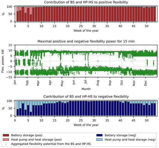
Figure 6.
Maximal aggregated flexibility power values that the HP and HS in “SFH-19” and BS systems in “EMS-1”could have provided together for the maximal duration of 15 min at each point in time in 2019.
Figure 6 shows that the BS system in “EMS-1” could have made much higher contributions to the aggregated flexibility potential, both positive and negative. The HP-HS system in “SFH-19” could have mostly influenced the aggregated negative flexibility in the cold season, when the heating system was operated much more intensively. Therefore, the aggregated negative flexibility potential during the cold season was higher than in the warm season. Almost all missing values of “EMS-1” occurred in the first, second, and fourth weeks of January, as well as the second week of February 2019. Therefore, the aggregated flexibility potential in these weeks was lower than in other cold months, and the HP-HS system has exhibited a higher contribution to the aggregated flexibility potential in these weeks. The mean annual contribution of the BS to the aggregated positive flexibility potential was 96.4% and to the aggregated negative flexibility potential it was 85.1%. The mean annual contribution of the HP-HS to the aggregated positive flexibility potential was 3.6% and to the aggregated negative flexibility potential it was 14.9%. The presented case study shows that the proposed method of flexibility aggregation can be applied to orchestrate different technologies for the joint flexibility provision.
One of the main goals of the flexibility aggregation is to increase flexibility power. The aggregated flexibility power from the combination of n flexibility providers should be higher than the flexibility power of each component participating in the flexibility provision. In addition, the flexibility aggregation method used in this study aims to identify the most optimal combination of available flexibility providers belonging to different technology types. Only the flexibility providers with available flexibility potential are included in the combination, and the participating flexibility providers are not obliged to contribute with equal power values to the aggregated flexibility. Therefore, each flexibility provider offers the flexibility potential that coincides with its schedule, as well as with the needs of the building occupants.
The flexibility aggregation case study revealed that the contribution of the selected HP-HS system to aggregated flexibility was relatively low. However, investigating and quantifying the flexibility potential of this technology remains highly relevant, as the number of installations is substantial and is expected to grow in the future. For example, in 2019, HPs were installed in 7% of German households, while BS systems were present in 2% [29]. By 2023, the share of households with HPs and BS systems had increased to 10.3% and 3.6%, respectively [34]. Furthermore, HP-HS systems can be incorporated to provide flexibility in cases when only this decentralised energy technology is available in the energy cells.
Nowadays, the majority of decentralised energy systems are operated to optimise the consumption of the buildings where these units are installed, e.g., the charging and discharging of the BS systems is scheduled to maximise the self-consumption of local PV systems. However, this kind of operation does not coincide with the requirements of the power grid and system balance, and it can even have negative impacts on them, such as overloading and increasing power grid and system costs [35,36]. Therefore, operation of decentralised systems in the future should consider both the local requirements as well as those of the power grid and system balance. Combining the high number of flexibility providers belonging to different technologies for joint flexibility provision can make a positive contribution to this goal.
3.4. Integration of PV Variability and Uncertainty into Flexibility Quantification
The next step in this investigation was to incorporate uncertainty into the flexibility quantification process. As we assume that local uncertainties should first be managed by available local flexibility providers, these uncertainties can also be interpreted as local needs for flexibility (see Section 2). In this case study, we demonstrated how to integrate these local flexibility needs into our developed flexibility quantification method using PV systems as an example. The local flexibility needs of PV systems are represented by unexpected power and energy fluctuations due to the variability and uncertainty inherent in their weather-dependent energy generation. In our previous study [24], we developed a framework for quantifying the power and energy fluctuations of any PV system using its historical power values. In this study, we integrated this framework into the method for quantifying the flexibility of energy cells.
First, we drew on the historical measured power values of PV systems from [25] to calculate the PV power ramps and build the cumulative empirical distributions of these. We assumed that 90% of these power fluctuations should first be balanced locally. By and , we denoted the 5% quantile and the 95% quantile, respectively. Thus, at each point in time the system should be able to balance the power fluctuation within the interval .
The results of this calculation are presented in Table 4, and can be interpreted as the power values of the local flexibility needs caused by the variability of the PV systems. Afterwards, were integrated into the calculation of lower and upper power boundaries of any flexibility provider using Equation (5). For example, 90% of the power ramps of the PV system in the household “EMS-5” lay in the range between −1.2 kW and 1.2 kW. Therefore, we assigned the value of 1.2 kW as the power value of the local flexibility needs caused by the PV system installed in this household.
Table 4.
Calculated power values of the local flexibility needs caused by PV variability.
We utilised global horizontal irradiance (GHI) data from Solcast [37] to predict the energy output of the PV systems using linear regression. This prediction contained a time series with the expected energy generation of these PV systems throughout 2019. Next, we calculated the absolute difference between the predicted and actually measured energy values at each time point during the year. We then averaged these absolute differences over the same points in time for the previous N days. In this study, we suggest that these average values represent the energy of local flexibility needs due to the uncertainty in PV systems. The relevant equation is presented below:
where and are the measured and predicted energy of the PV system at time t. To calculate for each point in time during the year, we used the absolute difference values between and at the same time as the previous five days, i.e., . For example, the energy value for local flexibility needs at 10:00 AM on 6 February 2019 was calculated by averaging the absolute difference values from the same time over the previous five days, specifically from 1 February 2019 to 5 February 2019. In this case, we considered the short-term weather trends and local site characteristics, but avoided consideration of long-term weather impacts over different seasons.
For demonstration purposes, Figure 7 displays the energy values of the local flexibility needs caused by the prediction uncertainty of the PV system in “EMS-1” in 2019. Each orange dot displays the corresponding energy of the local flexibility needs at the given point in time, which was calculated by averaging the absolute difference values between prediction and measurement at the same time for the previous five days. These values were integrated into the flexibility quantification method by subtracting them from the upper energy boundary and adding them to the lower one at each point in time, as described in Section 2.3. As is shown in Figure 7, the energy values exhibit a strong seasonal dependency. For example, during winter, when PV power generation is lower, the energy values for flexibility needs were expected to be much lower compared to those in summer.
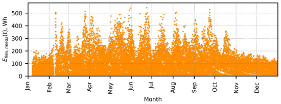
Figure 7.
Energy values of the local flexibility needs caused by the prediction uncertainty of the local PV system in “EMS-1”.
The inclusion of the power and energy fluctuations of PV systems in calculating the flexibility boundaries can be seen as the local flexibility provider setting aside a specific amount of power and energy to handle unexpected changes in local energy generation and consumption. On the one hand, considering local flexibility needs reduce the interval between the lower and upper boundaries, this in turn decreases the amount of theoretical flexibility potential available to meet external flexibility requests. On the other, it can keep the energy cell (e.g., city district) within its planned residual load, thereby avoiding additional costs and preventing potential overload of the local power grid. This operation of energy cells can be viewed as the system- and grid-oriented operation, which is essential for the future energy infrastructure.
3.5. Flexibility Provision
In the next phase of our research, we simulated how the investigated energy systems could respond to flexibility requests from external entities, such as public utility companies or distribution grid operators. We derived these requests from the balancing power per household outlined in Section 3.1.3. Specifically, we treated this balancing power as a flexibility requested from an individual household, where it deviates slightly from regular operation. At each point in time, we simulated whether the investigated BS and HP-HS systems could have met the corresponding flexibility request, i.e., balancing power per household at this point in time, without exceeding their power and energy boundaries during the planning period. For each simulation, the ability to provide balancing power was evaluated independently of other time points. This means that we assumed that the energy systems were operated according to their schedules before the flexibility requests were made.
We evaluated the simulation results using a metric called theoretical coverage. This metric quantifies the percentage of time points during which the analysed energy system could reliably provide balancing power as a flexibility for a maximum duration of 15 min, without exceeding its power and energy boundaries. Table 5 presents the annual theoretical coverage values of the BS systems with and without considering PV variability and uncertainty. The columns with household labels contain the theoretical coverage values of the single BS unit belonging to that household. The column “all” contains the theoretical coverage in the case of combining six BS systems to provide sixfold balancing power per household.
Table 5.
Theoretical coverage of the balancing energy by private households with PV-BS systems with and without consideration of the variability of PV systems.
As can be seen in Table 5, the individual BS systems (without consideration of local flexibility needs) could theoretically have covered approximately 60% of the balancing power values. The portions of positive and negative flexibility needs that can be covered by the BS systems are also approximately equal to each other.
As anticipated, considering the uncertainties in flexibility quantification reduced the overall external flexibility potential. Table 5 shows that setting aside a portion of power and energy to address potential local fluctuations in PV output led to a decrease in the average theoretical coverage values. The BS systems with consideration of the PV variability and uncertainty could have met about 15 percentage points less potential external flexibility requests in comparison to the BS systems without that consideration.
Aggregating six BS systems to provide the sixfold flexibility indeed enhanced their theoretical coverage. Specifically, this combination could have met almost 62% of the balancing power values when local flexibility needs were considered, and 83% when they were not. However, this aggregation could still not have covered the full range of requested balancing power values, despite the combined power of the six BS systems being significantly greater than the total balancing power required. The primary reason for this was the timing mismatch between the available flexibility potential of the BS systems and the requested balancing power. The timing mismatch means that the energy systems cannot provide flexibility at the times of the flexibility requests without undermining their primary applications. We assumed that the investigated BS systems were optimised to maximise the self-consumption of PV power, which did not always align with the external flexibility needs based on historical balancing energy.
The same simulation and evaluation were repeated for the HP-HS systems. The theoretical coverage of these was investigated for three levels of temperature deviations in the HS systems, and the results are presented in Table 6. The theoretical coverage values of the individual HP-HS units are presented in the columns with household labels, and the theoretical coverage of six HP-HS systems in the column “all”. The common operation of the HP-HS systems (without flexibility provision) was simulated under the condition that the flow temperatures could not exceed 40 °C and the return temperatures could not fall under 30 °C. For the simulation of the flexibility provision (especially in the calculations of thermal energy stored in HS as well as in that of the energy boundaries), we assumed that the flow and return temperatures were allowed to deviate from their nominal values by up to 5 K. For example, in the case of 2 K deviation, the HS systems were allowed to increase their flow temperatures to 42 °C—while increasing the losses of the HS—and decrease their return temperatures until 28 °C—while reducing the efficiency of the HP—for the purpose of flexibility provision.
Table 6.
Theoretical coverage of balancing energy by the private households with heat pumps together with thermal storage systems.
Allowing the HS systems to deviate from the nominal flow and return temperatures by up to 2 K led to a notable increase in the average theoretical coverage, improving it by approximately 16 percentage points compared to operations that did not allow deviation. Nevertheless, additional increases in the allowed deviation did not result in further improvements in the theoretical coverage values. The results from all three HP-HS simulations (with deviations by 0 K, 2 K, and 5 K) show that the investigated HP-HS systems were more effective at covering negative balancing power compared to positive balancing power. However, increasing the allowed temperature deviation had a stronger effect on improving the theoretical coverage for positive balancing power.
A central finding of the flexibility provision simulations was a significant increase in the flexibility that could have been provided by the combination of six BS systems or six HP-HS ones in comparison to single units. In other words, six investigated BS and HP-HS systems could have theoretically met more external flexibility requests derived from the balancing energy in comparison to the single units. Moreover, the results of the flexibility simulations confirmed that the operation of decentralised energy systems has a relevant influence on flexibility potential.
The aim of using the historical balancing energy values was to integrate the external requirements into the flexibility provision simulations. The results of the simulations confirmed once again that decentralised energy systems should be operated with consideration of both the local requirements and those of the power grid and system balance. Aggregating the flexibility of a large number of different energy systems can support this intention.
3.6. Flexibility Return
We investigated the influence of flexibility provision on the following operation of energy cells and the power grid with the help of the term flexibility return (see Section 2.4). For this purpose, we defined the external flexibility requests with longer durations and simulated the flexibility provision for these. For the definition of a flexibility request, we first selected the highest absolute value of balancing power per day and time of its occurrence. Then, we determined the time frame for flexibility provision such that all balancing power values in this interval had the same sign as the balancing power value at . This time frame was limited to two hours and and was at most one hour. We repeated this procedure for all days of the observed year of 2019.
First, we applied the flexibility quantification method to confirm that the investigated decentralised energy systems could have provided the required flexibility without undermining their power and energy boundaries over the next 6 h. If this condition was met, we then simulated the flexibility provision and corresponding deviation of these energy systems from the initial operation. Finally, we calculated the flexibility energy return curves as described in Section 2.4.
The operation of the energy systems in the following 24 h after flexibility provision was taken into account in the calculation of flexibility energy return curve. In this way, we intended to quantify the potential impacts on energy systems and households caused by deviation from their scheduled operation for the purpose of flexibility provision. For instance, because of the positive flexibility provision and resulting energy deficit in the BS system, the household load could not have been covered by the BS as initially planned. In addition, we also integrated the requirements of the surrounding energy system or power grid into the flexibility return quantification. In the worst case, the flexibility provision at a current point in time could lead to an additional system requirement in the future, such that the flexibility provider would not actually cover the need for flexibility but rather postpone it until later. For example, providing positive flexibility at a given point in time could cause higher energy consumption from the power grid later. In order to quantify the potential influence of flexibility provision on the power grid, we extended quantification of the flexibility return by inserting the balancing power per household into the calculations. For the flexibility return, we considered the balancing power values with a sign opposite that of the flexibility power provided. In this way, we attempted to quantify the possible negative effects on the power grid, as well as to make the entire process of flexibility provision more grid- and system-oriented. To summarise, the resulting flexibility return time series was created using both the time series with the operation of the decentralised energy systems and that with the balancing power per household in the following 24 h after the flexibility provision.
For the purpose of better understanding, we demonstrate the simulation results of the flexibility provision and return on the example of the BS system in “EMS-1” on 31 January 2019–1 February 2019. The historical operation of this BS system in the observed period of time can be derived from the scheduled SOC curve represented by the solid grey curve in Figure 8. The green dashed line indicates the minimum SOC value below which the BS cannot be discharged. According to the simulation, the BS received a request to provide 306.7 Wh of positive flexibility from 15:15 until 17:15. As the BS could have provided this required flexibility and kept its scheduled operation in the subsequent 6 h (according to the flexibility quantification method), we simulated the flexibility provision. However, the latter could have caused the energy deficit in the BS system in the following 24 h after the flexibility request, i.e., the SOC fell below its minimal value at 06:00 on 1 February 2019 (see the red dashed curve in Figure 8). Therefore, the energy deficit should theoretically be balanced until this point in time. Otherwise, the BS would not have sufficient energy to cover the household load, which would in turn consume more energy from the power grid.
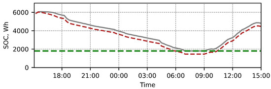
Figure 8.
SOC values of BS in “EMS-1” in the case of scheduled operation (grey curve) and flexibility provision (dashed red curve) on 31 January 2019–1 February 2019.
We calculated two energy curves, one being a cumulative energy deficit in the BS system in the 24 h following positive flexibility provision, and another being a cumulative available negative balancing energy per household in the following 24 h. Both curves are displayed in Figure 9.
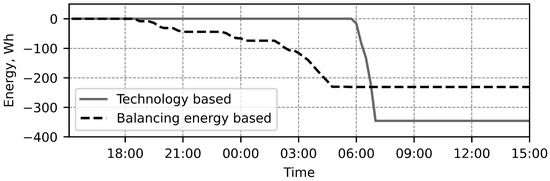
Figure 9.
Cumulative energy deficit of the BS in “EMS-1” caused by the positive flexibility provision (solid grey curve) and cumulative available negative balancing energy per household (dashed black curve) on 31 January 2019–1 February 2019.
Figure 9 shows that within the observed time period, the available negative balancing energy per household occurred before the critical time point at 06:00. Therefore, the energy deficit could theoretically have been balanced by providing this negative balancing power. Based on these two energy curves, we calculated the power values of the possible flexibility return considering both the operation of BS and the need for balancing power in the following 24 h. The power curve of the flexibility provision by the BS system in “EMS-1”, as well as the power curve of the flexibility return, are presented in the top subplot in Figure 10. The power curve of the flexibility provision (red solid curve) corresponds to the positive flexibility request that was defined as described at the beginning of this Section. The power curve of the flexibility return (blue dashed curve) was calculated considering the operating power of the BS and the available negative balancing power per household. As can be seen, the flexibility return curve includes power values with a sign opposite the power values of the flexibility provision.
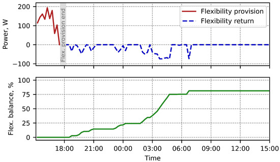
Figure 10.
Top subplot: power values of the positive flexibility (red curve) provided by the BS in “EMS-1” and those of the flexibility return (blue curve). Bottom subplot: flexibility balance (green curve) of the BS in “EMS-1” on 31 January 2019–1 February 2019.
In order to assess the simulation results, we calculated the flexibility balance, which is the percentage of energy provided as flexibility that can be returned within the next 24 h by providing the balancing power with a sign opposite the provided flexibility power values. The flexibility balance is a metric for evaluating the extent to which the flexibility provision can be managed in as a much system- and grid-oriented manner as possible. Within the demonstrated time period, 81.3% of the energy provided as positive flexibility by the BS in “EMS-1” could have been balanced by providing the negative balancing power, as is shown in the bottom subplot in Figure 10.
As is shown in Figure 10, the energy deficit caused by the positive flexibility provision on 31 January 2019 could not have been fully balanced by providing the negative balancing energy. However, as the flexibility return was managed by providing the negative balancing energy per household, this flexibility return means that this BS system provided flexibility to the power grid again.
We repeated these simulations for the entire year of 2019 and all the investigated energy systems. Then, we calculated the annual flexibility balance values of all investigated energy systems (see Table 7).
Table 7.
Calculated mean annual flexibility balance values for all households in 2019.
During the observed year, 55% of the flexibility provided by the BS in “EMS-1” could have been returned by supplying the balancing power with a sign opposite the power values of the flexibility provision. The HP-HS systems in “SFH-8” and “SFH-9”, which are supposed to be operated year-round, have higher flexibility balance values compared to other HP-HS systems that are only supposed to be operated during the cold season (October to April). The flexibility balance values indicate that in 44% of the BS cases and 32% of the HP-HS ones (mean values averaged over all investigated energy systems) the operation of the decentralised energy systems and power grid was not adversely affected by the flexibility provision. This was achieved by balancing the resulting energy surplus or deficit via the flexibility return approach.
The flexibility balance of 100% signifies situations in which the energy deficits or surpluses caused by flexibility provision were fully balanced in a system- and grid-oriented manner, meaning that the flexibility provision at that point in time did not create new flexibility requests in the power grid. However, operation of the decentralised energy systems and power grid in 2019 did not always feature optimal conditions for balancing the energy deficits or surpluses within the 24 h following flexibility provision. Despite this, any remaining portion of the energy surpluses or deficits could theoretically be balanced at a later time through coordinated efforts between the power grid and decentralised energy systems if necessary or required.
4. Conclusions and Outlook
4.1. Conclusions
In this study, we investigated the fundamentals of the flexibility provision process: the quantification of potential, aggregation, consideration of uncertainty, the simulation of provision and evaluation of impacts using the example of the multiple PV-BS and HP-HS systems in residential buildings in 2019. The results of the study demonstrate that the developed flexibility quantification method can be applied for calculating the time-varying flexibility potential of diverse decentralised energy systems that belong to different technologies, and have various primary applications, and therefore different operational schedules. The output of our flexibility quantification method consists of universal values, such as flexibility power and the duration of providing the given power. Thus, numerous evaluation metrics can be applied to assess and compare the flexibility of decentralised energy systems without technological restrictions.
The time-varying flexibility potential of energy systems is significantly influenced by their modes of operation, the amount of energy stored in the BS and HS systems at a given time and their planned operation following flexibility provision. For instance, the impact of the operational mode on the flexibility potential was clearly evident in the investigated HP-HS systems. If the operational temperature of the HS systems was allowed to deviate by up to 2 K from the set levels to provide flexibility, the HP-HS systems under investigation could have met approximately 16 percentage points more flexibility requests.
The flexibility aggregation method was demonstrated on the basis of the example of one BS and one HP-HS system. The selected HP-HS system could have contributed much less to the aggregated flexibility by comparison to the BS system. Nevertheless, the combination of the high number of energy systems belonging to different technologies for the purpose of joint flexibility provision can offer the following benefits: first, aggregation increases the flexibility power values, and second, it contributes to the system- and grid-oriented operation of decentralised energy systems.
The operating power of the investigated BS systems often remained below their nominal capacity, indicating a potential for greater flexibility, both in increasing and decreasing power output. In contrast, the investigated HPs typically operated either near their nominal power or were switched off entirely. This inflexible operating mode reduced the flexibility potential of the HP-HS systems. Incorporating the building envelope into flexibility quantification could theoretically enhance the flexibility potential of HP-HS systems by increasing overall storage capacity. However, this approach requires additional input data and more complex calculations, making it more challenging to quantify the flexibility of HP-HS systems compared to BS ones. Despite these challenges, HP-HS systems can still offer valuable flexibility in energy cells where other flexibility providers are unavailable, making their inclusion in future flexibility portfolios essential. Each unit in such a portfolio can contribute to maintaining system balance and ensuring stable operation of the power grid.
The next step was the integration of variability and uncertainty into the flexibility quantification. For this purpose, the power and energy fluctuations caused by variability and uncertainty were proposed to be considered in the second calculation step when quantifying the power and energy boundary values of the flexibility providers. A definite amount of power and energy could therefore be reserved for cases where local flexibility providers would have to mitigate these unexpected fluctuations. The integration of variability and uncertainty was demonstrated with the example of PV-BS systems. On the one hand, the BS systems could have power and energy reserved to mitigate the internal power and energy fluctuations of own PV systems at each point in time. On the other, BS systems taking into account the variability and uncertainty could have covered 15 percentage-points less potential external flexibility requests than those without this consideration.
For the simulation of flexibility provision, the external flexibility requests per household were derived from historical balancing energy data in Germany for 2019. Each investigated BS (excluding PV fluctuations) could theoretically have met approximately 60% of the external flexibility requests, whereas each HP-HS (with a 2 K temperature deviation) could have met approximately 50% of these requests. Although the nominal power and capacity of the investigated BS and HP-HS systems exceeded the balancing power per household, a single unit was still insufficient to fully satisfy these requests on its own. The primary reason for this was that the locally optimised operation of these energy systems did not temporally align with the flexibility requests derived from balancing energy. However, the aggregation of energy systems led to an increase in the theoretical coverage of flexibility requests. A combination of six BS systems could theoretically cover up to 20 percentage points more flexibility requests, and a combination of six HP-HS units could cover up to 14 percentage points more flexibility requests, compared to individual ones.
Decentralised energy systems can undergo energy deficits or surpluses after providing positive or negative flexibility, respectively. To address this, we quantified the amount of energy that is either exceeding or missing in these energy systems at each point in time over the subsequent 24 h period following the flexibility provision. In addition, we analysed historical balancing energy data to identify appropriate time periods within the next 24 h when the energy provided as flexibility could be theoretically fed into or consumed from the power grid without causing additional overload. By combining this information, we developed a flexibility return energy curve. The simulation results indicated that nearly half of the flexibility provided by the BS systems and one-third of that provided by the HP-HS systems could theoretically be returned without adversely affecting the power grid. In these cases, the external flexibility needs were sustainably met, rather than merely postponed.
Decentralised power generators, storage systems, and controllable loads have the potential to provide flexibility in addition to their primary applications, both within the energy cells in which they are installed as well as outside to support system balance and power grid requirements. We assume that providing flexibility within the energy cells reduces their external flexibility needs, and may therefore contribute to the more system- and grid-oriented operation of the energy cells. However, even with a large number of these decentralised energy systems in operation, they will not be sufficient to meet all future flexibility needs. We strongly assume that they will constitute just one potential source of flexibility in the future energy infrastructure. The future portfolio of flexibility sources will also include energy systems in industrial and commercial properties, hydrogen storage systems, fuel cells-based power generators, district heating networks, and other technologies. In principle, flexibility should be developed and provided from all available sources across all voltage levels of the power grid.
4.2. Outlook
Future research can adapt the developed method to quantify and aggregate the flexibility potential of other technologies, including electric vehicles, CHP systems, district heating networks, and various controllable loads. Furthermore, the proposed methodology could be applied to data of decentralised energy systems in other countries with varying climate conditions and energy consumption profiles. In such cases, the flexibility potential would likely exhibit different values and distinct daily and seasonal patterns. Additionally, future studies could explore the influence of other variability and uncertainty sources on the flexibility potential, such as load prediction uncertainty, the risk of energy system failures, and variations in occupant behaviour. Moreover, this study can serve as a fundamental basis for future studies regarding the economic feasibility, business models and flexibility markets for providing flexibility as an additional service of decentralised energy systems.
Developing, integrating, and supporting the flexibility provision of decentralised energy systems require a combination of technical solutions, business models, regulatory frameworks, and social acceptance. Technical recommendations include, among other things, the widespread roll-out of smart meters and smart energy management systems, as well as the standardisation of communication interfaces across all stakeholders. The smart energy management systems have to ensure optimal operation of energy systems and avoid possible negative impacts of flexibility provision on efficiency, service life, and other key performance characteristics. Therefore, these systems are responsible for overall system efficiency while maintaining optimal performance.
It is further recommended that end users, including private households and residential districts, be encouraged to optimise the operation of local energy systems according to their specific needs while also providing flexibility to support system balance and meet power grid requirements. To promote such system- and grid-oriented operation, the integration of dynamic electricity tariffs and/or variable network charges should be considered. Accordingly, energy supply companies are encouraged to offer dynamic electricity tariffs to all categories of end users. Another key recommendation concerns distribution grid operators that have to develop and integrate a low-voltage control centre enabling grid transparency, real-time monitoring, load management, automated control, as well as compliance with regulatory frameworks.
Neighbouring buildings equipped with decentralised energy systems might be recommended to establish an energy-sharing community to aggregate their flexibility potential values. This approach enables internal energy and flexibility management as well as support of system balance and provision of aggregated flexibility to the power grid. The necessary regulatory framework should ensure that the provision of flexibility for system and grid purposes aligns, or at least does not hinder or conflict with, the self-optimisation of decentralised energy systems for end user needs. To enable the effective flexibility provision of decentralised energy systems, collaboration among all stakeholders is essential, including manufacturers and operators of energy technologies, smart meters, energy management systems, energy supply companies, power grid operators, communities, legislators, and relevant governmental organisations.
Author Contributions
Conceptualization and methodology, N.M. and S.S.; software and simulation, N.M.; validation, N.M.; writing—original draft preparation, N.M.; writing—review and editing, S.S., B.H. and K.v.M.; visualization, N.M.; supervision, S.S.; project administration, S.S. and K.v.M.; funding acquisition, B.H. and K.v.M. All authors have read and agreed to the published version of the manuscript.
Funding
This research received no external funding.
Data Availability Statement
The original data applied in the study are available in the publicly accessible repositories [25,27,30].
Acknowledgments
The authors thank Cody Hancock for his support in the simulation of thermal energy supply in single-family houses.
Conflicts of Interest
The authors declare no conflicts of interest.
Abbreviations
The following abbreviations are used in this manuscript:
| BS | Battery storage |
| HP | Heat pump |
| HS | Heat storage |
| PV | Photovoltaic |
References
- International Renewable Energy Agency (IRENA). World Energy Transitions Outlook 2023: 1.5 °C Pathway. 2023. Available online: www.irena.org/Publications/2023/Jun/World-Energy-Transitions-Outlook-2023 (accessed on 3 July 2024).
- Agora Energiewende und Forschungsstelle für Energiewirtschaft e.V. Haushaltsnahe Flexibilitäten Nutzen. Wie Elektrofahrzeuge, Wärmepumpen und Co. die Stromkosten für alle Senken Können. 2023. Available online: www.agora-energiewende.de/publikationen/haushaltsnahe-flexibilitaeten-nutzen (accessed on 3 July 2024).
- Lund, P.D.; Lindgren, J.; Mikkola, J.; Salpakari, J. Review of energy system flexibility measures to enable high levels of variable renewable electricity. Renew. Sustain. Energy Rev. 2015, 45, 785–807. [Google Scholar] [CrossRef]
- Babatunde, O.; Munda, J.; Hamam, Y. Power system flexibility: A review. Energy Rep. 2020, 6, 101–106. [Google Scholar] [CrossRef]
- Mlecnik, E.; Parker, J.; Ma, Z.; Corchero, C.; Knotzer, A.; Pernetti, R. Policy challenges for the development of energy flexibility services. Energy Policy 2020, 137, 111147. [Google Scholar] [CrossRef]
- Federal Ministry for Economic Affairs and Climate Action. Energy Industry Act (EnWG). 2024. Available online: https://www.gesetze-im-internet.de/enwg_2005/BJNR197010005.html (accessed on 6 May 2024).
- Wanapinit, N.; Offermann, N.; Thelen, C.; Kost, C.; Rehtanz, C. Operative Benefits of Residential Battery Storage for Decarbonizing Energy Systems: A German Case Study. Energies 2024, 17, 2376. [Google Scholar] [CrossRef]
- Ardone, A.; Arens, M.; Ahrens, M.; Apel, K.; Baatar, M.; Bauknecht, D.; Bekk, A.; Binder, J. 1.5 °C. Energiewende Zellulär—Partizipativ—Vielfältig Umgesetzt; C/sells Selbstverlag: Stuttgart, Germany, 2020. [Google Scholar]
- Lehmann, N.; Huber, J.; Kießling, A. Flexibility in the context of a cellular system model. In Proceedings of the 2019 16th International Conference on the European Energy Market (EEM), Ljubljana, Slovenia, 18–20 September 2019. [Google Scholar] [CrossRef]
- Maitanova, N.; Schlüters, S.; Hanke, B.; von Maydell, K. An analytical method for quantifying the flexibility potential of decentralised energy systems. Appl. Energy 2024, 364, 123150. [Google Scholar] [CrossRef]
- Tiemann, P.H.; Nebel-Wenner, M.; Holly, S.; Frost, E.; Martinez, A.J.; Nieße, A. Operational flexibility for multi-purpose usage of pooled battery storage systems. Energ. Inform. 2022, 5, 13. [Google Scholar] [CrossRef]
- Alizadeh, M.; Parsa Moghaddam, M.; Amjady, N.; Siano, P.; Sheikh-El-Eslami, M. Flexibility in future power systems with high renewable penetration: A review. Renew. Sustain. Energy Rev. 2016, 57, 1186–1193. [Google Scholar] [CrossRef]
- Lopes, R.A.; Chambel, A.; Neves, J.; Aelenei, D.; Martins, J. A Literature Review of Methodologies Used to Assess the Energy Flexibility of Buildings. Energy Procedia 2016, 91, 1053–1058. [Google Scholar] [CrossRef]
- Li, H.; Wang, Z.; Hong, T.; Piette, M.A. Energy flexibility of residential buildings: A systematic review of characterization and quantification methods and applications. Adv. Appl. Energy 2021, 3, 100054. [Google Scholar] [CrossRef]
- del Granado, P.C.; Rajasekharan, J.; Pandiyan, S.V.; Tomasgard, A.; Kara, G.; Farahmand, H.; Jaehnert, S. Flexibility Characterization, Aggregation, and Market Design Trends with a High Share of Renewables: A Review. Curr. Sustain. Energy Rep. 2023, 10, 12–21. [Google Scholar] [CrossRef]
- Li, H.; Johra, H.; de Andrade Pereira, F.; Hong, T.; Le Dréau, J.; Maturo, A.; Wei, M.; Liu, Y.; Saberi-Derakhtenjani, A.; Nagy, Z.; et al. Data-driven key performance indicators and datasets for building energy flexibility: A review and perspectives. Appl. Energy 2023, 343, 121217. [Google Scholar] [CrossRef]
- Danner, D.; Seidemann, J.; Lechl, M.; de Meer, H. Flexibility disaggregation under forecast conditions. In Proceedings of the Twelfth ACM International Conference on Future Energy Systems, e-Energy’21, New York, NY, USA, 28 June–2 July 2021. [Google Scholar]
- Agbonaye, O.; Keatley, P.; Huang, Y.; Ademulegun, O.O.; Hewitt, N. Mapping demand flexibility: A spatio-temporal assessment of flexibility needs, opportunities and response potential. Appl. Energy 2021, 295, 117015. [Google Scholar] [CrossRef]
- Früh, H.; Müller, S.; Contreras, D.; Rudion, K.; von Haken, A.; Surmann, B. Coordinated Vertical Provision of Flexibility From Distribution Systems. IEEE Trans. Power Syst. 2023, 38, 1834–1844. [Google Scholar] [CrossRef]
- Masy, G.; Georges, E.; Verhelst, C.; Lemort, V.; André, P. Smart grid energy flexible buildings through the use of heat pumps and building thermal mass as energy storage in the Belgian context. Sci. Technol. Built Environ. 2015, 21, 800–811. [Google Scholar] [CrossRef]
- Fischer, D.; Wolf, T.; Triebel, M.A. Flexibility of heat pump pools: The use of SG-Ready from an aggregator’s perspective. In Proceedings of the 12th IEA Heat Pump Conference, Rotterdam, The Netherlands, 15–18 May 2017; Volume 15, pp. 1–11. [Google Scholar]
- Xu, X.; Lyu, Q.; Qadrdan, M.; Wu, J. Quantification of Flexibility of a District Heating System for the Power Grid. IEEE Trans. Sustain. Energy 2020, 11, 2617–2630. [Google Scholar] [CrossRef]
- Wagner, L.P.; Reinpold, L.M.; Kilthau, M.; Fay, A. A systematic review of modeling approaches for flexible energy resources. Renew. Sustain. Energy Rev. 2023, 184, 113541. [Google Scholar] [CrossRef]
- Maitanova, N.; Schlüters, S.; Hanke, B.; von Maydell, K.; Agert, C. Quantifying power and energy fluctuations of photovoltaic systems. Energy Sci. Eng. 2022, 10, 4496–4511. [Google Scholar] [CrossRef]
- Musikhina, D.; Seidemann, J.; Feilmeier, S. Energy Data Recorded by Decentralized Household Energy Management Systems (EMS). 2021. Available online: https://openenergy-platform.org/dataedit/view/demand/emsig_energy_data_by_ems (accessed on 5 February 2024).
- Maitanova, N.; Telle, J.S.; Hanke, B.; Grottke, M.; Schmidt, T.; Maydell, K.V.; Agert, C. A Machine Learning Approach to Low-Cost Photovoltaic Power Prediction Based on Publicly Available Weather Reports. Energies 2020, 13, 735. [Google Scholar] [CrossRef]
- Schlemminger, M.; Ohrdes, T.; Schneider, E.; Knoop, M. Dataset on electrical single-family house and heat pump load profiles in Germany. Sci. Data 2022, 9, 558. [Google Scholar] [CrossRef] [PubMed]
- Table Zeitvergleich Haushalte from Article Haushalte nach Haushaltsgrößen im Zeitvergleich. 2019. Available online: https://www.destatis.de/DE/Themen/Gesellschaft-Umwelt/Bevoelkerung/Haushalte-Familien/Tabellen/1-3-privathaushalte-neuer-zeitvergleich.html (accessed on 29 May 2024).
- KfW-Energiewendebarometer. Haushalte Möchten Mehr Erneuerbare Energien Nutzen—Durchbruch der Elektromobilität bis 2030 Erwartet; Technical Report; KfW Bankengruppe: Frankfurt am Main, Germany, 2019; Available online: https://www.kfw.de/ (accessed on 29 May 2024).
- SMARD Market Data. Available online: https://www.smard.de/en/downloadcenter/download-market-data/ (accessed on 31 May 2024).
- SMARD.de User Guide. 2021. Available online: https://www.smard.de/en/user-guide (accessed on 31 May 2024).
- Schönfeldt, P.; Schmeling, L.; Wehkamp, S. Model Template for Residential Energy Supply Systems (MTRESS), Version v2.2.0.; Zenodo: Genève, Switzerland, 2023. [CrossRef]
- Schönfeldt, P.; Grimm, A.; Neupane, B.; Torio, H.; Duran, P.; Klement, P.; Hanke, B.; Maydell, K.V.; Agert, C. Simultaneous optimization of temperature and energy in linear energy system models. In Proceedings of the 2022 Open Source Modelling and Simulation of Energy Systems (OSMSES), Freiburg, Germany, 7–9 September 2022; pp. 1–6. [Google Scholar] [CrossRef]
- KfW-Energiewendebarometer. Energiewende im Spannungsfeld Zwischen Handlungsbedarfen und Finanziellen Möglichkeiten; Technical Report; KfW Bankengruppe: Frankfurt am Main, Germany, 2023; Available online: https://www.kfw.de/ (accessed on 5 June 2024).
- Flexibilisierung des Energiesystems. VDE Study. VDE Verband der Elektrotechnik Elektronik Informationstechnik e.V., Offenbach am Main, Germany. 2023. Available online: https://www.vde.com/de/etg/arbeitsgebiete/v2/flexibilisierung-des-energiesystems (accessed on 2 July 2024).
- Eicke, A.; Hirth, L.; Mühlenpfordt, J. Mehrwert Dezentraler Flexibilität. Oder: Was Kostet die Verschleppte Flexibilisierung von Wärmepumpen, Elektroautos und Heimspeichern? Kurzstudie; Brief study; Neon Neue Energieökonomik GmbH: Berlin, Germany, 2024; Available online: https://neon.energy/mehrwert-flex/ (accessed on 4 July 2024).
- SOLCAST Data API. Available online: https://solcast.com/ (accessed on 11 April 2024).
Disclaimer/Publisher’s Note: The statements, opinions and data contained in all publications are solely those of the individual author(s) and contributor(s) and not of MDPI and/or the editor(s). MDPI and/or the editor(s) disclaim responsibility for any injury to people or property resulting from any ideas, methods, instructions or products referred to in the content. |
© 2024 by the authors. Licensee MDPI, Basel, Switzerland. This article is an open access article distributed under the terms and conditions of the Creative Commons Attribution (CC BY) license (https://creativecommons.org/licenses/by/4.0/).