A Numerical Investigation of Flow Characteristics in a Cryogenic Perforated Plate Flowmeter for Vertical Pipe Applications

Abstract

To address the research gap regarding the flow characteristics of cryogenic perforated plate flowmeters in vertical pipes and to enhance measurement reliability in challenging environments, this study investigates the flow characteristics of liquid hydrogen in a vertical pipe using a perforated plate flowmeter. Numerical simulations are performed based on an extended derivation of performance parameter formulas in the vertical direction. Various inlet Reynolds numbers, plate thicknesses, and equivalent diameter ratios are analyzed to assess their effects on key performance parameters, including the discharge coefficient, pressure loss coefficient, and stable region. The results indicate that the influence of flow direction on the performance parameters decreases with increasing Reynolds number. Downward flow is associated with smaller discharge coefficients, lower pressure loss coefficients, and reduced upper limits of Reynolds numbers in the stable region. Furthermore, the effects of gravity become more pronounced at larger thicknesses and greater equivalent diameter ratios.

1. Introduction

Flow measurement at cryogenic temperatures is vital in industries that require precise handling of cryogenic fluids, such as the liquefied natural gas (LNG) sector [1,2], hydrogen fuel processing [3,4], and aerospace applications [5,6,7]. Due to the instability of the cryogenic fluids’ phase, accurately measuring their flow rates presents significant challenges. However, precision in these measurements is critical not only for operational efficiency but also to ensure safety and minimize fluid loss. Perforated plate flowmeters have gained extensive attention in these applications due to their durability, simple structure, ability to balance flow fields, reduce vortex formation, and suitability for cryogenic environments [8,9,10,11].

In cryogenic conditions, fluid properties such as viscosity and density vary significantly, which may intensify the effects of gravitational forces and buoyancy, especially in vertical flow configurations. Vertical flow in perforated plate flowmeters, as opposed to horizontal flow, involves complex interactions between gravitational effects and pressure gradients, creating unique flow characteristics that affect the performance of flowmeters. In addition, for differential pressure devices, cavitation is a common phenomenon [12,13,14]. Due to the lower gas–liquid density ratio and thermal conductivity of cryogenic fluids compared to fluids at room temperatures, as well as the increased sensitivity of certain physical properties to temperature changes, the thermal effects during cavitation cannot be overlooked [15,16]. Furthermore, gravitational forces may also have a significant influence on the formation and collapse of cavitation bubbles under cryogenic conditions.

The current studies have extensively investigated the effect of structures of perforated plate flowmeters. Zhao et al. [17] conducted experiments using water and identified the equivalent diameter ratio as the primary factor influencing the pressure loss characteristics of perforated plates. Huang et al. [18] investigated the effects of geometric shape and upstream disturbances on the discharge coefficient of perforated plates with water. Mehmood et al. [19] focused on the effect of surface geometry parameters of perforated plates on the length of downstream development through numerical simulations. It indicated that increasing the number of holes can improve the static pressure recovery length of the downstream pipeline. Some scholars have carried out research on the application of perforated plate flowmeters to cryogenic fluids. Liu et al. [20] conducted theoretical and experimental research and found that the perforated plates have a larger upper limit in Re number for the cryogenic fluids than the room-temperature fluids. Jin et al. [21] simulated the flow of liquid hydrogen and concluded that perforated plates with the distribution of holes matching the turbulent velocity distribution in the circular tube are more suitable for liquid hydrogen measurement. Using liquid nitrogen, Zhao et al. [22] simulated and attributed the performance improvement of double-stage perforated plates over single-stage perforated plates to the “thickness effect”. Peng et al. [23] built an experimental setup for liquid nitrogen and, combined with numerical simulations, found that increasing the thickness can improve the pressure recovery rate, thereby reducing pressure loss.

It can be observed that the studies mainly focus on flow in horizontal pipes. However, these findings are often inadequate for applications of cryogenic fluids in vertical setups, as they fail to account for the unique forces and flow behaviors encountered under these conditions. Gravitational effects can alter the distribution of velocity and pressure, potentially introducing measurement errors if not properly considered [24]. However, existing research predominantly investigates horizontal flow setups, with a limited focus on the performance of cryogenic flowmeters in vertical applications. Thus, examining the flow characteristics of cryogenic fluids in vertical pipes remains an important gap in research.

Building upon existing studies, this research explores the flow characteristics of cryogenic perforated plate flowmeters in vertical pipes, focusing on how changes in inlet Reynolds number, plate thickness, and equivalent diameter ratio affect performance. By analyzing the effects of these factors under cryogenic conditions, this study fills a gap in the research on the flow characteristics of cryogenic fluids in vertical pipes and provides a theoretical basis for the optimization of flowmeters in vertical configurations.

The findings of this study will provide valuable insights for optimizing the design and operational parameters of cryogenic flowmeters in vertical pipe applications, especially in industries dealing with low-temperature fluids. The results offer theoretical support for the design of efficient flowmeters suitable for cryogenic fluids, improving the reliability, accuracy, and efficiency of flow measurement systems. This is critical for developing high-precision cryogenic flow meters and has significant implications for the design and operation of flow measurement systems in relevant industries.

2. Working Principle and Key Performance Parameters

Figure 1 is the working principle diagram of the perforated plate. It can be seen that when the fluid flows through the perforated plate from upstream, the pressure first drops and then recovers due to the throttling effect.

According to the principles of fluid mechanics, there is a quantitative relationship between the pressure difference formed across the orifice plate and the fluid flow rate. For an incompressible fluid, assuming the pipe has an inner diameter of D and a cross-sectional area of A, and the smallest contracted flow area is A₀, the Bernoulli equation and continuity equation can be applied to the upstream Section 2 and the smallest contracted Section 0. Thus, the following can be derived:

$${\displaystyle \frac{p_2}{\rho }}+c_2{\displaystyle \frac{u_2^2}{2}}+g{y}_2={\displaystyle \frac{p_0}{\rho }}+c_0{\displaystyle \frac{u_0^2}{2}}+g{y}_0+\xi {\displaystyle \frac{u_0^2}{2}}$$

(1)

$$A{u}_2=A_0{u}_0$$

(2)

where p_i, u_i, and y_i represent the average pressure, average flow velocity, and longitudinal position at section i, respectively; c₂ and c₀ refers to the kinetic energy correction factor at Sections 2 and 0; ρ is the density of fluid; g is the gravitational acceleration; and ξ is the total resistance coefficient of the orifice plate; A₀ is the smallest contracted flow area, calculated using the contraction coefficient μ and the equivalent diameter ratio β:

$$\mu ={\displaystyle \frac{A_0}{A_h}}$$

(3)

$$\beta =\sqrt{{\displaystyle \frac{A_h}{A}}}$$

(4)

where A_h represents the total area of all holes on the plate.

By solving Equations (1)–(4) simultaneously, the following can be obtained:

$$u_0={\displaystyle \frac{1}{\sqrt{c_0+\xi -c_1{\mu }^2{\beta }^4}}}\sqrt{{\displaystyle \frac{2\mathsf{\Delta }{p}_0}{\rho }}+2g\mathsf{\Delta }{y}_0}$$

(5)

$$\mathsf{\Delta }{p}_0=p_2-p_0$$

(6)

$$\mathsf{\Delta }{y}_0=y_2-y_0$$

(7)

where $\mathsf{\Delta }{p}_0$ is the maximum pressure difference caused by the throttling of the perforated plate, which occurs at the point of the minimum flow cross-section, labeled as Section 0. Since the position of this minimum contracted section varies depending on the flow speed and the characteristics of the perforated plate, it is not a fixed value. Therefore, a pressure coefficient $\psi$ is introduced to relate $\mathsf{\Delta }{p}_0$ to the actual measured pressure difference$\mathsf{\Delta }p$. Furthermore, based on Figure 1, the pressure variation between Sections 2 and 0 can be approximated as linear, leading to the following conclusion:

$$\psi ={\displaystyle \frac{\mathsf{\Delta }{p}_0}{\mathsf{\Delta }p}}\approx {\displaystyle \frac{\mathsf{\Delta }{y}_0}{\mathsf{\Delta }y}}$$

(8)

where $\mathsf{\Delta }y$ is the distance between the actual pressure taking positions before and after the perforated plate (positions 2 and 3 in Figure 1).

Based on the Formulas (3)–(5) and (8), the actual measured flow rate of the fluid is derived as follows:

$$\begin{array}{c}{q}_v=A_0{u}_0={\displaystyle \frac{\mu A_h}{\sqrt{c_0+\xi -c_1{\mu }^2{\beta }^4}}}\sqrt{{\displaystyle \frac{2\mathsf{\Delta }{p}_0}{\rho }}+2g\mathsf{\Delta }{y}_0}\\ \approx {\displaystyle \frac{\mu {\beta }^{2}A}{\sqrt{c_0+\xi -c_1{\mu }^2{\beta }^4}}}\sqrt{{\displaystyle \frac{2\psi \mathsf{\Delta }p}{\rho }}+2g\psi \mathsf{\Delta }y}\\ ={\displaystyle \frac{\mu {\beta }^{2}A\sqrt{\psi }}{\sqrt{c_0+\xi -c_1{\mu }^2{\beta }^4}}}\sqrt{{\displaystyle \frac{2\mathsf{\Delta }p}{\rho }}+2g\mathsf{\Delta }y}\#\end{array}$$

(9)

Assuming an ideal situation where the fluid velocity distribution in the pipeline is uniform and there is no energy loss, the total area of the orifices in the perforated plate is the minimum contracted area of the fluid. Additionally, the measured pressure difference is exactly the maximum differential pressure caused by the throttling, with the kinetic energy correction factor c₂, c₀ equal to 1, ξ = 1, μ = 1, $\psi$= 1. The theoretical flow rate in this case is

$$q_v^{\mathrm{\prime }}={\displaystyle \frac{{\beta }^{2}A}{\sqrt{1-{\beta }^4}}}\sqrt{{\displaystyle \frac{2\mathsf{\Delta }p}{\rho }}+2g\mathsf{\Delta }y}$$

(10)

Introducing the discharge coefficient C, which characterizes the ratio between the actual flow rate and the theoretical flow rate, the formula is given as

$$C={\displaystyle \frac{4q_v\sqrt{1-{\beta }^4}}{\pi D^2{\beta }^4}}\sqrt{{\displaystyle \frac{\rho }{2\mathsf{\Delta }p+2\rho g\mathsf{\Delta }y}}}$$

(11)

During the simulation, after obtaining the pressure difference across the orifice plate at the corresponding pressure tapping points, the C can be determined using Equation (11). The larger and more stable the C, the better the performance of the flowmeter.

For orifice flowmeters, another important parameter is the permanent pressure loss after the fluid passes through the orifice plate, which reflects the energy consumption of the fluid. The smaller the permanent pressure loss, the better the performance of the flowmeter. In practical applications, a dimensionless pressure loss coefficient ζ is often used to evaluate the pressure loss characteristics of the flowmeter. The relevant calculation formula is as follows.

$$\zeta ={\displaystyle \frac{\mathsf{\Delta }\omega }{0.5\rho u^2}}$$

(12)

where $\mathsf{\Delta }\omega$ is the permanent pressure loss, which is the static pressure difference measured between 1D upstream and 6D downstream (pressure taking positions 1 and 4 in Figure 1) of the orifice plate, and u represents the average flow velocity at the inlet.

3. Numerical Model and Validation

3.1. Physical Model

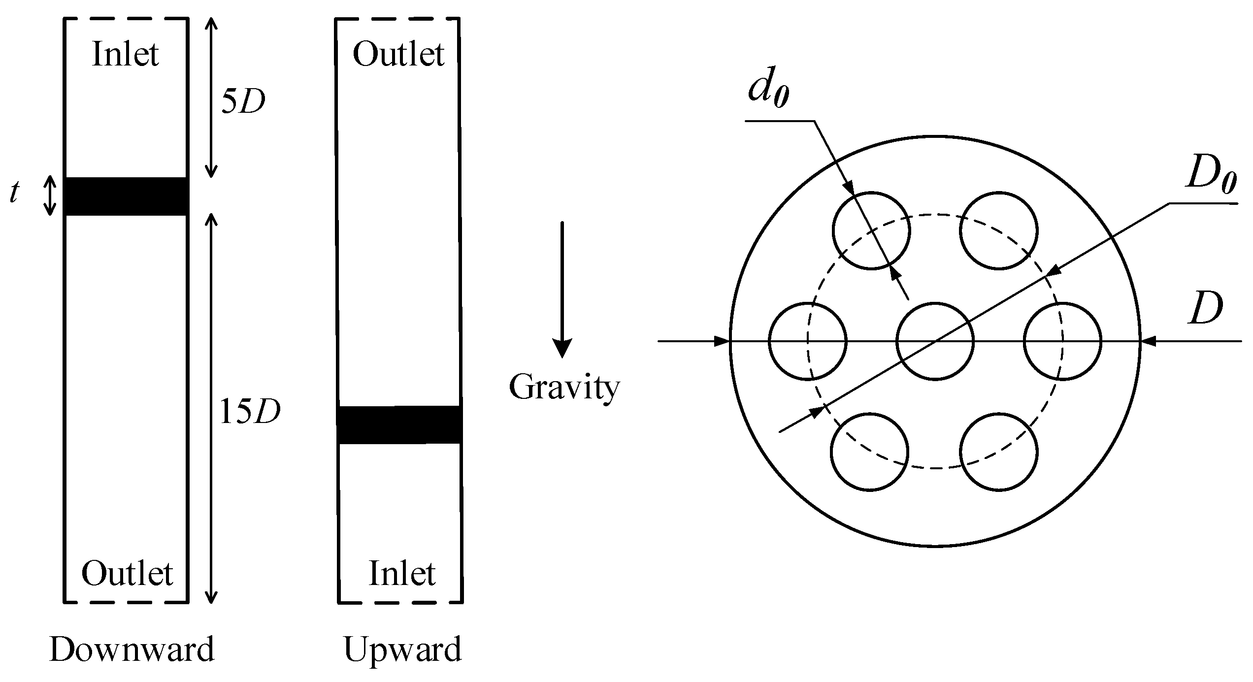
The vertical flow is divided into downward and upward flows. Figure 2 shows the studied computational domain and the two-dimensional structure of the perforated plates. To ensure that the flow fully develops and recovers, straight pipe sections with lengths of 5D and 15D are setup upstream and downstream of the perforated plate, respectively, where D = 25 mm. The thickness of the plate is t. The perforated plates used in this study have seven holes, and the diameters of the holes are all d₀. One hole is located at the center of the plate, and the remaining six holes are uniformly distributed in a circle with a diameter of D₀, where D₀ = 16 mm.

Numerical simulations of LH₂ through the perforated plates are carried out with ANSYS Fluent. The inlet and outlet of the pipe are set as velocity and pressure boundary conditions, respectively. The inner wall of the pipe is specified as walls with heat insulation. The inlet temperature of LH₂ is set to 77.36 K. Since the saturated vapor pressure of LH₂ at that temperature is 90,717 Pa, the outlet pressure is set to 200,000 Pa to ensure that the LH₂ is supercooled.

In the iterations, the coupling of pressure and velocity adopts the SIMPLE algorithm, the interpolation of pressure adopts PRESTO discretization, and the discretization of momentum, energy, and turbulence equations adopts the second-order upwind scheme. It is considered to be convergent when the residual of the continuity is less than 10⁻³, and the other convergence indexes are all less than 10⁻⁶.

3.2. Governing Equations

Currently, the study of cavitation phenomena commonly uses the homogeneous mixture method based on two-phase flow [25]. Since the thermal effect of LH₂ cavitation is not negligible [26,27], the governing equations should include the continuity equation, momentum equation, energy equation, and transport equation for the vapor volume fraction:

$${\displaystyle \frac{\partial }{\partial \mathrm{t}}}\left({\mathsf{\rho }}_{\mathrm{m}}\right)+{\displaystyle \frac{\partial }{\partial {\mathrm{x}}_{\mathrm{j}}}}\left({\mathsf{\rho }}_{\mathrm{m}}{\mathrm{u}}_{\mathrm{j}}\right)=0$$

(13)

$${\displaystyle \frac{\partial }{\partial \mathrm{t}}}\left({\mathsf{\rho }}_{\mathrm{m}}{\mathrm{u}}_{\mathrm{i}}\right)+{\displaystyle \frac{\partial }{\partial {\mathrm{x}}_{\mathrm{j}}}}\left({\mathsf{\rho }}_{\mathrm{m}}{\mathrm{u}}_{\mathrm{i}}{\mathrm{u}}_{\mathrm{j}}\right)=-{\displaystyle \frac{\partial \mathrm{p}}{\partial {\mathrm{x}}_{\mathrm{i}}}}+{\displaystyle \frac{\partial }{\partial {\mathrm{x}}_{\mathrm{j}}}}\left[\left({\mathsf{\mu }}_{\mathrm{m}}+{\mathsf{\mu }}_{\mathrm{t}}\right)\left({\displaystyle \frac{\partial {\mathrm{u}}_{\mathrm{i}}}{\partial {\mathrm{x}}_{\mathrm{j}}}}+{\displaystyle \frac{\partial {\mathrm{u}}_{\mathrm{j}}}{\partial {\mathrm{x}}_{\mathrm{i}}}}\right)\right]+{\mathsf{\rho }}_{\mathrm{m}}\overrightarrow{\mathrm{g}}+\overrightarrow{\mathrm{F}}$$

(14)

$${\displaystyle \frac{\partial }{\partial \mathrm{t}}}\left({\mathsf{\rho }}_{\mathrm{m}}{\mathrm{h}}_{\mathrm{m}}\right)+{\displaystyle \frac{\partial }{\partial {\mathrm{x}}_{\mathrm{j}}}}\left({\mathsf{\rho }}_{\mathrm{m}}{\mathrm{h}}_{\mathrm{m}}{\mathrm{u}}_{\mathrm{j}}\right)={\displaystyle \frac{\partial }{\partial {\mathrm{x}}_{\mathrm{j}}}}\left[\left({\mathsf{\lambda }}_{\mathrm{m}}+{\mathsf{\lambda }}_{\mathrm{t}}\right){\displaystyle \frac{\partial }{\partial {\mathrm{x}}_{\mathrm{j}}}}\left(\mathrm{T}\right)\right]+{\mathrm{S}}_{\mathrm{E}}$$

(15)

$${\displaystyle \frac{\partial }{\partial t}}\left(\alpha {\rho }_v\right)+{\displaystyle \frac{\partial }{\partial {\mathrm{x}}_{\mathrm{j}}}}\left(\alpha {\mathsf{\rho }}_{\mathrm{v}}{\mathrm{u}}_{v,\mathrm{j}}\right)=R$$

(16)

u_j is the velocity component of the mixed fluid, where the gas and liquid phases share the same velocity. ρ_m, μ_m, λ_m, and h_m are the density, dynamic viscosity, thermal conductivity, and enthalpy of the mixture, respectively. $\overrightarrow{\mathrm{F}}$ is the volume force. S_E is the volume heat source term caused by the phase change. R represents the net mass transfer source term.

The realizable k-ε turbulent model can better describe features such as streamline and vortex, so it has been widely used to simulate cryogenic cavitation flow [28]. It is also chosen here to simulate the LH₂ throttling process in the perforated plate.

Schnerr and Sauer [29] adopted the Rayleigh–Plesset equation for bubble dynamics to deduce an expression for the net mass transfer source term R in the following forms:

$$R=\left\{\begin{array}{c}{\mathrm{R}}_{\mathrm{g}}-{\mathrm{R}}_{\mathrm{c}}=3{\displaystyle \frac{{\mathsf{\rho }}_{\mathrm{v}}{\mathsf{\rho }}_{\mathrm{l}}}{{\mathsf{\rho }}_{\mathrm{m}}}}\alpha \left(1 - \alpha \right){\left({\displaystyle \frac{\alpha }{1 - \alpha }}{\displaystyle \frac{3}{4\mathrm{n}}}{\displaystyle \frac{1}{\mathrm{n}}}\right)}^{-{\displaystyle \frac{1}{3}}}\sqrt{{\displaystyle \frac{2}{3}}{\displaystyle \frac{{\mathrm{p}}_{\mathrm{v}}\left(\mathrm{T}\right) -\mathrm{p}}{{\mathsf{\rho }}_{\mathrm{l}}}},}\mathrm{p}\le {\mathrm{p}}_{\mathrm{v}}\left(\mathrm{T}\right)\\ {\mathrm{R}}_{\mathrm{c}}-{\mathrm{R}}_{\mathrm{g}}=3{\displaystyle \frac{{\mathsf{\rho }}_{\mathrm{v}}{\mathsf{\rho }}_{\mathrm{l}}}{{\mathsf{\rho }}_{\mathrm{m}}}}\alpha \left(1 -\alpha \right){\left({\displaystyle \frac{\alpha }{1 -\alpha }}{\displaystyle \frac{3}{4\mathrm{n}}}{\displaystyle \frac{1}{\mathrm{n}}}\right)}^{-{\displaystyle \frac{1}{3}}}\sqrt{{\displaystyle \frac{2}{3}}{\displaystyle \frac{{\mathrm{p} -\mathrm{p}}_{\mathrm{v}}\left(\mathrm{T}\right)}{{\mathsf{\rho }}_{\mathrm{l}}}}}, \mathrm{p}>{\mathrm{p}}_{\mathrm{v}}\left(\mathrm{T}\right)\end{array}\right.$$

(17)

where R_g and R_c are the mass transfer source terms related to the growth and collapse of vapor bubbles, respectively. p_v(T) is the saturated vapor pressure at temperature T, and n is the bubble number density.

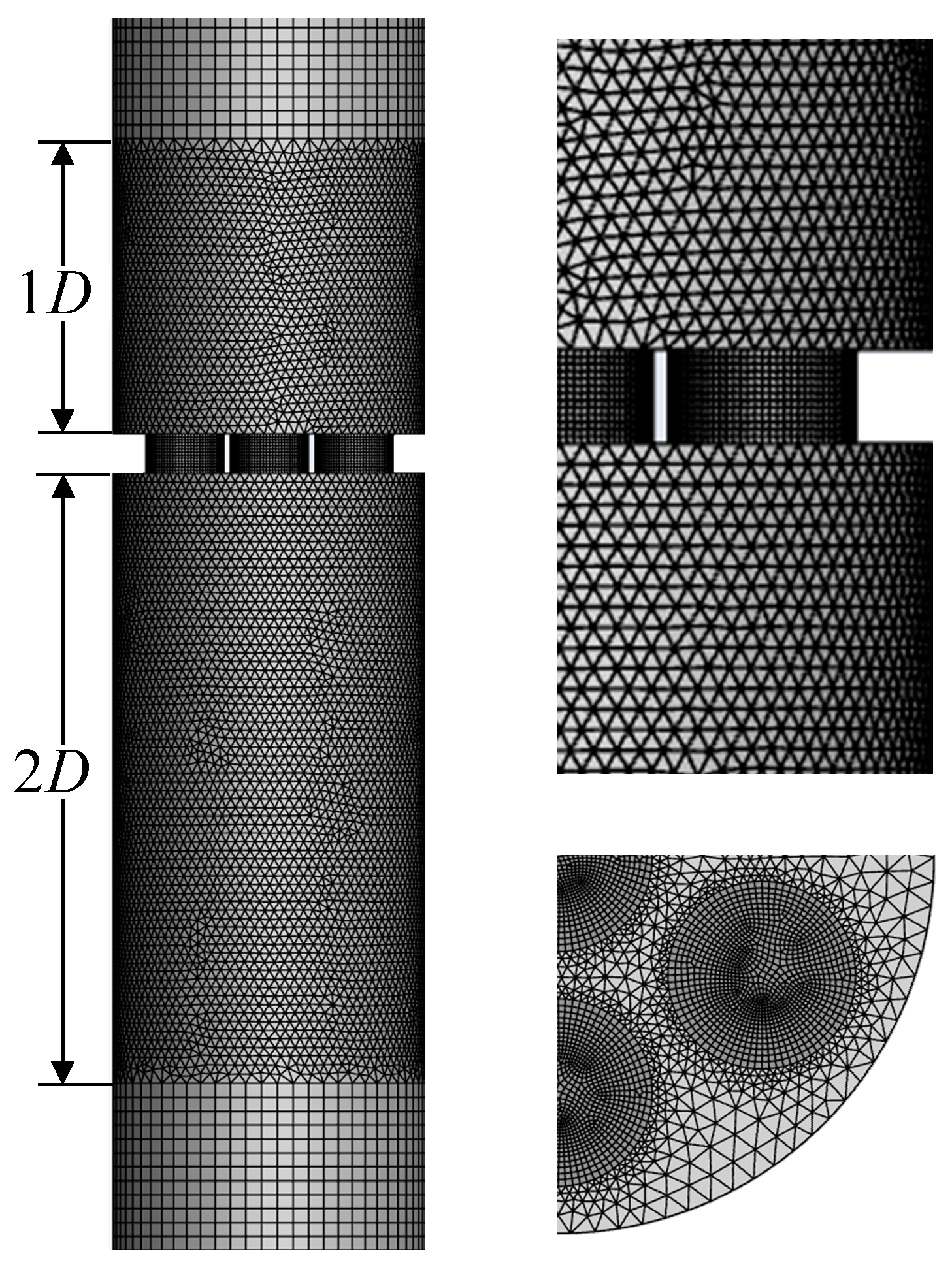
3.3. Grid Scheme

The mesh around the perforated plate is shown in Figure 3. To capture the significant pressure and velocity gradients more accurately, the grids in the 1D upstream and 2D downstream regions of the perforated plate are refined during meshing, while sparser grids are used in the other regions.

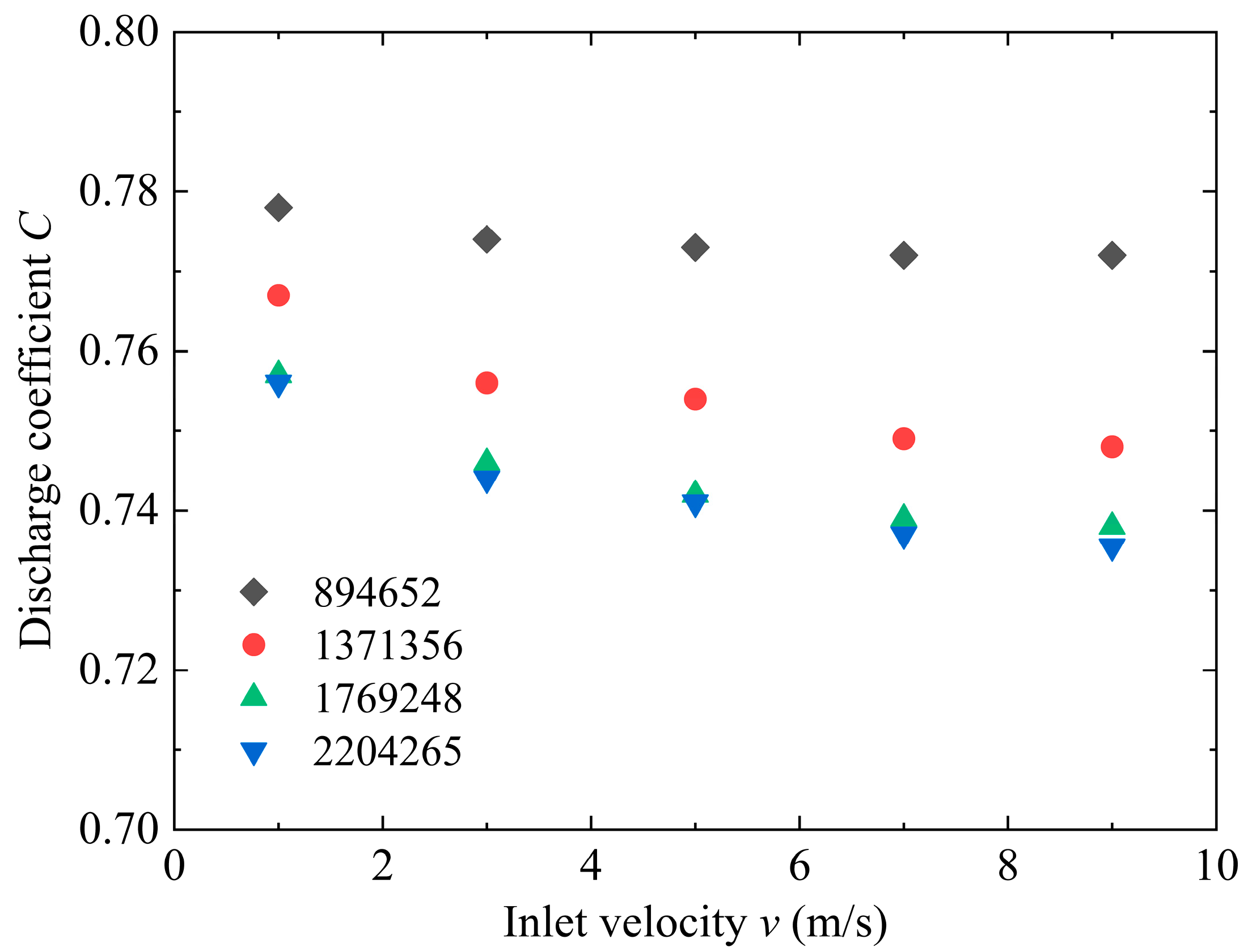
It is necessary to consider the computation time while ensuring the accuracy of the acquired data. Therefore, it is important to find a suitable number of grids. Taking the downward flow (β = 0.635, t = 3 mm) as an example, the simulation results of the C for grid numbers 894,652, 1,371,356, 1,769,248, and 2,204,265 are shown in Figure 4. When the number of grids increases from 1,769,248 to 2,204,265, the change in C is less than 0.35%. Therefore, the grid number of 1,769,248 is adopted in the following simulation.

3.4. Model Validation

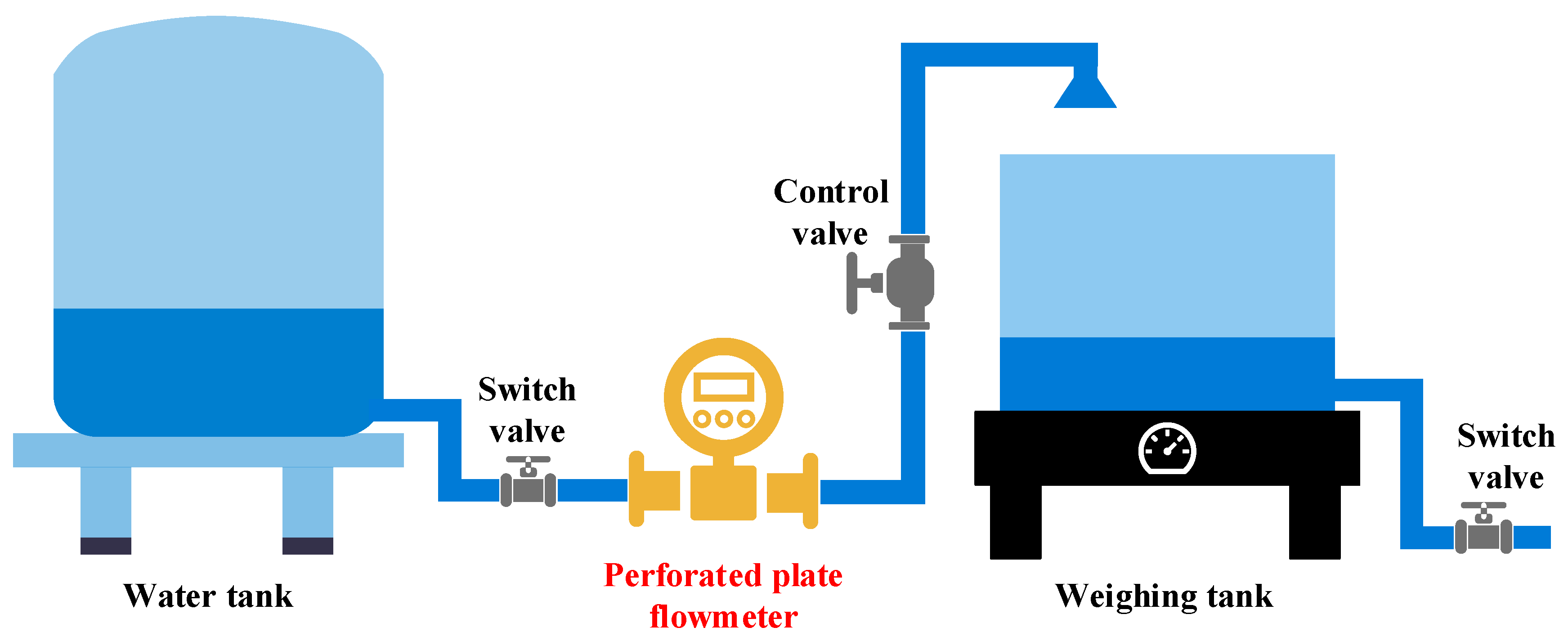
This study established an experimental system to validate the turbulence model. For the convenience of installation, horizontal flow was used for the experiments. Figure 5 shows a diagram of the experimental system. Water flows from the water tank, flows through the perforated plate flowmeter into the weighing tank. The standard flow rate is calculated by weighing the quality of the outflow water within a certain period of time. 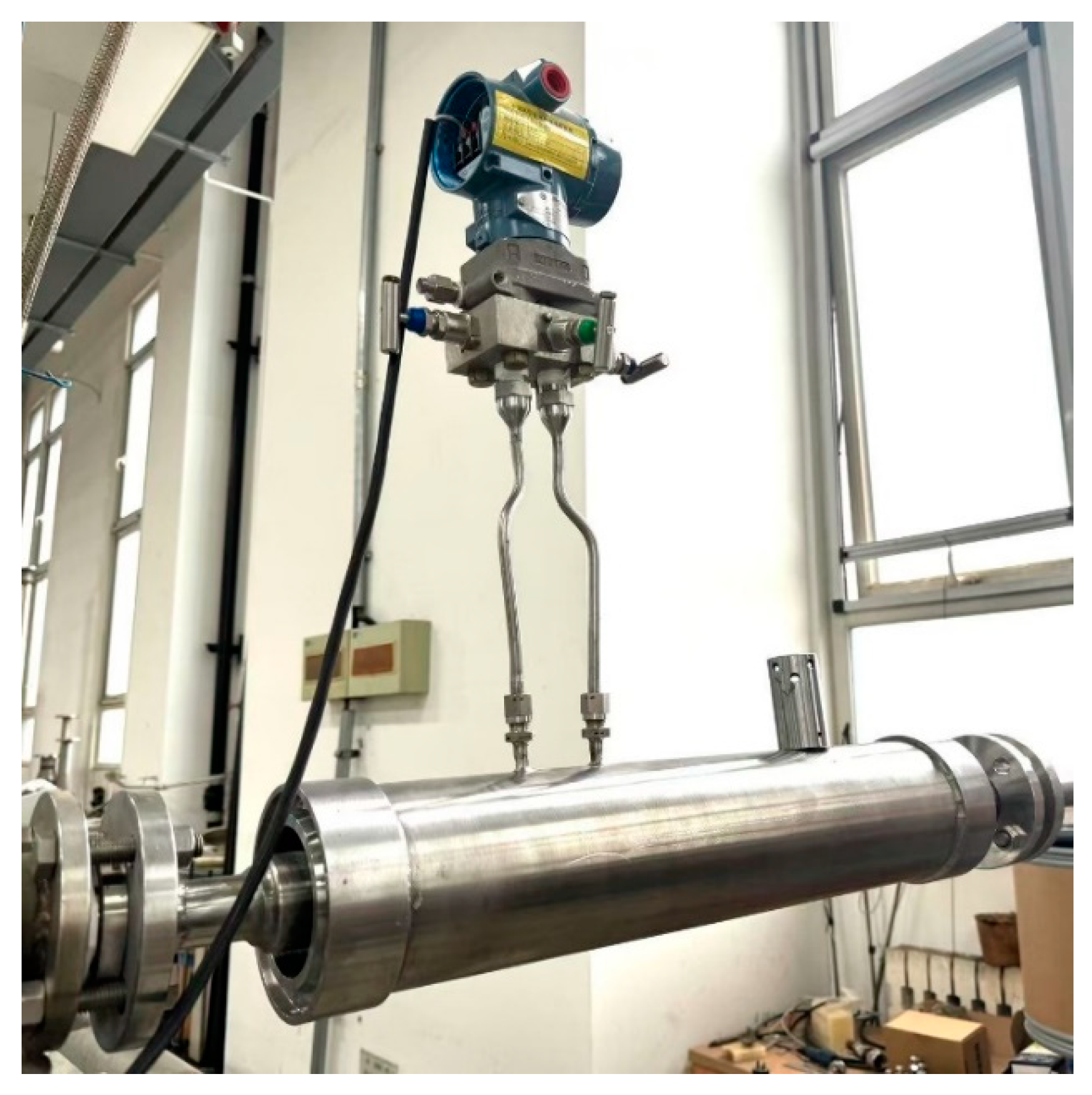Figure 6 is the photograph of the perforated plate flowmeter (t = 4 mm, β = 0.635). The differential pressure sensor is used to measure the pressure drop between the two ends of a perforated plate.

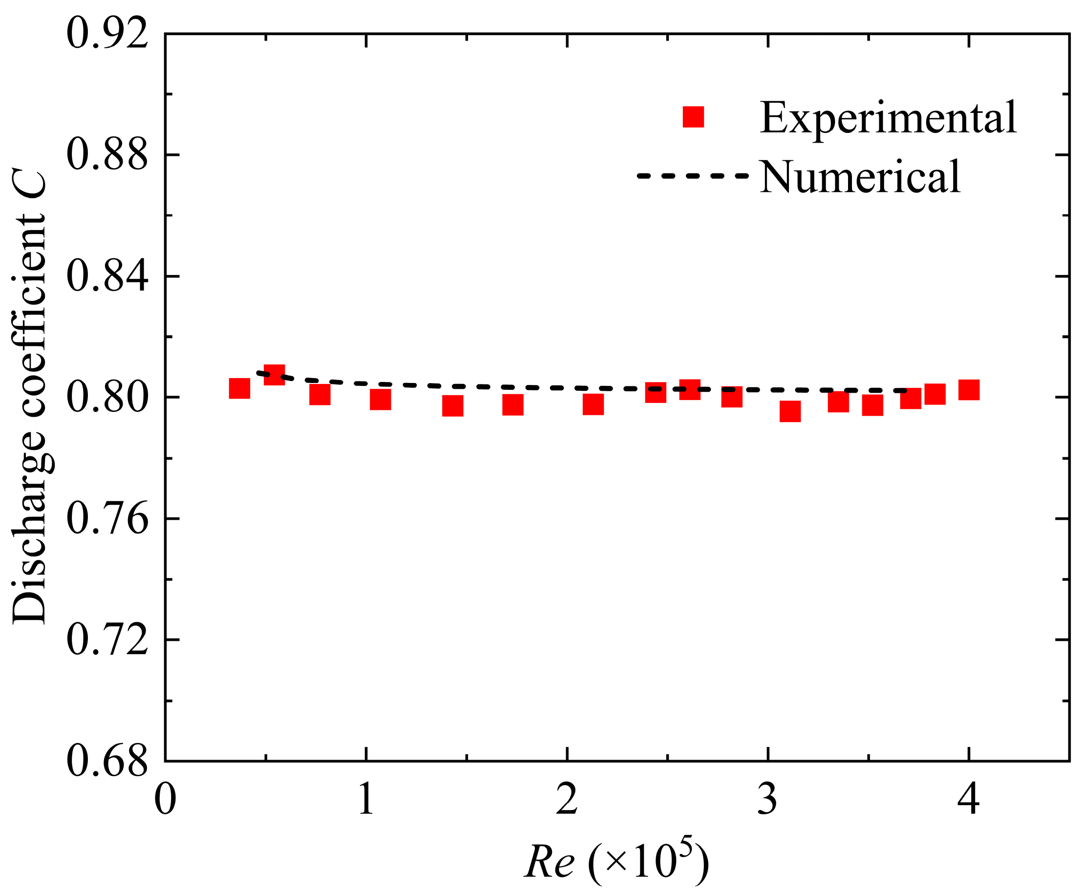
Figure 7 shows a comparison between the experimental and the numerical results of C. The experimental results of the C in the stable region are in good agreement with the numerical results, with a maximum deviation of no more than 1%. Therefore, the selected Realizable k-ε turbulence model has been validated and can be considered reliable.

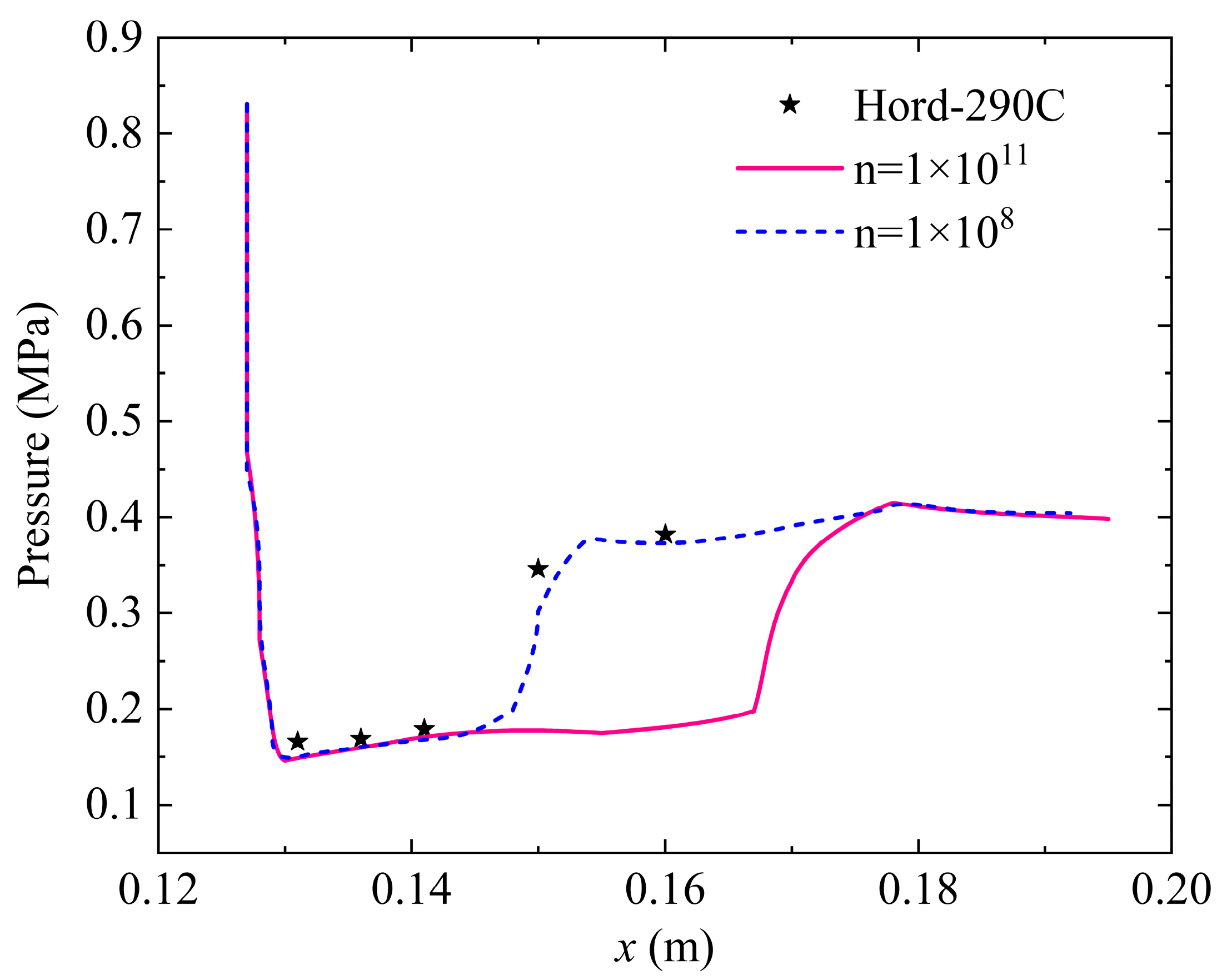
To validate the cavitation model, this paper simulates the cavitation of LN₂ passing through the hydrofoil 290C and compares it with the experimental data in Hord et al. [30] Figure 8 shows the numerical and experimental values of pressure distribution along the hydrofoil wall. Two bubble number densities, n, are considered: the default model value of 1 × 10¹¹ and the improved value of 1 × 10⁸ suggested by Zhu et al. [31] as more suitable for simulating the cavitation of cryogenic fluids. It can be seen that when n = 1 × 10⁸, the pressure distributions along the hydrofoil wall are all well consistent with the experimental data. Therefore, the following simulations will use the cavitation model with n = 1 × 10⁸.

4. Results and Discussions

4.1. The Effect of Inlet Reynolds Number

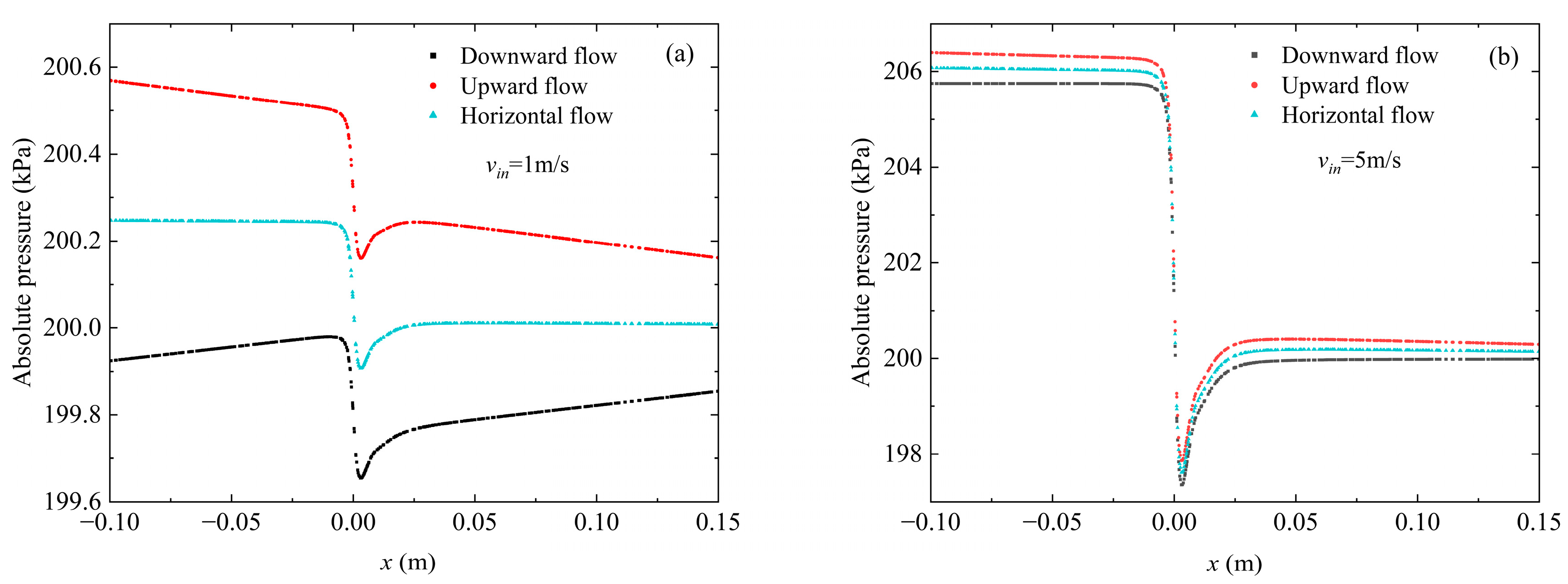
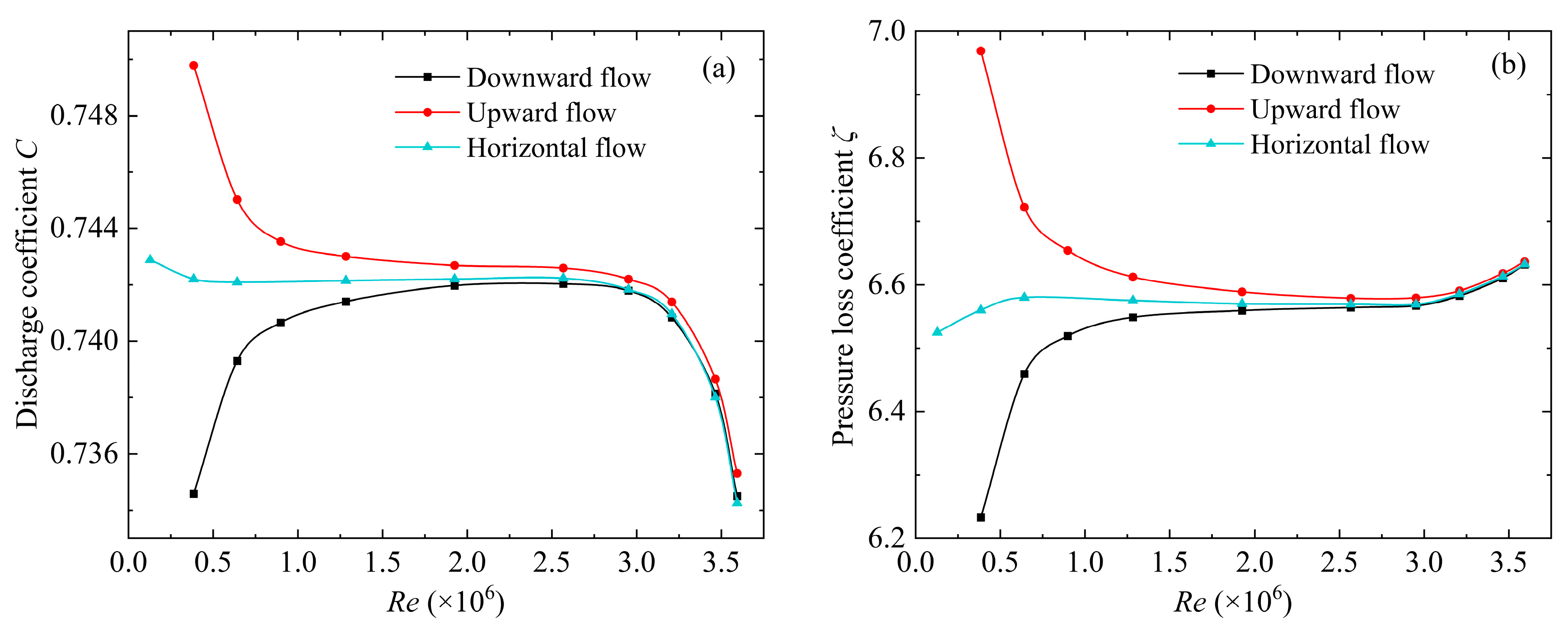
LH₂ is used to first investigate the impacts of flow direction on several typical parameters under a specific perforated plate structure (β = 0.635, t = 3 mm), including pressure, C, ζ, and vapor volume fraction.

Figure 9 shows the pressure changes along the centerline for two vertical flows and horizontal flow at different inlet velocities. At x = 0, the pressure drops due to the throttling of the perforated plate, with higher flow velocity causing a more significant pressure drop. For downward flow, gravity results in the lowest pressure at the plate being lower than that of horizontal and upward flows. In Figure 9a, it is clear that in the straight pipe of the flowmeter, the pressure variations differ significantly depending on the flow direction. Without considering pipe friction, the pressure in the horizontal flow remains constant in the straight pipe. For vertical flows, the pressure increases in the downward flow and decreases in the upward flow due to the conversion between potential and kinetic energy. For higher flow velocity in Figure 9b, although these differences still exist, the variations between different flow directions become smaller, and the pressure changes are more similar. At this point, the pressure change caused by gravity is less pronounced compared to that caused by the throttling of the plate. Overall, the influence of gravity on pressure variations diminishes as the flow velocity increases.

Figure 10 shows the variation in C and ζ with Reynolds number for different flow directions. It is also evident that in the low Reynolds number region, the difference between flow directions is pronounced, while at higher Reynolds numbers, the variations tend to coincide. In the low Reynolds number region, unlike the trends observed for horizontal flow, the C and ζ for vertical flow change in the same trend with increasing Reynolds number. According to the Formula (11), since the term $g\mathsf{\Delta }y$ is positive for downward flow, the C is reduced compared to horizontal flow, and the smaller permanent pressure loss results in a lower ζ. The opposite is true for upward flow. Additionally, the lower limit of the Reynolds number for the stable region in vertical flow is significantly higher than that in horizontal flow, leading to a smaller stable region. This indicates that vertical flow introduces greater flow instability. It can also be seen that downward flow behaves more similarly to horizontal flow.

Figure 11 shows the cavitation cloud of LH₂ under different flow directions and inlet Reynolds numbers. The cavitation region mainly occurs downstream of the perforated plate, and as the Reynolds number increases, the cavitation region expands significantly, leading to an increase in the hydrogen volume fraction. Comparing the two different vertical flows under the same inlet Reynolds number, the downward flow experiences a slightly higher velocity when reaching the plate due to the influence of gravity. This enhances turbulence and flow separation, resulting in a greater degree of cavitation.

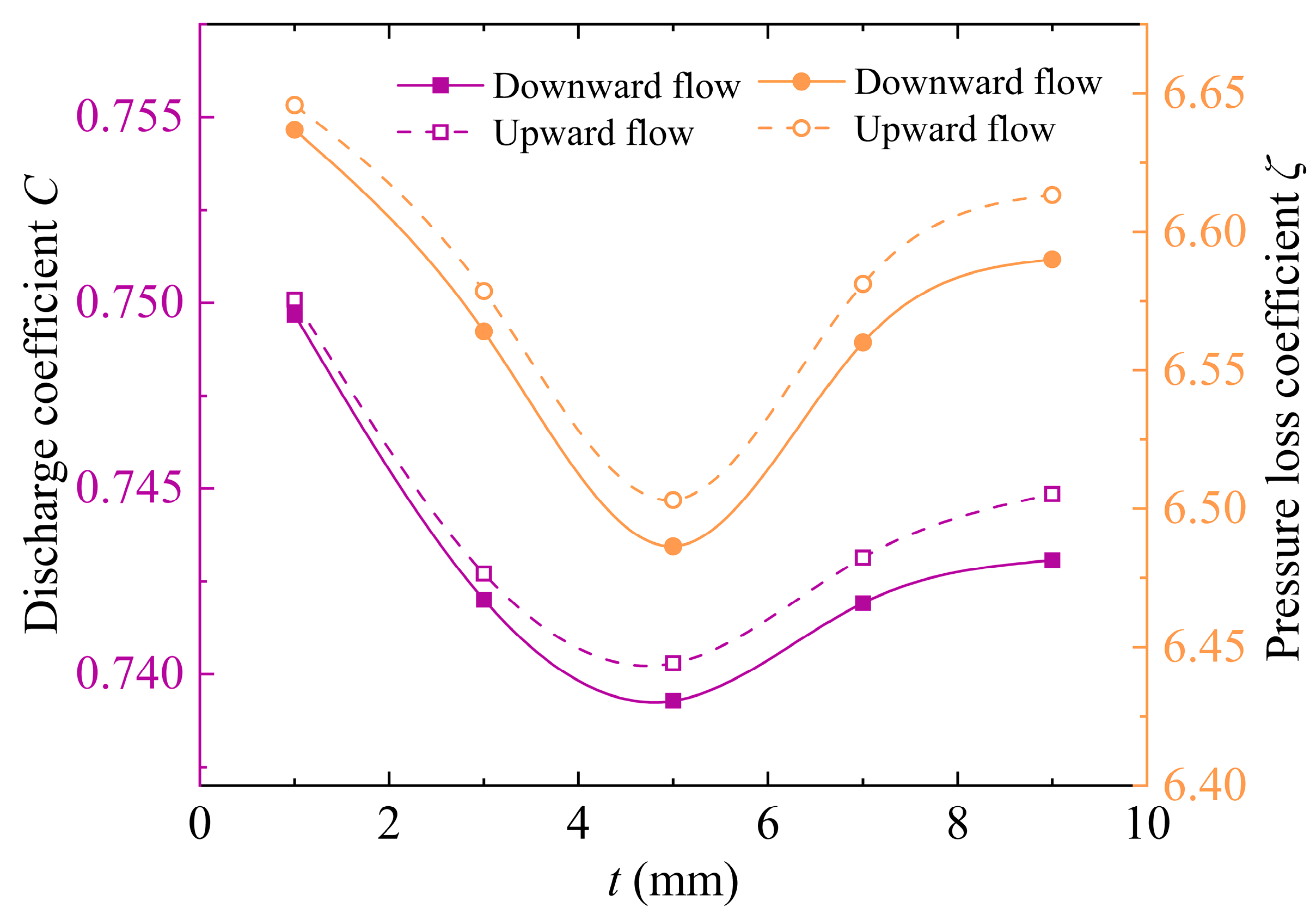
4.2. The Effect of Thickness

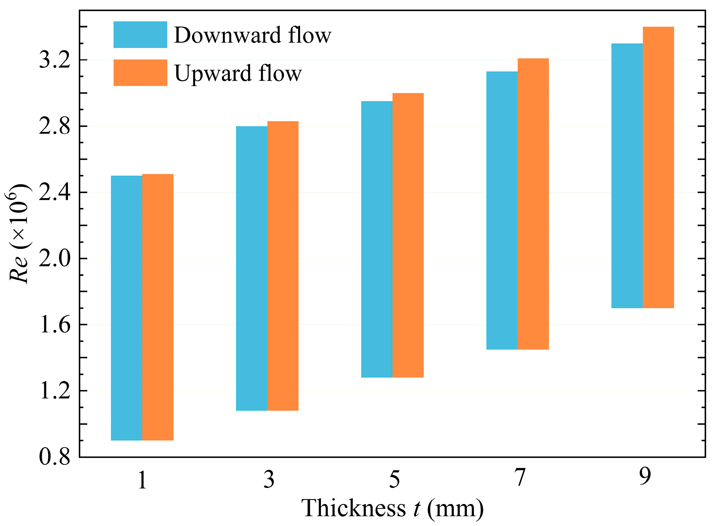
The effects of the thickness of the plate on performance parameters in vertical flow are studied based on the same equivalent diameter ratio (β = 0.635). Five thickness levels are considered: t = 1, 3, 5, 7, and 9 mm.

Figure 12 shows the variation in C and ζ with thickness, and Figure 13 shows the change in stable region with thickness. As the thickness increases, both the C and ζ initially decrease and then increase, reaching their minimum values at t = 5 mm, indicating that significant changes in flow and resistance occur around this thickness. The C and ζ for upward flow are higher than for downward flow, and this difference becomes more pronounced with increasing thickness. This suggests that although the C is higher for upward flow, overcoming gravity and causing more turbulence results in greater pressure loss. As thickness increases, the flow path becomes longer and more complex, requiring more effort to overcome gravity, which amplifies this impact. Additionally, the increase in thickness enlarges the term $\mathsf{\Delta }y$ in the Formula (11), which further increases the difference in C between upward and downward flow.

The increase in thickness shifts the stable region toward higher Reynolds numbers, though the overall range remains basically unchanged. When the thickness increases from 1 mm to 9 mm, the upper limit of the Reynolds number for stable region increases from 2.5 × 10⁶ to 3.3 × 10⁶, an increase of about 32%, indicating that the increase in thickness delays the occurrence of cavitation. Compared to upward flow, downward flow is more prone to cavitation, with a slightly higher upper limit of the Reynolds number for stable region. This difference becomes more pronounced as thickness increases, but the lower limit of the Reynolds number for the stable region remains nearly the same for both cases.

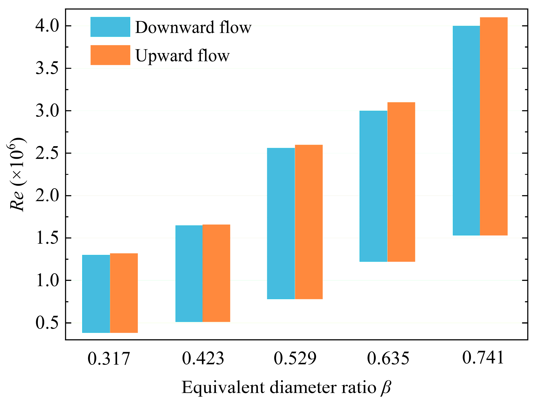
4.3. The Effect of Equivalent Diameter Ratio

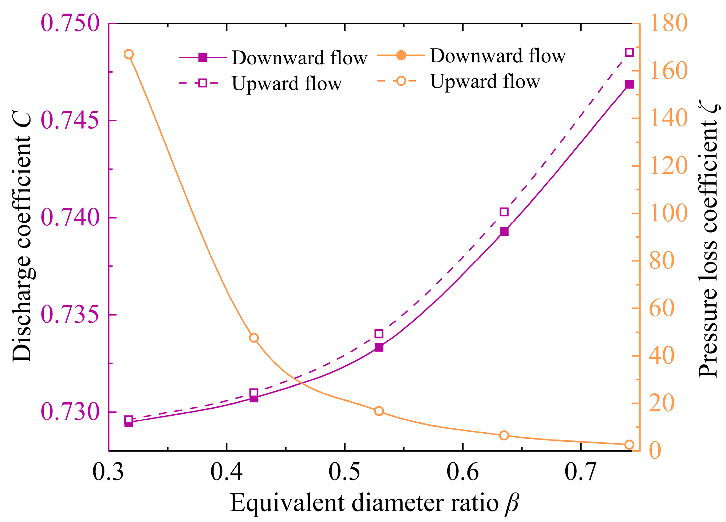
Further analysis is conducted by keeping the thickness constant (t = 5 mm) and considering the effect of the β on performance. Five β levels are studied: β = 0.317, 0.423, 0.529, 0.635, and 0.741. Figure 14 shows the variation in C and ζ with β, and Figure 15 shows the change in stable region with β. Unlike the effect of thickness, the influence of the equivalent diameter ratio on the C and ζ is the opposite. As the β increases, the C increases monotonically, while the ζ decreases monotonically. This is understandable, as a larger β implies a larger flow area, leading to a lower pressure drop and higher C. Moreover, the increase in the β not only raises the upper limit of the Reynolds number for the stable region but also extends the overall length of the stable region, indicating that systems with a larger β exhibit better flow stability. Additionally, upward flow still has a larger C, ζ, and upper limit of the Reynolds number for the stable region compared to downward flow (where the difference in ζ is less noticeable due to the small overall range on the axis). The gap between these values also widens with the increase in the β.

5. Conclusions

The flow characteristics of liquid hydrogen flowing through a perforated plate flowmeter in a vertical pipe are studied by numerical simulation under varying inlet Reynolds numbers, plate thicknesses, and equivalent diameter ratios. The focus is on the discharge coefficient, pressure loss coefficient, and stable region. It is found that due to the influence of gravity, the flow in the vertical direction exhibits different characteristics compared to the horizontal flow. The main conclusions are as follows:

(1)

When the structure is held constant, the influence of flow direction on the performance parameters of the perforated plate flowmeter diminishes with increasing Reynolds number, with the throttling effect of the perforated plate becoming predominant.

(2)

Under the influence of gravity, downward flow experiences lower pressure loss but greater flow instability, resulting in a smaller discharge coefficient, pressure loss coefficient, and lower upper limits of Reynolds numbers for stable regions. The flow characteristics of downward flow are more akin to horizontal flow. Additionally, the differences in the effects of gravity become more pronounced at larger thicknesses and greater equivalent diameter ratios.

(3)

The effective operating range of the perforated plate flowmeter can be adjusted by altering its structures. Increasing the equivalent diameter ratio or the thickness within a certain range can effectively raise the measurement upper limit of the perforated plate flowmeter and reduce pressure loss. However, when the increase in thickness exceeds a certain limit, both the discharge coefficient and pressure loss coefficient of the flowmeter will increase.