Analysis of the Impact of Photovoltaic Generation on the Level of Energy Losses in a Low-Voltage Network

Abstract

Due to the dynamic development of energy generation in photovoltaic installations, a reliable assessment of their impact on the level of energy losses in distribution networks is needed. For energy companies managing network resources, this issue has a very tangible practical aspect. Therefore, ongoing analyses of the level of electricity losses based on actual measurement data of prosumers are needed. In the paper, the influence of energy introduced by prosumer photovoltaic installations on energy losses in a low-voltage radial line is investigated. The issue is examined from three perspectives: 1. Focused on energy supplied into the low-voltage grid from photovoltaic installations; 2. the installations’ locations; and 3. the product of energy and distance from the power source. Comparative assessments are made of the examined aspects for 87 possible locations of prosumer installations in the tested low-voltage network. An analysis of energy losses is carried out both for the entire analysed network and separately for the line and the transformer. The changes in energy losses are influenced by both the power and the location of the photovoltaic installations. Based on the research findings, functions defining relative changes in energy losses in the low-voltage network are determined.

1. Introduction

The European energy sector is currently undergoing a profound transformation. This is the result of climate change resulting from combustion of fossil fuels and greenhouse gas emissions. Europe faces the restructurisation of the entire energy sector, aimed at carbon neutrality. Electricity systems should rely on clean technologies and support the decarbonisation of the economy. The development of distributed generation, including renewable energy, is inevitable. The only disputed aspect is the pace at which this process will unfold. As part of this restructurisation, more sustainable and environmentally friendly energy sources will be promoted. However, renewable energy sources pose a challenge for conventional energy systems due to difficulties in their effective integration with the grid. Therefore, it is necessary to modify the electricity infrastructure so that it is able to work with a variety of energy sources and to manage them efficiently. The dynamics of the development of renewable energy sources has a significant impact on the level of energy losses in the power grid. The increasing share of energy coming from RESs changes the nature of electricity generation, as these sources are characterised by time-varying and unpredictable energy generation. As a result there is an increasing need to ensure the reliability and sustainability of the electricity system. The power grid plays a key role in the development of the entire country, making the continuous expansion of its infrastructure and the ability to connect new zero-emission energy sources crucial. A modern energy system should facilitate the integration of innovative renewable energy sources by increasing flexibility through energy storage and local balancing. This leads to progress towards a more sustainable energy future.

Distribution System Operators (DSOs) are currently facing increasing challenges related to the dynamic development of RES installations, struggling to balance energy generation from these installations with the time-varying demand of consumers. Despite the difficult administrative and legal conditions, interest in the construction of new renewable energy sources remains high. The low price, numerous support programmes, the ease of constructing RES installations, and the economic benefits of their operation generate significant interest. Consumers are becoming prosumers, and the amount of energy they produce far exceeds their needs, resulting in energy surpluses. The capacity of prosumer installations is steadily growing and surpassed 7 GW in 2022—the envisaged target for 2030 according to the Energy Policy of Poland until 2040 [1]. Until now, electricity flowed in one direction, i.e., from the grid to the customer. However, the increasing number of RES installations necessitates transforming the grid into a bidirectional system, where energy can flow both to the consumer and back to the grid. Power grids cannot keep up with the pace of these changes, becoming a significant obstacle to rapid energy transformation. New sources have a substantial impact on voltage conditions and power flows. Further development of RESs and the increase in overproduction generated by RESs necessitate the expansion of the grid infrastructure and the implementation of new, innovative tools to manage the grid [2].

The increase in energy losses and voltage variations represent a significant issue for low-voltage networks with distributed generation. The occurrence of uncontrolled voltage rises and drops can affect the energy quality and the stability of the system. In a network with micro-sources and small installations, these changes are not only dependent on the network load, but also on the instant energy generation. Maintaining the reliability and efficiency of the network is only possible through proper planning. In order to minimise the risk of sudden voltage fluctuations, it is necessary to plan the distribution of renewable energy sources and adapt them to the load of the network concerned and the total generation. It is necessary to take into account the load on a given part of the network and the distance from the transformer. The distribution of power-generating equipment largely influences changes in power loss and voltage levels. Concentrating sources in one location has a different effect to distributing them evenly. Moreover, locating sources in close proximity to the transformer has different consequences to placing them at the backend of the network. Thorough monitoring of power flows and electricity quality analyses are required. These will make it possible to optimise the operation of the network and deliver energy with appropriate quality parameters.

The main factors contributing to the challenges of integrating renewable sources with a low-voltage network are as follows:

• Large capacity of renewable energy installations connected in an area supplied from a single MV/LV substation;
• Large distance of the installations from the supply transformer station;
• Variability and instability of renewable energy generation;
• Poor condition of the infrastructure: power grid and MV/LV transformers;
• Low energy demand during peak generation periods;
• Inadequate source control, incorrect selection of components and their parameters;
• Problems with integrating different renewable energy sources into a single branch of an LV line;
• Expansion of installations without notifying the DSO [2].

The analysis of electricity losses becomes important within the concept of distributed generation, which aims to physically locate generation sources and energy storage in close proximity to consumers. As part of distributed generation, these sources can be directly or indirectly connected to distribution networks, using installations located in households or connected to industrial networks. This flexibility in the placement of sources and storage contributes to increased reliability of the electricity system, a significant reduction in distribution losses, and enables the delivery of energy in a more efficient manner.

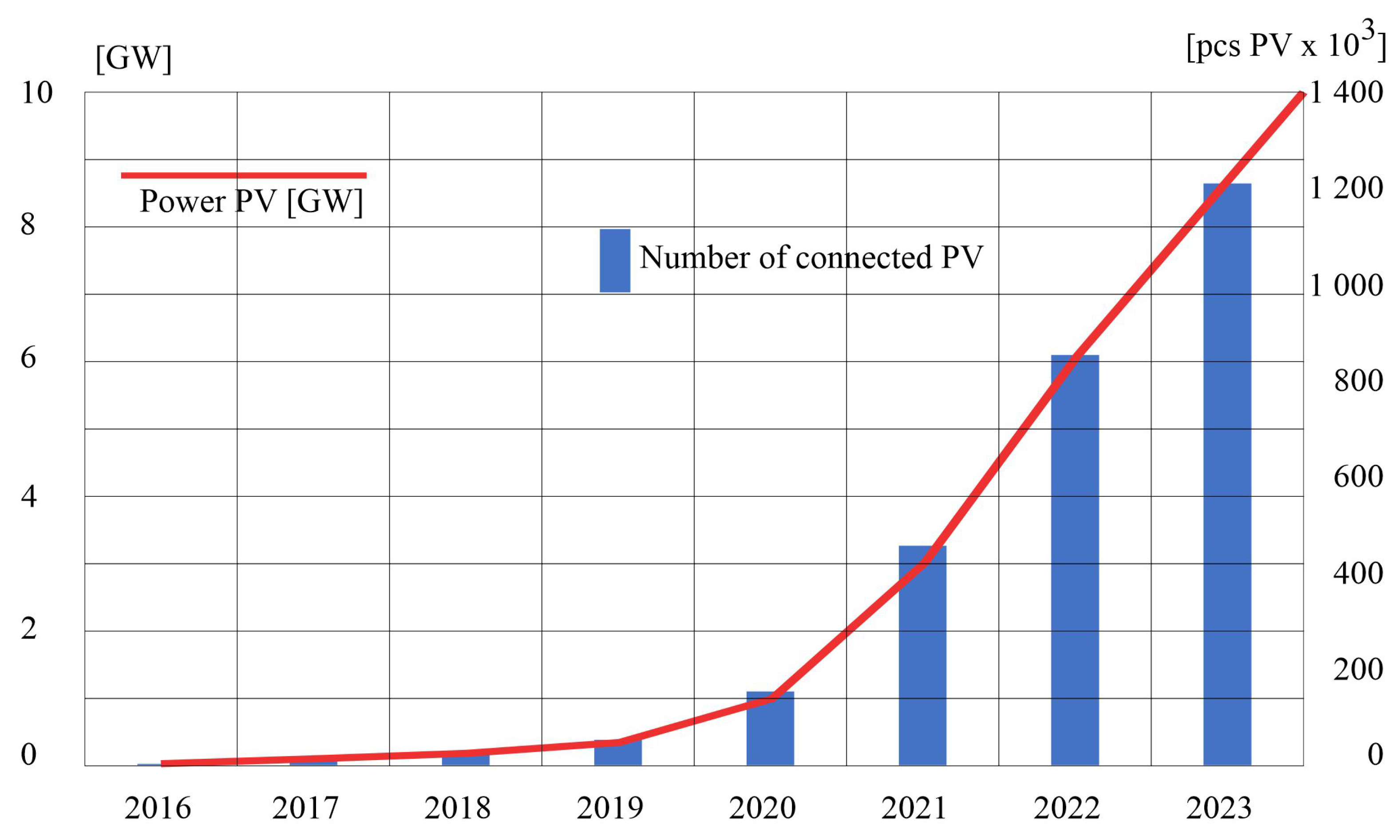
Based on the report from the Polish Society for the Transmission and Distribution of Electricity (PTPiREE) entitled “Micro-installations in Distribution Networks in Numbers—state as of the end of May 2023”, Figure 1 illustrates the growth dynamics of the number and capacity of micro-installations connected to distribution networks. These data are crucial for understanding the trends and challenges associated with the development of micro-installations and their impact on distribution networks in Poland.

Figure 1 shows the increase in both the number and total capacity of installations that occurred in Poland over the last seven years. Since 2016, a very dynamic increase in both the number and capacity of installations connected to electricity networks has been observed. The number of micro-installations in Poland increased by 297 times; simultaneously, a 309-fold increase in installed capacity took place. In January 2023, the number of installations exceeded 1.2 million, with a total installed capacity of micro-installations reaching 9.25 GW. The largest year-by-year percentage increase was observed in 2017 vs. 2016, and in 2021 vs. 2020; in both cases the growth exceeded 200%. In contrast, the smallest growth occurred in 2023 compared to 2022, with the capacity growing by about 52% and the number of installations by just under 42%. The slowdown in growth may be attributed to high inflation, and rising costs of components and loans to finance RES installations.

The topic of assessing the impact of prosumer photovoltaic generation on the distribution network is highly relevant, as evidenced by the large number of published scientific papers. In the literature concerning the impact of prosumer photovoltaic generation on low-voltage networks, several key areas of analysis can be identified. Some papers focus on issues related to energy losses (active/reactive) in LV networks, others address voltage fluctuations at the network nodes and the limitations that arise during PV operation, and some explore methods for optimising PV capacity and its location in the studied networks.

Optimisation methods for PV allocation are based on various computational techniques, often using statistical models, fuzzy set theory, artificial neural networks, hybrid algorithms combining different computational techniques such as neural networks and fuzzy logic, and particle swarm optimisation methods with elements of genetic algorithms [3,4,5,6,7,8,9]. Ref. [10] provides an interesting comparison of methods used for DG localisation applied to different test networks (IEEE bus-33, bus-69, bus-118, radial network, meshed network) and with different objectives (single objective, multi-objective, economic indices). The authors conducted an analysis of minimising energy losses and reducing voltage fluctuations as a function of PV penetration levels using, in their opinion, an efficient arithmetic optimisation algorithm (AOA) method.

In [11], the IEEE 123 Node Test Feeder was used to determine the efficiency of the distribution network (DN) and estimate energy losses at various levels of prosumer penetration. The results indicate that reducing energy losses is possible only up to a certain level of PV penetration, after which additional PV capacity increases energy losses and complicates DN operation. Lower energy losses were observed in cases of distributed PV generation compared to those concentrated in energy communities. The paper presents several approaches for the optimal deployment of distributed generation, considering capacity/energy loss minimisation and voltage stability.

The authors of [12] examined the impact of PV systems on voltage asymmetry and energy losses in a real residential distribution network in Thailand. Based on simulation studies using the DIgSILENT Power Factory software, the authors determined the variation in energy losses, concluding that higher PV generation capacities can be tolerated in phases with higher load density.

In [13], the impact of prosumer installations on the operation of several variants of low-voltage network structures presented by the authors was discussed. The issue was illustrated with a computational example that considered factors such as the size and location of prosumer installations and the cross-sections of power cables.

The first part of ref. [14] presents an analysis of the distribution of introduced energy density and energy losses in low- and medium-voltage lines and LV/MV transformers. The second part presents a reliability assessment of the same distribution areas based on an analysis of the distributions of the System Average Interruption Duration Index (SAIDI) and the System Average Interruption Frequency Index (SAIFI) for planned and unplanned outages. The analysis of data from real networks was carried out using non-parametric methods with kernel density estimators (KDEs).

In view of the subject matter of this paper, the work of [15] should be taken into account. It presents two scenarios for the development of the energy distribution system: In the first, consumers are distributed prosumers with small-scale photovoltaic installations (a few kW); and in the second consumers become prosumers through membership in energy communities (EComs), which serve as single-node medium-capacity sources (up to a few MW). The study estimated energy losses for 36 different variants (in both scenarios of distribution network development). The analysis was carried out for an IEEE bus-33 test network. Simulations were carried out for actual annual PV load and generation profiles, using energy network data and annual meteorological data, determining the operationally feasible levels of PV penetration for distributed prosumers and energy community prosumers (EComPs). In the context of the material further presented, it is worth mentioning ref. [16], which discusses the potential of Advanced Metering Infrastructure (AMI) systems, which have become an important element of the distribution system. The AMI system is a source of annual data collected from prosumers for the analysis of energy losses in the network under study.

The main contributions of this study are as follows:

• The NEPLAN software was used to calculate the operation of an actual distribution network at different levels of photovoltaic penetration, using actual hourly profiles of both energy consumption and photovoltaic generation.
• Comparative assessments were made for 87 variants of the deployment of prosumer installations in the analysed low-voltage network. The issue was examined in three aspects: in relation to the energy introduced into the low-voltage network from photovoltaic installations, their location, and the product of energy and distance from the power source.
• For the variants studied, functions defining relative changes in energy losses in the analysed network were presented.
• The influence of energy introduced by prosumer photovoltaic installations on energy losses was examined both for the entire analysed network and separately for the line and the transformer.

The rest of the paper is organised as follows. Section 2 presents a description of a real radial-type low-voltage network. The assumptions made and the scope of the research carried out are specified. Section 3 presents the developed network model in the NEPLAN program, the applied analysis method together with assumptions, and a list of 87 variants of network calculations. Section 4 discusses the results. The basic statistical measures of relative energy losses in lines and transformers are given. The photovoltaic penetration levels for which minimal energy losses occur in the tested network for both lines and transformers are estimated. Functions of changes in relative energy losses are determined in the following aspects: energy introduced to the low-voltage network from photovoltaic installations, their location, and the product of energy and distance from the power source. Finally, the conclusions are presented.

2. Radial Low-Voltage Network with Distributed Generation

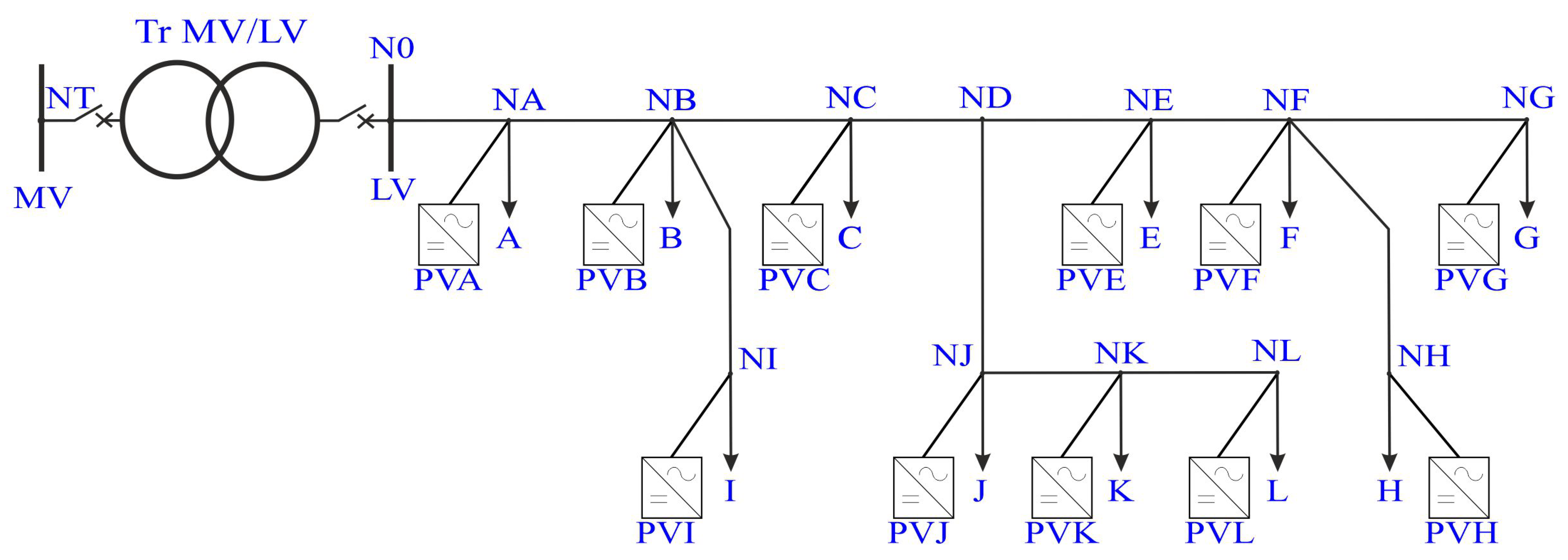
The analysis of the impact of energy introduced by prosumer photovoltaic installations on energy losses in a low-voltage line was carried out based on measurement data from a real network operating in southern Poland, constituting part of the national DN. The analysed low-voltage network is shown in Figure 2.

The network under study includes a 40 kVA Tr MV/LV transformer station (Tr), from which a 50 mm² AFL-8 low-voltage overhead line is routed, and eleven consumers. Each consumer on this network is metered with a meter that allows for reading their consumption profile, averaged over an hourly period.

The transformer data from the nameplate is as follows: $S_N$ = 40 kVA, $U_{NH}$ = 15.75 kV, $U_{NL}$ = 0.4 kV with a regulation of ±3 × 2.5 , $U_R$ = 2.55%, corresponding to $P_o$ = 1020 W, short-circuit voltage $U_k$ = 4%, and no-load losses $P_j$ = 82 W. The transformer connection group is Dyn5.

The unit parameters of the 50 mm² AFL-8 overhead line, with a nominal rated voltage of 0.4 kV, are as follows: unit resistance R1 = 0.606 Ω/km, unit reactance X1 = 0.39 Ω/km, unit conductance B1 = 2.959 μS/km, and maximum current Imax = 150 A.

Table 1. Lengths of individual sections of the 50 mm² AFL-8 overhead line.

Network Node Name	Length of Line Section [m]
N0–NA	$L_{0A}$ = 180.75
NA–NB	$L_{AB}$ = 187.35
NB–NC	$L_{BC}$ = 136.25
NC–ND	$L_{CD}$ = 181.28
ND–NE	$L_{DE}$ = 230.03
NE–NF	$L_{EF}$ = 260.03
NF–NG	$L_{FG}$ = 167.53
NB–NI	$L_{BI}$ = 117.68
ND–NJ	$L_{DJ}$ = 65.75
NJ–NK	$L_{JK}$ = 163.25
NK–NL	$L_{FL}$ = 184.50
NF–NH	$L_{FH}$ = 294.23

shows the lengths of the individual sections of the 50 mm² AFL-8 overhead line. The total length of the $L_C$ line is 2168.63 metres. The lengths of the individual sections between the nodes, marked according to Figure 2, are shown in Table 1.

The prosumers in the analysed network operate under the rules applicable in Poland for installations registered by 31 March 2022, according to the so-called net metering system. This billing system is based on energy balancing—for every 1 kWh of energy fed into the grid, the prosumer receives 0.8 kWh. Therefore, the capacities of the connected photovoltaic installations for each consumer were selected based on their actual energy consumption profiles.

Table 2. Photovoltaic installation capacity, annual energy consumption, and power factor for each consumer.

Consumer Designation	Annual PV Energy Production [MWh]	Annual Energy Consumption [MWh]	Average Power Factor—cos $\mathit{\phi }$
A	$E{G}_A$ = 2885.31	$E{C}_A$ = 2404.42	−0.95
B	$E{G}_B$ = 5676.05	$E{C}_B$ = 4730.04	0.92
C	$E{G}_C$ = 3909.73	$E{C}_C$ = 3258.11	−0.94
E	$E{G}_E$ = 4156.33	$E{C}_E$ = 3463.61	0.92
F	$E_{G}F$ = 4010.71	$E{C}_F$ = 3342.26	0.91
G	$E{G}_G$ = 3809.44	$E{C}_G$ = 3174.54	0.93
H	$E{G}_H$ = 2615.56	$E{C}_H$ = 2179.64	0.94
I	$E{G}_I$ = 2775.29	$E{C}_I$ = 2312.74	0.90
J	$E{G}_J$ = 2452.24	$E{C}_J$ = 2043.54	−0.94
K	$E{G}_K$ = 5717.57	$E{C}_K$ = 4764.64	0.92
L	$E{G}_L$ = 5676.01	$E{C}_L$ = 4730.01	0.90
Sum	$\sum EG$ = 43,684.24	$\sum EC$ = 36,403.53	−

presents the annual energy consumption and the average power factor for each consumer, marked with the symbols A, B, C, E ÷ L, as well as the photovoltaic installation capacities marked as PVA, PVB, PVC, PVE ÷ PVL.

The analysis presented in this paper assumes the installation of 3-phase inverters that ensure symmetrical current generation in each phase (thus eliminating additional losses due to generation asymmetry). The capacity of each installation is tailored to the annual electricity consumption of a given consumer to ensure that the annual energy production from the photovoltaic panels exceeds the annual energy demand of the respective consumer by 20%. 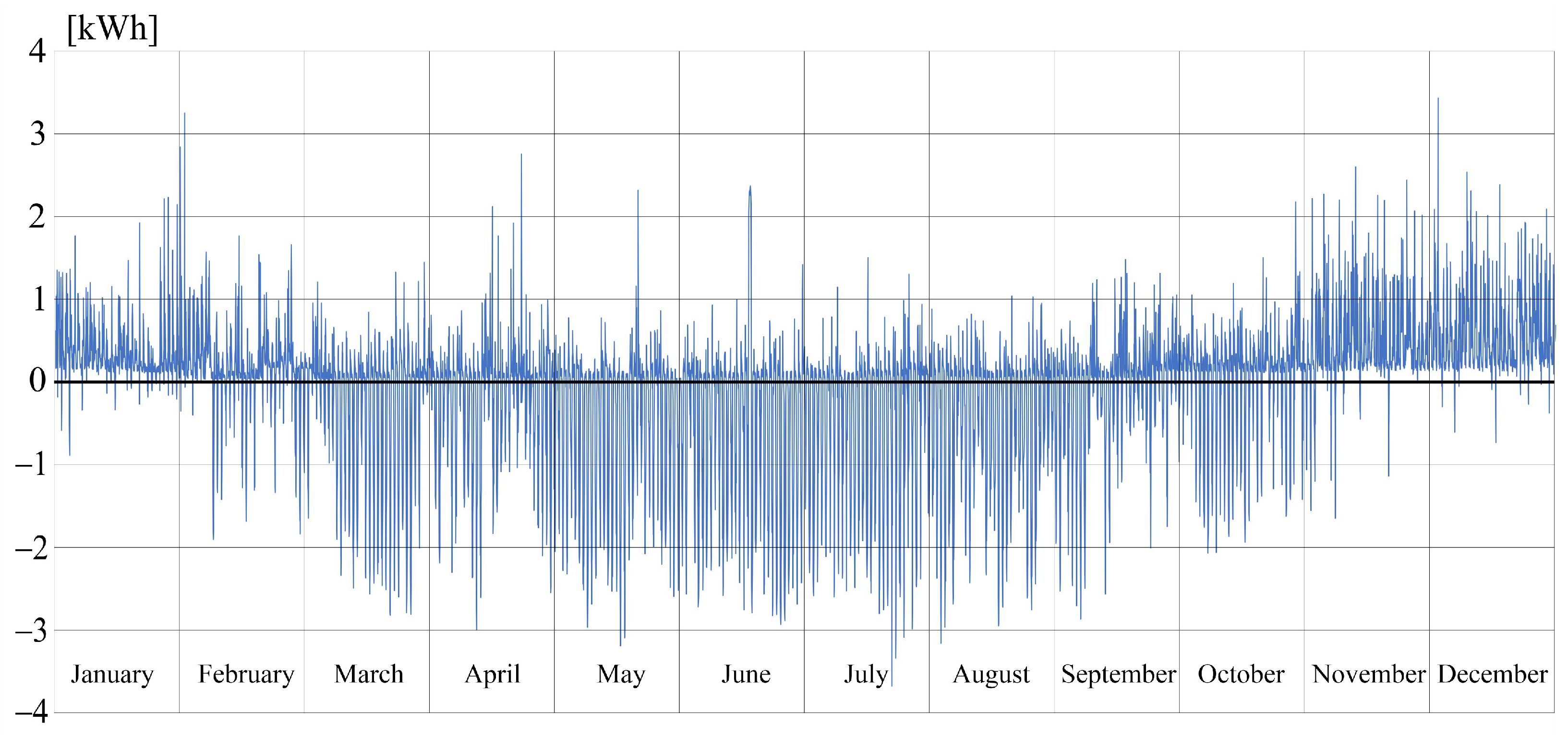Figure 3 shows the difference between the energy consumed and the energy produced by the PVC photovoltaic installation for prosumer C at specific hours of the year, expressed in kWh.

As can be seen in Figure 3, during the summer and the same part of the spring and autumn periods, the amount of energy produced by PVC significantly exceeds the energy demand of prosumer C.

3. Methods

NEPLAN software was used to analyse the distribution network under study at specific levels of distributed generation penetration. The NEPLAN software is designed for the analysis, planning, optimisation, and simulation of electricity systems [17].

The Newton method [18] (also known as the Newton–Raphson method or the tangent method) is used to determine power flows. The classic problem of calculating power flows involves determining the voltage magnitude and phase angle at busbars, as well as the flowing active and reactive power in the lines under specific conditions at each node in the network. In order to analyse the power losses under different network operating conditions, a model of the network was developed in NEPLAN. The extended Newton–Raphson method was used for the calculations. The programme settings assumed a convergence mismatch of e⁻⁰⁰⁵ and a maximum of 50 iterations.

The NEPLAN module Load Flow with Load Profiles enables a sequence of power distribution calculations over a specified time period using data prepared in external files (provided via the object name).

Before each power flow calculation, the active and reactive power of consumers and generators are loaded from the measurement data. The measurement data are entered into NEPLAN in the form of an ASCII file, where header lines for each profile must be defined. An example format of the data file header is shown below:

$$\begin{array}{c}\hfill \mathrm{Year}\mathrm{Month}\mathrm{Day}\mathrm{t}[\mathrm{hh}:\mathrm{mm}]\mathrm{P}\left[\mathrm{MW}\right]\mathrm{Q}\left[\mathrm{MVAr}\right]\end{array}$$

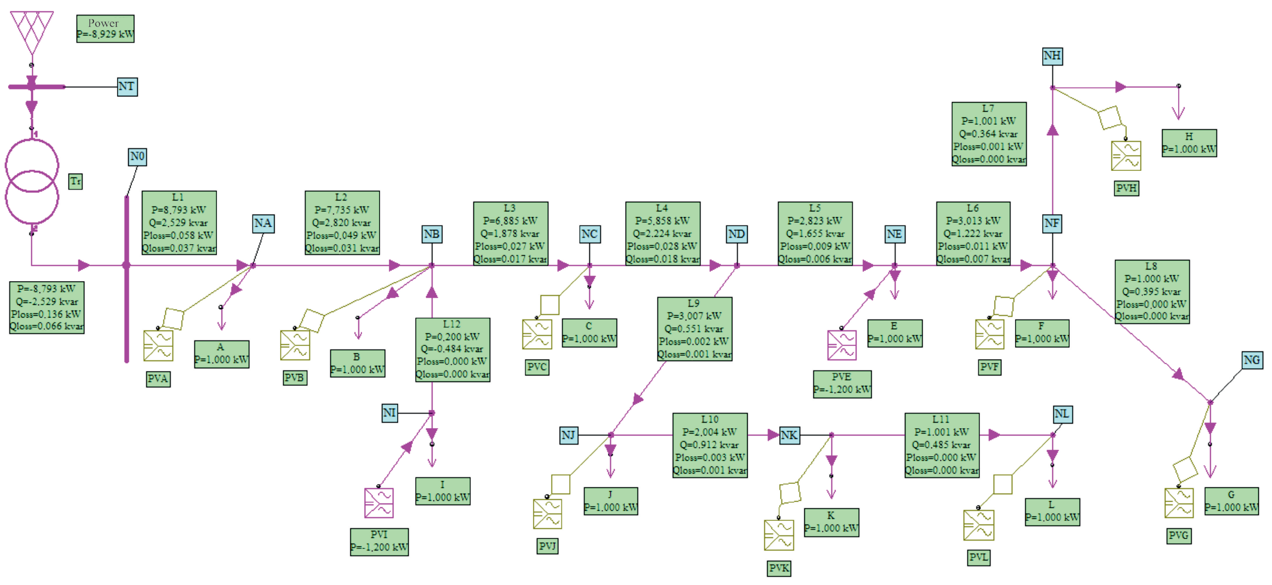
Each load or generation element requires its own file. The name of such a file must be the name of the element with the extension .txt (e.g., A.txt). This method permits the definition of measurement data for an unlimited number of days. The developed network model is shown in Figure 4.

In the analysis carried out in accordance with the data read from external files, an n-fold analysis of Load Flow with Load Profiles is performed for each variant of active PV system configuration. Based on the loaded data from 00:00 on 1 January 2022 to 23:00 on 31 December 2022, calculations of the flows in this network are performed. At 1-h intervals, on the basis of consumer profiles and generation profiles of photovoltaic installations, currents, voltages, and power flows in the studied network are calculated for each analysed period, and the results are saved in the designated file.

Thus, the analysis presented involves an 8760-fold analysis based on real measurement data from 2022, loaded into the NEPLAN software. The study was carried out for a varying number of active PV installations distributed within the network, according to the following number of variants (k ranging from 0 to 11 variants with one, two or three PVs active up to a variant where all PV installations are active). The number of analysed variants n for a given amount k of active PVs is presented in the following list:

0.

without active PVs (k = 0);

1.

with one active PV (k = 1, for which 11 variants were analysed);

2.

with two active PVs (k = 2, for which 11 variants were analysed);

3.

with three active PVs (k = 3, for which 11 variants were analysed);

4.

with four active PVs (k = 4, for which 10 variants were analysed);

5.

with five active PVs (k = 5, for which 10 variants were analysed);

6.

with six active PVs (k = 6, for which 9 variants were analysed);

7.

with seven active PVs (k = 7, for which 8 variants were analysed);

8.

with eight active PVs (k = 8, for which 7 variants were analysed);

9.

with nine active PVs (k = 9, for which 5 variants were analysed);

10.

with ten active PVs (k = 10, for which 3 variants were analysed);

11.

with each consumer having a PV installation (k = 11).

In total, the paper presents an analysis of the operation of the studied network for n = 87 variants for the deployment of 11 PV installations.

4. Results

In order to determine the impact of individual PV installations on energy losses in the low-voltage network, the energy losses in the $\Delta E_L$ line, in the $\Delta E_T$ transformer, and the total losses in the $\Delta E_N$ line and transformer were calculated for different PV installation variants, based on the number of installations and their distribution points in the analysed network. The energy losses in the analysed network without PV installations were as follows: for the entire overhead line, 478.03 kWh, denoted as $\Delta E_{L0}$; for the transformer, 855.82 kWh, denoted as $\Delta E_{T0}$ (of which 718.23 kWh were transformer no-load losses); and total network losses for the entire analysed network ($\Delta E_{N0}$) of 1333.85 kWh.

Table A1. Energy losses expressed in kWh, in total for the $\Delta E_N$ line and transformer, in the $\Delta E_T$ transformer, and in the $\Delta E_L$ lines, for connected photovoltaic installations in individual network variants.

k = 1	A	B					C				E				F					G		H					I				J				K					L
$\Delta E_N$	1310.89	1280.65					1282.13				1267.09				1265.19					1267.17		1281.87					1299.37				1288.55				1253.90					1280.55
$\Delta E_T$	844.88	838.53					841.63				840.77				840.95					841.35		845.06					844.57				845.60				836.30					839.36
$\Delta E_L$	466.01	442.12					440.50				426.32				424.24					425.82		436.80					454.81				442.94				417.61					441.18
k = 2	AB	AG					BE				BI				CE					CG		FG					GH				JK				KL					EI
$\Delta E_N$	1277.76	1256.69					1255.86				1271.86				1251.26					1247.16		1261.13					1255.44				1245.57				1300.25					1251.48
$\Delta E_T$	837.20	836.39					836.66				835.29				835.58					835.11		834.49					835.64				832.80				835.54					835.33
$\Delta E_L$	440.56	420.30					419.20				436.57				415.68					412.05		426.64					419.80				412.78				464.71					416.16
k = 3	ABC	ACF					AGK				BFK				CEG					CEL		CFG					CHJ				FGH				HIL					IKL
$\Delta E_N$	1279.36	1251.28					1246.60				1276.84				1268.07					1315.47		1273.57					1241.53				1289.82				1271.15					1314.93
$\Delta E_T$	841.98	837.20					835.39				843.05				837.12					845.10		836.43					833.88				833.97				836.81					839.76
$\Delta E_L$	437.38	414.07					411.22				433.78				430.95					470.37		437.14					407.65				455.85				434.34					475.17
k = 4	ABCE		ABKL					ACIJ					AEIJ				BCEF				BEGK				CEFG				CFIL					EHIJ					GHIL
$\Delta E_N$	1302.65		1388.00					1256.23					1249.33				1336.63				1354.73				1347.17				1333.13					1253.22					1317.76
$\Delta E_T$	855.19		868.38					836.83					836.80				857.56				858.86				846.64				851.56					834.88					843.96
$\Delta E_L$	447.46		519.62					419.40					412.53				479.07				495.87				500.53				481.57					418.35					473.80
k = 5	ABCEF		ABCGI					ABEHK					ACGJL				AEHIJ				AGHIL				BCEFK				BCEKL					BEFIJ					CGHIL
$\Delta E_N$	1372.55		1324.33					1359.76					1365.28				1267.90				1343.25				1455.61				1559.07					1343.27					1383.47
$\Delta E_T$	875.02		863.39					869.83					862.98				842.04				856.44				885.12				902.60					859.64					860.29
$\Delta E_L$	497.52		460.94					489.93					502.30				425.86				486.81				570.49				656.47					483.63					523.18
k = 6	ABCEFG			ABFHJL					ABFIKL					ABGJKL					ACEGIJ				AEGHIL					BCEFGK					BCEFJK					BEGIJK
$\Delta E_N$	1491.44			1467.46					1546.87					1550.95					1347.63				1456.96					1610.10					1531.41					1469.47
$\Delta E_T$	899.77			892.45					914.67					908.74					864.25				879.38					913.56					901.60					888.33
$\Delta E_L$	591.67			575.02					632.20					642.20					483.38				577.58					696.54					629.81					581.14
k = 7	ABCEFGH				ABCGJKL					ACEGIJL						ACEHIKL					ACGHIKL					BCEFGJK						BCFGJKL					BEFHIJK
$\Delta E_N$	1599.99				1685.19					1543.09						1615.94					1599.92					1705.46						1812.46					1582.75
$\Delta E_T$	919.58				946.59					907.50						920.53					915.77					933.84						953.85					910.00
$\Delta E_L$	680.40				738.60					635.60						695.41					684.15					771.62						858.61					672.75
k = 8	ABCEFGHI					ABCFGIJK						ABCFHIJL						ABEFGIKL						ACEGHIJL						AEFGHJKL						BCEFGJKL
$\Delta E_N$	1674.23					1656.06						1660.12						1920.73						1651.41						1896.20						2051.63
$\Delta E_T$	943.91					950.45						950.64						995.94						928.68						950.01						1001.25
$\Delta E_L$	730.31					705.62						709.48						924.79						722.73						946.20						1050.38
k = 9	ABCEFGHIJ							ABCGHIJKL									ACEGHIJKL								BCEFGHJKL									CEFGHIJKL
$\Delta E_N$	1766.42							1900.33									1910.05								2227.56									2091.39
$\Delta E_T$	967.15							1003.79									980.87								1032.36									989.03
$\Delta E_L$	799.27							896.54									929.17								1195.20									1102.36
k = 10	ABCEFGHIJK													ABCEFGHJKL														BCEFGHIJKL
$\Delta E_N$	2028.69													2318.73														2344.40
$\Delta E_T$	1029.17													1077.44														1069.05
$\Delta E_L$	999.52													1241.29														1275.35
k = 11	ABCEFGHIJKL
$\Delta E_N$	2442.76
$\Delta E_T$	1117.74
$\Delta E_L$	1325.02

(Appendix A) summarises the energy losses, divided into $\Delta E_T$ transformer losses, $\Delta E_L$ line losses, and total losses in the $\Delta E_N$ transformer and lines, expressed in kWh for various numbers of installations k (from 1 to 11) and their different installation points.

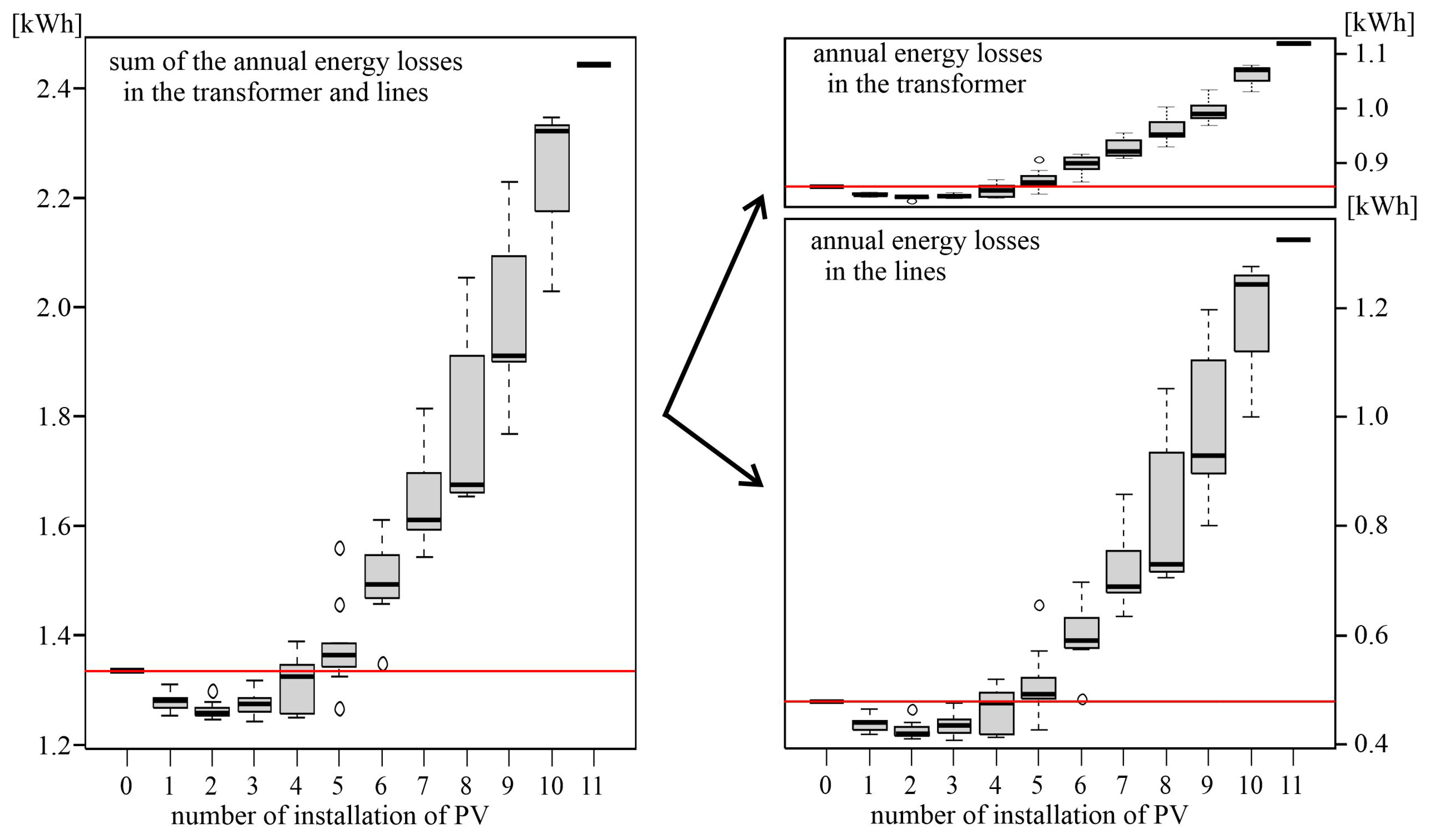
Figure 5 presents the total energy losses as well as a breakdown of energy losses in the line and transformer depending on the number of PV installations in the network. The calculations were performed in the R environment [19].

The study reveals that the difference in energy losses depends on three factors: the number of PV installations, the energy injected into the network from the PV installations, and their connection points.

As shown in Table A1 and Figure 5, integrating up to three PV installations into the network resulted in a reduction in energy losses in every case. The minimum energy losses in the studied network occurred when three PVs were active. As can be seen in Figure 5, the variations in losses in the network under study were mainly dependent on line losses, with a relatively smaller impact of transformer loss variation.

Figure 5 also highlights two outliers: the first occurs when PV installations are placed at five points (BCEKL). The energy losses for this case are very high, and this is due to the fact that the total energy generated by PVs at these points is the highest. The second outlier occurs when PV installations are placed at six points (ACEGIJ), resulting in low energy losses due to the fact that the total energy generated by consumers is the lowest in the analysed network.

In the following part of the paper, each of the n analysed variants (from 1 to 87) is evaluated and compared to the network’s state without PV installations. Further calculations and graphs are presented as relative values compared to the network state without PV installations, denoted by the subscript 0 in the formulae.

Relative energy losses for the entire network were determined for each variant n according to the following formula:

$${RCEL}_{Nn}={\displaystyle \frac{\Delta E_{Nn}}{\Delta E_{N0}}},$$

(1)

where ${RCEL}_{Nn}$—relative losses in the network for variant n; $\Delta E_{Nn}$—network losses in kWh for variant n; $\Delta E_{N0}$—network losses without PV installations, equal to 1333.85 kWh.

Table 3. Basic statistical measures $RCE{L}_N$ for individual variants of network energy losses (k—number of active photovoltaic installations).

k	1	2	3	4	5	6	7	8	9	10	11
Median	0.96	0.94	0.95	0.99	1.02	1.12	1.21	1.26	1.43	1.74	1.83
Mean	0.96	0.95	0.96	0.99	1.03	1.12	1.23	1.34	1.48	1.67	1.83
Maximum	0.98	0.97	0.99	1.04	1.17	1.21	1.36	1.54	1.67	1.76	1.83
Minimum	0.94	0.93	0.93	0.94	0.95	1.01	1.16	1.24	1.32	1.52	1.83

summarises the median, mean, maximum, and minimum values of relative network energy losses $RCE{L}_N$ for k connected PV installations compared to energy losses without PV.

Relative line energy losses for each variant n were determined from the following formula:

$${RCEL}_{Ln}={\displaystyle \frac{\Delta E_{Ln}}{\Delta E_{L0}}},$$

(2)

where ${RCEL}_{Ln}$—relative losses in the line for variant n; $\Delta E_{Ln}$—line losses in kWh for variant n; $\Delta E_{L0}$—line losses without PV installations, equal to 478.03 kWh.

Table 4. Basic statistical measures $RCE{L}_L$ for individual variants of line energy losses (k—number of active photovoltaic installations).

k	1	2	3	4	5	6	7	8	9	10	11
Median	0.92	0.88	0.91	1.00	1.03	1.24	1.44	1.53	1.94	2.60	2.77
Mean	0.92	0.88	0.91	1.00	1.03	1.24	1.44	1.53	1.94	2.60	2.77
Maximum	0.97	0.97	0.99	1.09	1.37	1.46	1.80	2.20	2.50	2.67	2.77
Minimum	0.87	0.86	0.85	0.86	0.89	1.01	1.33	1.48	1.67	2.09	2.77

summarises the median, mean, maximum, and minimum values of relative line energy losses $RCE{L}_L$ for k connected PV installations compared to energy losses without photovoltaics.

Additionally, relative transformer energy losses for each variant n were determined from the following formula:

$${RCEL}_{Tn}={\displaystyle \frac{\Delta E_{Tn}}{\Delta E_{T0}}},$$

(3)

where ${RCEL}_{Tn}$—relative losses in the transformer for variant n; $\Delta E_{Tn}$—transformer losses in kWh; $\Delta E_{T0}$—transformer losses without PV installations, equal to 855.82 kWh.

Table 5. Basic statistical measures $RCE{L}_T$ for individual variants of transformer energy losses (k—number of active photovoltaic installations).

k	1	2	3	4	5	6	7	8	9	10	11
Median	0.98	0.98	0.98	0.99	1.01	1.05	1.08	1.11	1.16	1.25	1.31
Mean	0.98	0.98	0.98	0.99	1.01	1.05	1.08	1.12	1.16	1.24	1.31
Maximum	0.99	0.98	0.99	1.01	1.05	1.07	1.11	1.17	1.21	1.26	1.31
Minimum	0.98	0.97	0.97	0.98	0.98	1.01	1.06	1.09	1.13	1.20	1.31

summarises the median, mean, maximum, and minimum values of relative transformer energy losses $RCE{L}_T$ for k connected PV installations compared to energy losses without active PV installations.

With the installation of PVs for only one consumer, the reduction in relative energy losses ranged from 0.94 to 0.98, with a greater reduction observed for lines (the median change was 0.92) compared to the transformer (median of 0.98). This is related to the fact that no-load losses, which are constant, account for almost 84% of the transformer’s energy losses during passive operation. It is also important to note that a higher reduction in energy losses is achieved when the photovoltaic installation is placed as far from the transformer as possible.

The highest reduction in energy losses in the analysed network was obtained when PV installations were connected to three consumers at nodes CHJ, with a reduction of 0.93 $\Delta E_{N0}$, and to two consumers at nodes JK, with a reduction of 0.94.

When PVs were connected to four consumers, energy loss reduction occurred in 55% of the analysed cases, with a maximum reduction of 0.95. When PVs were installed at consumers AEIJ, energy losses increased to 1.04 $\Delta E_{N0}$. When PVs were installed for five consumers, energy loss reduction was only achieved in two cases, with a maximum reduction of 0.95 (PV installed at AEHIJ). Energy loss increased to 1.17 when PVs operated for consumers BCEKL. When PVs were installed for more than 50% of the consumers in the line, energy losses increased. When PV installations were active for all consumers, network losses rose to 1.83 $\Delta E_{N0}$ (even up to 2.77 $\Delta E_{N0}$ in the line alone).

As previously mentioned, the difference in energy losses depends on three factors: the number of PV installations, the energy injected into the network from the PV installations, and their connection points.

In order to analyse the second factor—the energy introduced into the network from photovoltaic installations—a coefficient $RGC$ was defined to determine the share of energy introduced from PVs relative to the energy consumed by consumers for each research variant, as defined by the formula:

$$RG{C}_n={\displaystyle \frac{\sum E{G}_n}{\sum EC}},$$

(4)

where $RG{C}_n$—coefficient for the share of energy introduced from PVs relative to the energy consumed by consumers in variant n; $\sum E{G}_n$—sum of energy introduced from PVs for variant n of network operation; $\sum EC$—sum of annual energy consumed by connected consumers, equal to 36,403.53 MWh.

Next, the relative changes in energy losses for the transformer and line as a function of the $RGC$ coefficient were determined for each n variant.

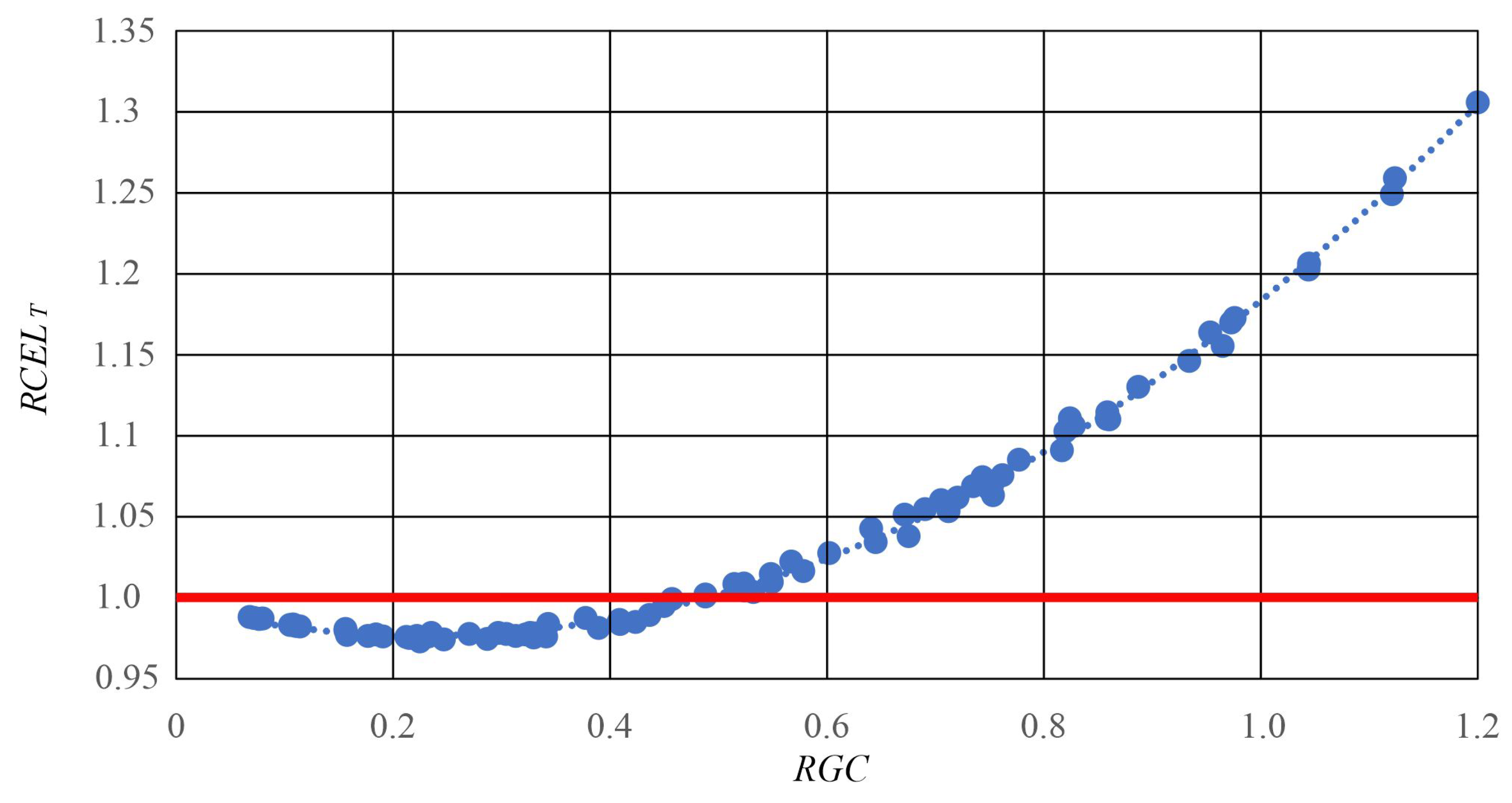
Figure 6 shows the relative changes in transformer energy losses as a function of energy introduced from PVs compared to the total energy consumed by consumers.

For the relationship shown, a function given by the following polynomial was determined:

$$RCE{L}_T=0.3489·RG{C}^2-0.1604·RGC+0.995,$$

(5)

where $RCE{L}_T$—relative energy losses in the transformer; $RGC$—energy introduced from PVs relative to the energy consumed by consumers connected to the line.

The Pearson correlation coefficient is 0.999, and the function is significant at a 0.01 significance level. If the energy introduced from photovoltaic installations does not exceed 0.489 of the energy consumed by consumers, energy losses in the transformer will not increase. When the energy introduced from PVs accounts for about 0.23 of the energy consumed by consumers, the energy losses in the transformer will be at their lowest.

Figure 7 shows relative changes in line energy losses as a function of energy introduced from PVs compared to the total energy consumed by consumers.

For the relationship shown, a function given by the following polynomial was determined:

$$RCE{L}_L=2.2579·RG{C}^2-1.1496·RGC+1.023,$$

(6)

where $RCE{L}_L$—relative energy losses in the line; $RGC$—energy introduced from PVs divided by the energy consumed by consumers connected to the line.

The Pearson correlation coefficient is 0.999, and the function is significant at a 0.01 significance level. If the energy introduced from photovoltaic installations does not exceed 0.488 of the energy consumed by consumers, energy losses in the line will not increase. When the energy introduced from PVs accounts for about 0.255 of the energy consumed by consumers, energy losses in the line will be at their lowest.

Energy losses also depend on the distance at which PV installations are connected. Therefore, for each network operation variant, the value $RL$ was calculated, representing the sum of distances of installed PV installations from the transformer relative to the total circuit length. This indicator is described by the following formula:

$$R{L}_n={\displaystyle \frac{\sum L_n}{\sum L_C}},$$

(7)

where $R{L}_n$—coefficient for the distance of PV to the transformer for variant n; $\sum L_n$—sum of distances of installed PV installations measured from the transformer for variant n of network operation; $L_C$—total circuit length, equal to 2168.63 metres.

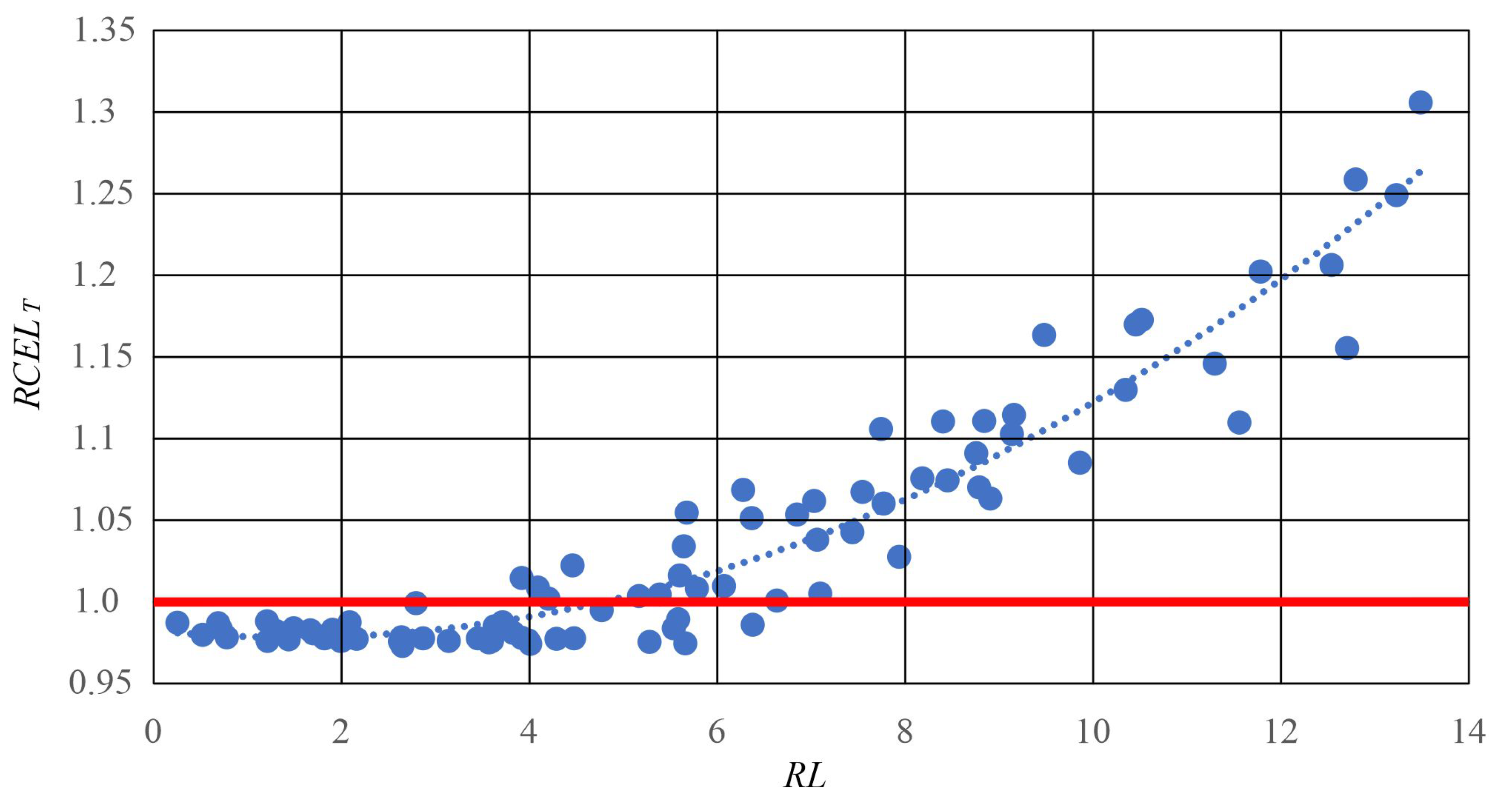
The relationship between changes in energy losses as a function of the distance of PV installations from the feed point for the transformer is shown in Figure 8.

For the relationship shown, a function given by the following polynomial was determined:

$$RCE{L}_T=0.002·R{L}^2-0.0057·RL+0.983,$$

(8)

where $RCE{L}_T$—relative energy losses at the transformer; $RL$—sum of distances of PV installations from the line feed point to the total length of the line.

The Pearson correlation coefficient for the determined function is 0.954 (significant at a 0.01 significance level). The correlation is very high, but lower than when considering the energy introduced into the line by the PV installation. This is logical because the location of the PV installation does not affect the energy flowing through the transformer.

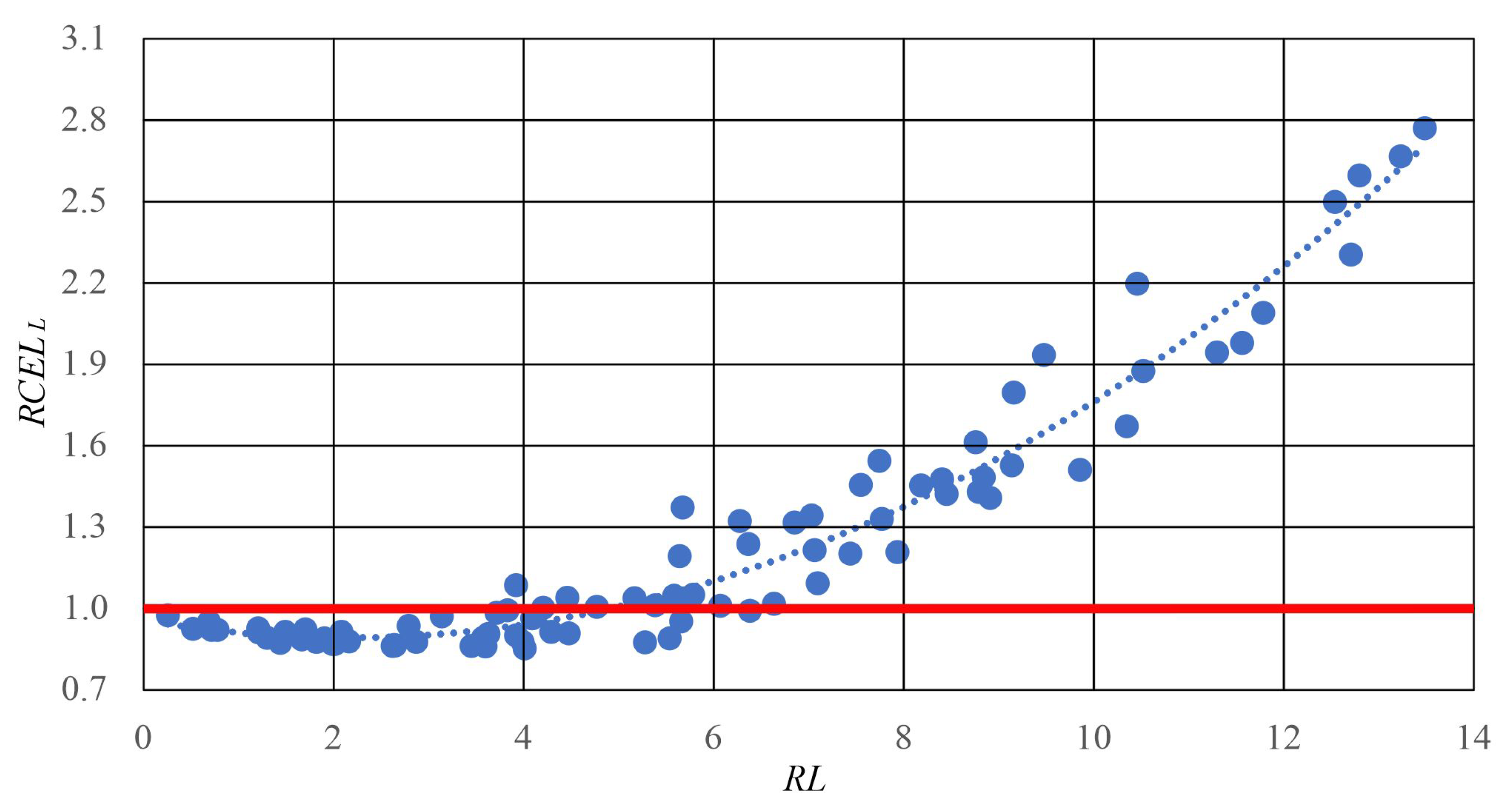
Similarly the relationship between changes in energy losses as a function of the distance of PV installations from the feed point for the line is shown in Figure 9.

For the relationship shown, a function given by the following polynomial was determined:

$$RCE{L}_L=0.0141·R{L}^2-0.0606·RL+0.9573,$$

(9)

where $RCE{L}_L$—relative energy losses in the line; $RL$—the sum of the distances of PV installations from the line feed point to the total length of the line.

The Pearson correlation coefficient was in this case 0.974 (significant at a 0.01 significance level). According to the conducted research, if the sum of distances of photovoltaic installations from the transformer does not exceed 4.88 times the total length of the track, energy losses in the line will not increase. The minimum of the function occurs when the sum of distances of PV installations from the transformer represents 2.12 times the total line length.

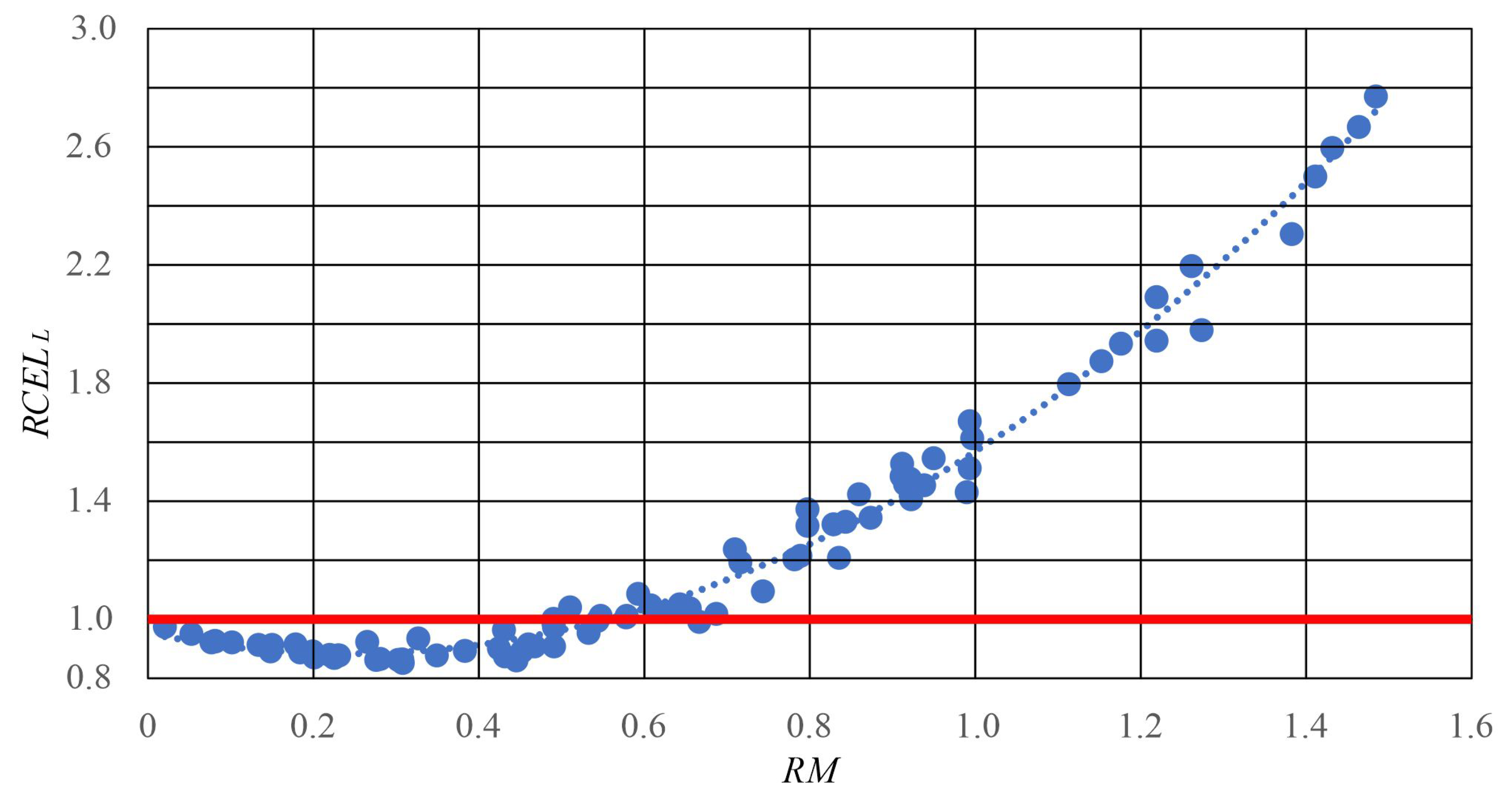
The analysis therefore shows that energy losses in the line depend on both the energy introduced from PVs and the length of the track. Therefore, for each network operation variant, the value RM was calculated, representing the sum of the product of energy introduced from PVs at successive installation points and the distance of feed sections to the PV installation point relative to the product of the total annual energy consumed by consumers and the total circuit length.

$$R{M}_n={\displaystyle \frac{\sum E{G}_n·L_n}{L_C\sum EC}},$$

(10)

where $R{M}_n$—summation coefficient of moments for variant n; $\sum E{G}_n$—sum of energy introduced from PVs for variant n of network operation; $\sum L_n$—sum of distances of installed PV installations measured from the transformer for variant n of network operation; $\sum EC$—sum of annual energy consumed by connected consumers; $L_C$—total circuit length.

The calculation results are presented in Figure 10.

For the relationship shown, a function given by the following polynomial was determined:

$$RCE{L}_L=1.1895·R{M}^2-0.5745·RM+0.9529,$$

(11)

where $RCE{L}_L$—relative energy losses in the line; $RM$—sum of the product of energy introduced from PVs at successive installation points and the distance of feed sections to the PV installation point to the transformer.

The Pearson correlation coefficient in this case is 0.993, and the function is significant at a 0.01 significance level. If the sum of moments of length and energy produced from PVs does not exceed 0.55 times the product of circuit length and energy consumed by consumers, energy losses in the line will not increase. When the sum of moments of length and energy produced from PVs represents 0.24 times the product of circuit length and energy consumed by consumers, energy losses in the line will be at their lowest.

5. Conclusions

The analysis of the impact of photovoltaic installations on energy losses in a low-voltage network was conducted in three aspects: for the entire analysed network, and separately for the line and the transformer. The paper examined the impact of the energy introduced into the network from PV installations, the location of generation sources, and the product of energy and the distance from the power source (the MV/LV transformer). The study shows that the amount of energy introduced into the network from PVs has the greatest impact on energy losses. When each prosumer contributes 120% of the energy drawn by consumers, energy losses in the lines will begin to increase when the energy from PVs exceeds 48.8% of the energy consumed by the consumers; for the transformer, this threshold is 48.9% The lowest energy losses will occur when the energy introduced from PV installations equals 25.5% of the energy consumed by the consumers. Energy losses are reduced by 6.7% in this case. Although less significant, the location of generation sources also plays an important role. The farther the PV installations are located from the transformer, the greater the reduction in energy losses.

Functions defining relative changes in energy losses depending on the amount of energy introduced from PVs, for the line and transformer, and the location (distance) of the PV generation connection and the product of energy and distance for LV lines are presented. Based on them, relative energy losses can be estimated, but it should be remembered that these equations were determined for a specific case. Therefore, changes in energy losses will be an estimate, not a specific quantity.

It should be noted that the analysed network did not take into account the impact of energy storage, heat pumps, or electric vehicle chargers. The authors’ future research will also take into account their impact on the operational aspects of the power system.