Reliability Model of Battery Energy Storage Cooperating with Prosumer PV Installations

Abstract

The energy transition toward low-carbon electricity systems has resulted in a steady increase in RESs. The expansion of RESs has been accompanied by a growing number of energy storage systems (ESSs) that smooth the demand curve or improve power quality. However, in order to investigate ESS benefits, it is necessary to determine their reliability. This article proposes a four-state reliability model of a battery ESS operating with a PV system for low-voltage grid end users: households and offices. The model assumes an integration scenario of an ESS and a PV system to maximize autoconsumption and determine generation reliability related to energy availability. The paper uses a simulation approach and proposes many variants of power source and storage capacity. Formulas to calculate the reliability parameters—the intensity of transition $\lambda$, resident time $T_i$, or stationary probabilities—are provided. The results show that increasing the BESS capacity above 80% of daily energy consumption does not improve the availability probability, but it may lead to an unnecessary cost increase; doubling the PV system capacity results in a decrease in the unavailability probability by almost half. The analysis of the results by season shows that it is impossible to achieve a high level of BESS reliability in winter in temperate climates.

1. Introduction

In the pursuit of energy independence combined with environmental concerns, the energy policies of countries and communities have contributed to the significant development of and growth in renewable energy sources (RESs) in an energy mix all over the world. However, despite the advantages of electrical systems based on renewable energy, like the reduction in greenhouse gas emissions and decarbonization, some important issues must be taken into account, including assuring power system reliability and continuity of supply. RESs, especially PV systems and wind power plants, produce energy that is dependent on weather conditions. Although weather conditions may be predicted quite accurately on the basis of historical data, these energy sources cannot be controlled in response to power demand. Assessing the reliability of electric power systems supplied by RESs is becoming an important issue. Great effort has been applied in recent years to developing and investigating reliability models and indices related to electrical power grids based on RESs [1,2]. However, based on the analysis in [3], power systems with an RES fraction over 80% should have additional services, such as energy storage systems, demand-side management, oversized power capacity, flexible generation, and long-distance transmission lines. All of these means should provide the required level of the reliability of electrical systems [4]. In particular, energy storage systems are promising because they have the ability to smooth the power curve, shift peaks, or provide energy in emergency situations. They can also be used to improve energy, economic efficiency, and electric power quality [5,6,7]. In [8], the authors performed aggregator control simulations in DIgSILENT PowerFactory. These simulations showed that the aggregator extends the duration of the full regulation service from the battery systems during frequency excursion events. In [9], the authors presented a day-ahead dispatch optimization model for large-scale battery energy storage, considering multiple regulation and prediction failures. In [10], the authors performed a technical and economic analysis of synergistic energy sharing strategies for grid-connected prosumers with distributed battery storage. Different sharing scenarios with and without storage sharing were studied. The studies showed that the proposed peer-to-peer storage-sharing operation could improve self-consumption and reduce costs. Since battery storage systems have become an important element in smart grids and can improve RES performance as well as make them more stable, it is crucial to assess their reliability.

ESS reliability can be considered on various levels. One fundamental aspect is the assessment of the probability of failure. However, energy storage reliability, from a general point of view, can be defined as the ability of a system to perform a specific function in an efficient and sustainable manner. Crucial functions include, for example, storage availability, dependability, durability, and maintainability [11].

When considering energy storage as a generation source, as with renewable source-based power plants, there are two categories of reliability:

• Structural reliability, resulting from the design, construction, and layout of the equipment comprising the energy storage and connected with ESS failure;
• Generation reliability, resulting from the availability of stored energy.

The literature mostly concerns structural reliability. In [12], the authors assessed the reliability of large-scale battery storage systems. The reliability was evaluated based on the state of health of individual battery cells and additional power converter components. In [13], the authors proposed a reliability analysis of BESSs, including the failure rates of single elements and their state of health (SOH). Various topology configurations were also considered in the reliability assessment. In [14], the authors proposed a fuzzy multi-state model and systematic reliability indices for battery storage stations (BSSs). The authors used the universal generating function to link battery cell states in accordance with the topology of the battery modules. A multi-model energy-conversion system was then built, based on the Markov method. Finally, to assess the system reliability, systematic indices were proposed. The reliability assessment process was carried out based on a Monte Carlo simulation. In [15], the authors presented various aspects of improving grid reliability using BESSs. They also described the aging aspects of battery storage. In [16], the authors investigated the reliability of the performance of battery cell degradation and thermal runaway propagation. The reliability of BESSs, taking mechanisms of degradation and the accidental failure of a power electronic converter into account together with aging batteries, was investigated in [17]. The authors analyzed and compared the impact of different applications, including PV residential installations. In [18], the authors proposed a method to assess the reliability of a li-ion battery, considering its lifetime degradation and different operating conditions. The reliability models in the aforementioned studies examined the reliability function $R\left(t\right)$ or simply the reliability value R. The researchers assessed the impact of different battery configuration options and ancillary components on the performance of BESSs. However, these approaches did not take the amount of stored energy in the BESSs into account and therefore did not consider the unavailability state caused by an insufficient charge level.

The second type of reliability mentioned, generation reliability, can be found mainly in publications on renewable energy sources in which Markov models are used [19,20,21]. The previously developed reliability models of typical fossil fuel-based units assume two states: availability and non-availability. The availability state is characterized by the accessibility of full nominal capacity. However, for power sources with intermittent, weather-dependent energy production, the two-state model is not suitable. For this reason, a multi-state model is often used, which also assumes the availability states of a unit with limited generation capacity that is less than the nominal capacity [20,21]. Nevertheless, energy-storage generation reliability models are not discussed in the literature. Instead, the issue of ESS operation in the context of available energy is often studied at the distribution system level or for microgrids.

Energy storage systems are considered a backup source of power during outages, and reliability indices are determined for part of the distribution system [22,23,24,25,26,27,28,29]. In these works, grid faults are sequentially checked and, if they occur, are combined with energy balance calculations. The energy balance includes data on power sources, loads, and energy storage units. In this way, reliability indices for the distribution system can be calculated. ESS are modeled as two-state models with certain failure and repair rates. In [22,24], the authors suggested a framework for the assessment of reliability indices (SAIFI and SAIDI) for a distribution subsystem with a high share of RESs and ESSs. Additionally, a framework proposed in [24] comprises guidelines for different levels of the distribution subsystem, including an end user perspective as well. Ref. [25] examined the potential for improving the reliability of the distribution grid thanks to hybrid systems including PV, wind turbine, and ESS. The authors presented the results by calculating the Expected Energy Not Supplied (EENS) and Expected Interruption Cost Index (ECOST). A wind generator-storage system reliability assessment was presented in [26]. The authors evaluated the indices such as availability, the Average Interruption Frequency Index (AIFI), and the Average Interruption Duration Index (AIDI) using the Monte Carlo simulation method to simulate grid behavior. In [30], an economic model of ESS was developed. Then, based on the economic evaluation, a reliability assessment of the distribution grid was carried out for the optimized capacity of the ESS. The focus was on an optimal size and location of ESS in order to assure the highest reliability and the lowest economic costs. The reliability analysis of standalone microgrid was carried out in [27]. The sequential Monte Carlo simulations were performed for a system composed of a microturbine, a wind turbine generator, PV, ESS, and load. The main results focused on assessing the reliability of a microgrid under the uncertainty of energy production and load as well as under a different system configuration and a different penetration of distributed energy sources. In [28], the authors assessed the impact of ESS presence on microgrid reliability indices. However, the ESS model is considered a generation source that can always be discharged with the required capacity. In [29], the authors proposed a method to quantify the reliability improvement due to ESS in a distribution grid, with PV sources and ESS. They considered cyclical changes in SOC and PV production to assess indicators for the system, such as SAIFI, SAIDI, EENS, ECOST. The ESS model included a Markov state diagram, including failure and repair rates related to component malfunctions. Ref. [31] presented a multi-state model of the mobile ESS (MESS) that enables one to supply loads during grid failure and in an island mode. Multistate refers to the entire MESS system rather than the energy storage itself. Changes in SOC due to cyclic operation of the ESS are not included in the model, as it is assumed that the SOC of the ESS is always 50% when the outage starts. A comprehensive review of reliability assessment methods, indices, and model in distributed power systems involving ESS may be found in [32,33].

While many efforts have focused on the reliability assessment of distribution systems with a high share of RESs and energy storage, little work has been carried out on reliability assessments of energy storage integrated with RES installations located at end users. Exemplary research on ESS reliability from the perspective of end users can be found in [34,35]. A reliability model for behind-the-meter system comprising PV and integrated ESS was presented in [34]. The authors developed a sequential Monte Carlo method to evaluate the reliability indices of the residential system, such as the Average Interruption Frequency (AIF), Average Interruption Duration (AID), and Average Energy Not Served (AENS). The indices are assessed under the condition of a feeder fault and a negative energy balance in the prosumer installation. In [35], the authors assessed the reliability of a hybrid PV–wind residential installation using simulations that calculated the total energy deficit during one year. The cited end-user studies focus on the assessment of reliability indicators related to the calculation of unserved energy. The approaches used in them are very similar to the distribution system reliability assessment methodology described earlier. While these analyses are very helpful and interesting, they do not strictly address the generation reliability and the associated BESS model itself.

A survey of the literature on the reliability of energy storage in various contexts indicates that there are too few studies on the prosumer perspective and on the models of storage as separate units. In an era of energy transformation, prosumers often make up a great percentage of RESs, especially when it comes to solar energy. With increasing public awareness of environmental protection, as well as rising electricity costs, further growth in prosumer installations with energy storage is expected. Public subsidies and energy billing systems are relevant to the development of this sector. Between two main billing systems, net metering and net billing, net billing encourages prosumers to invest in battery storage systems [36]. In a net-billing system, energy put into the grid and taken from the grid is measured and priced separately. Typically, the cost of purchasing energy is greater than the price of selling it. Therefore, expecting further growth in prosumer installations, it is important to look for solutions to assess the reliability of such installations from the prosumer’s perspective. Reliability assessments of prosumer BESSs can help, among other things, to select storage with adequate capacity without oversizing.

During the literature survey, the authors did not find studies on modeling BESSs in the context of generation reliability. It is worth noting that from an end-user perspective, the assessment of energy availability in daily cycles can be even more relevant than assessing reliability associated with failure, which occurs occasionally. Therefore, in this study, we aimed to fill this gap by assessing generation reliability resulting from availability and examine the impact of storage parameters on performance. The aforementioned generation reliability is understood as the ability to perform functions related to the provision of energy by BESSs in times of energy demand and simultaneous shortage from the local generation source. To fulfill this aim, we developed a four-state BESS model based on a Markov state diagram. It consists of the following states: charging, overcharging, discharging, and lack of energy. Further, we developed a methodology that enables us to determine reliability parameters, such as the residence time, the intensity of transition, and the probability of particular states of a BESS. The methodology is based on Markov chains. It analyses transitions between states and assumes that each state is dependent only on the previous one. In the proposed methodology, we adopted a scenario in which a BESS is integrated with a prosumer PV installation, maximizing self-consumption. The calculations of reliability parameters were based on simulations. However, the results could be obtained by solving Chapman–Kolmogorov equations, which are provided here as well.

The paper is structured as follows: Section 2 describes the simulation and calculation methodology, Section 3 discusses the results, and Section 4 includes the conclusions.

2. Methodology

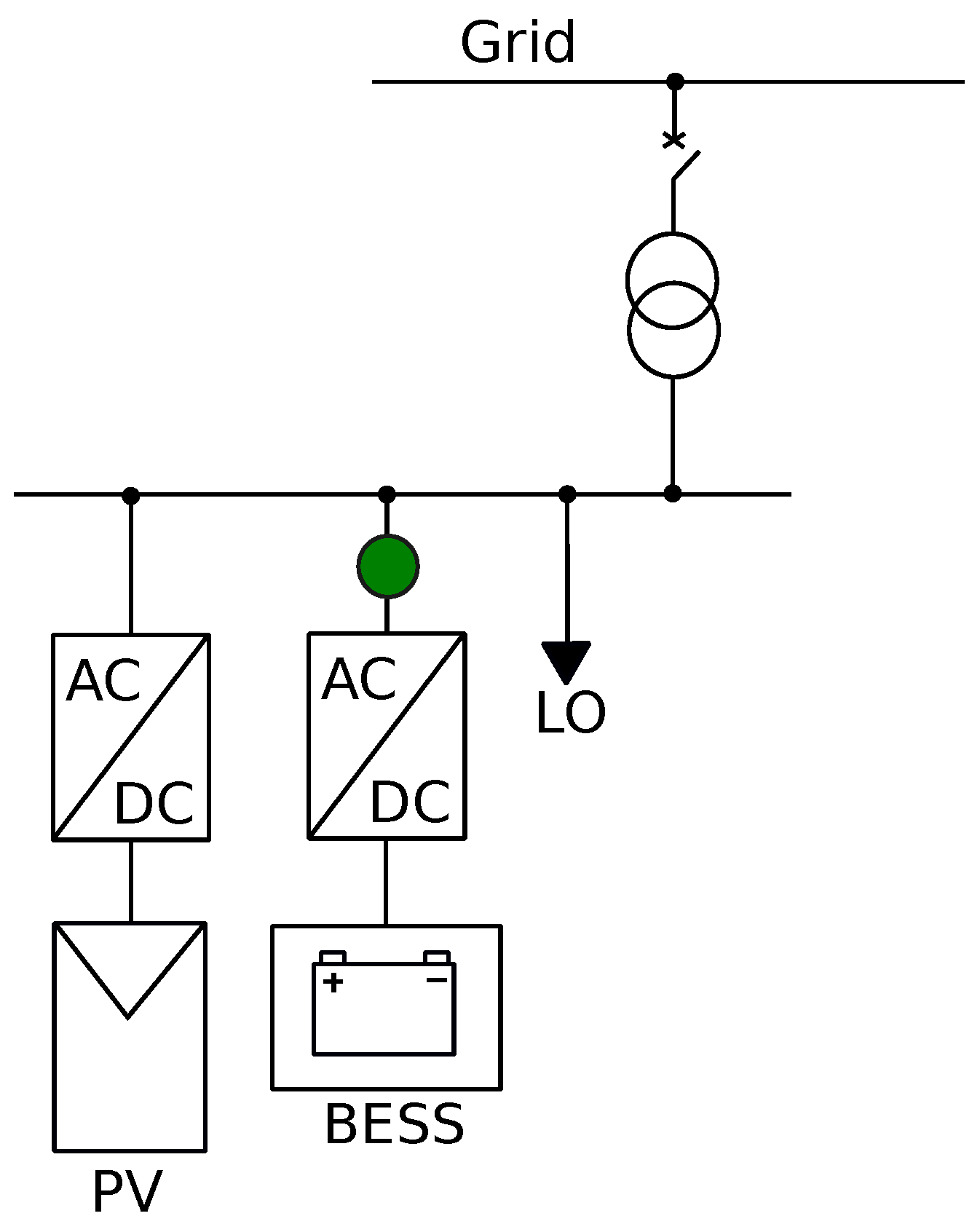
2.1. System Model

The system analyzed in this study comprises a power source, battery energy storage system, load, and electrical system. The point at which the power flow is crucial to assessing the reliability of the energy storage system is presented in Figure 1, indicated by a green circle.

The assessment of energy storage reliability in our study concerns generation reliability. In this case, it is similar to the assessment of the generation reliability of RESs, which depends mostly on weather conditions. The assessment is based on the simulation results.

2.2. BESS Control Strategy

The most important parameters of the BESS for simulation purposes are a minimal state of charge (SOC) and the following efficiencies: charging ${\eta }_{ch}$ and discharging ${\eta }_{dis}$ and auxiliary elements of system ${\eta }_s$, like power converters. Thus, the total efficiency is equal during charging and discharging:

$${\eta }_{ch-t}={\eta }_{ch}·{\eta }_s$$

(1)

$${\eta }_{dis-t}={\eta }_{dis}·{\eta }_s$$

(2)

The BESS control algorithm assumes that a consumer uses the produced energy for their own needs and that energy is charged to the BESS. If the BESS is full, the energy is returned to the power grid. In the case of energy shortage, energy is first drawn from the BESS, and if the SOC of the BESS is minimal, it is taken from the power grid.

Simulations are conducted with a one-hour step. The power balance $P_b$ in the system is calculated for every hour based on the production profile $P\left(t\right)$ and the consumption profile $D\left(t\right)$.

$$P_b\left(t\right)=P\left(t\right)-D\left(t\right).$$

(3)

Additionally, power excess $P_e\left(t\right)$ and power shortage $P_s\left(t\right)$ are calculated.

$$P_e\left(t\right)=\left\{\begin{array}{cc}{P}_b\left(t\right)\hfill & :P_b\left(t\right)>0\hfill \\ 0\hfill & :P_b\left(t\right)\le 0\hfill \end{array}\right.$$

(4)

$$P_s\left(t\right)=\left\{\begin{array}{cc}-P_b\left(t\right)\hfill & :P_b\left(t\right)<0\hfill \\ 0\hfill & :P_b\left(t\right)\ge 0.\hfill \end{array}\right.$$

(5)

If there is excess power $P_e\left(t\right)>0$ at hour t, then the BESS is charged with an energy equal to $E_{ch}\left(t\right)=1h·P_e\left(t\right)·{\eta }_{ch-t}$, including charging losses. If the BESS has not reached maximum capacity, then the state of charge increases by $E_{ch}\left(t\right)/Q$. If the maximum capacity is reached, the BESS’s state of charge remains at the $SO{C}_{max}$ level. Hence, in the next hour of simulation $t+1$, the state of charge of storage $SOC(t+1)$ is the following:

$$SOC(t+1)=min(SOC\left(t\right)+{\displaystyle \frac{P_{ch}\left(t\right)·{\eta }_{ch-t}}{Q}},SO{C}_{max}),$$

(6)

where Q is the the nominal capacity of energy storage [kWh], $P_{ch}\left(t\right)$ is the charge power [kW], and $SO{C}_{max}$ is the highest permissible level of charge.

If there is power shortage $P_s\left(t\right)>0$ at hour t, an attempt is made to draw power from the energy storage. The BESS is discharged with energy equal to $E_{dis}\left(t\right)=1h·P_e\left(t\right)·{\eta }_{dis-t}^{-1}$, including discharging losses. If the BESS has not reached the minimum capacity, then the state of charge is decreased by $E_{dis}\left(t\right)/Q$. If the minimum capacity is reached, the BESS’s state of charge remains at the $SO{C}_{min}$ level. Hence, in the next hour of simulation $t+1$, the storage state of charge $SOC(t+1)$ is as follows:

$$SOC(t+1)=max(SOC\left(t\right)-{\displaystyle \frac{P_{disch}\left(t\right)}{{\eta }_{dis-t}·Q}},SO{C}_{min}),$$

(7)

where Q is the nominal capacity of energy storage [kWh], $P_{disch}\left(t\right)$ is the discharge power [kW], and $SO{C}_{min}$ is the lowest permissible level of charge.

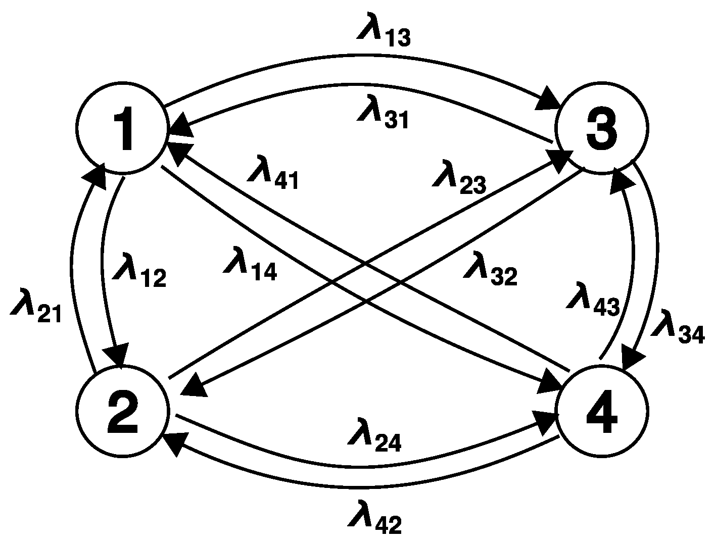
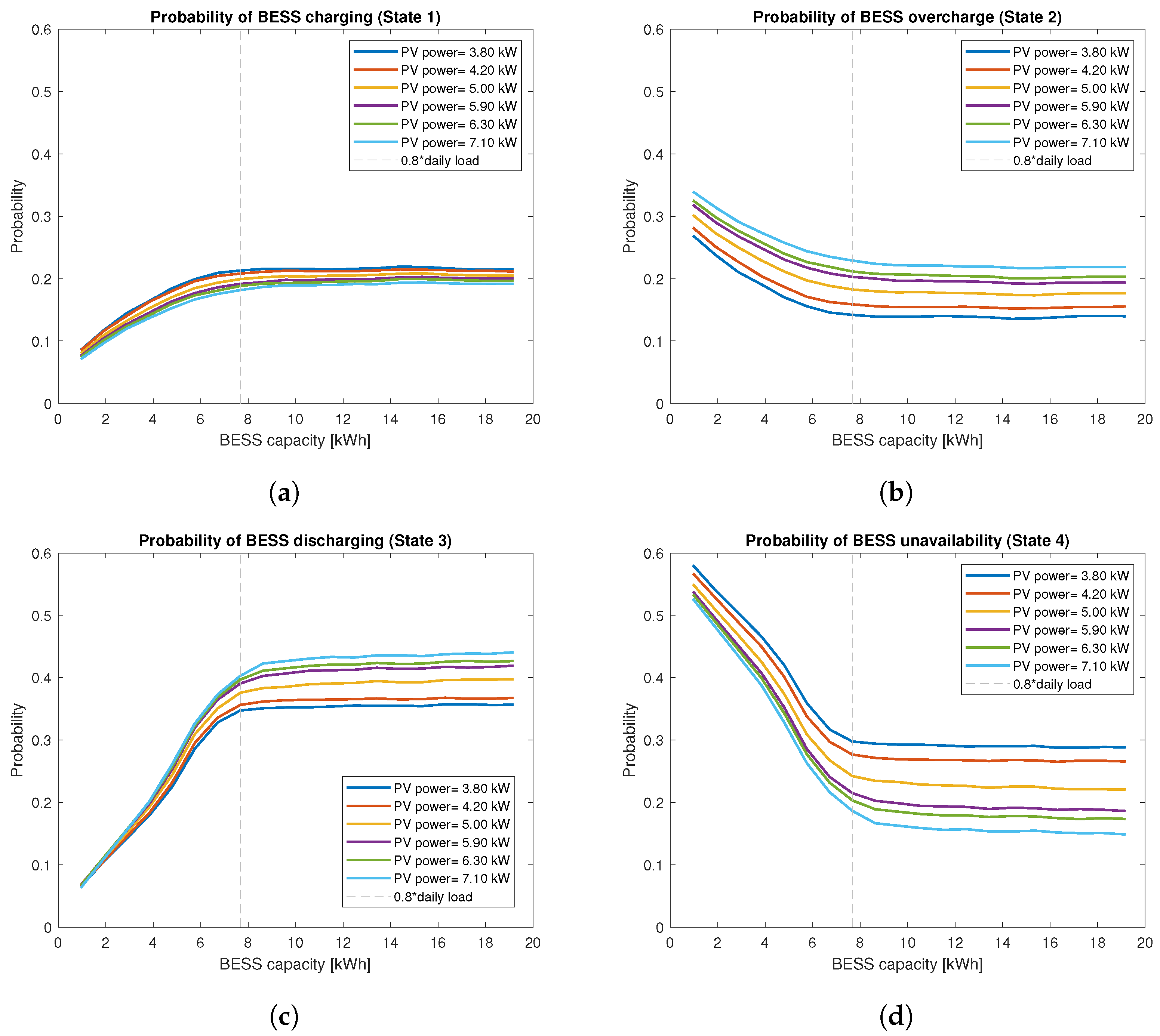
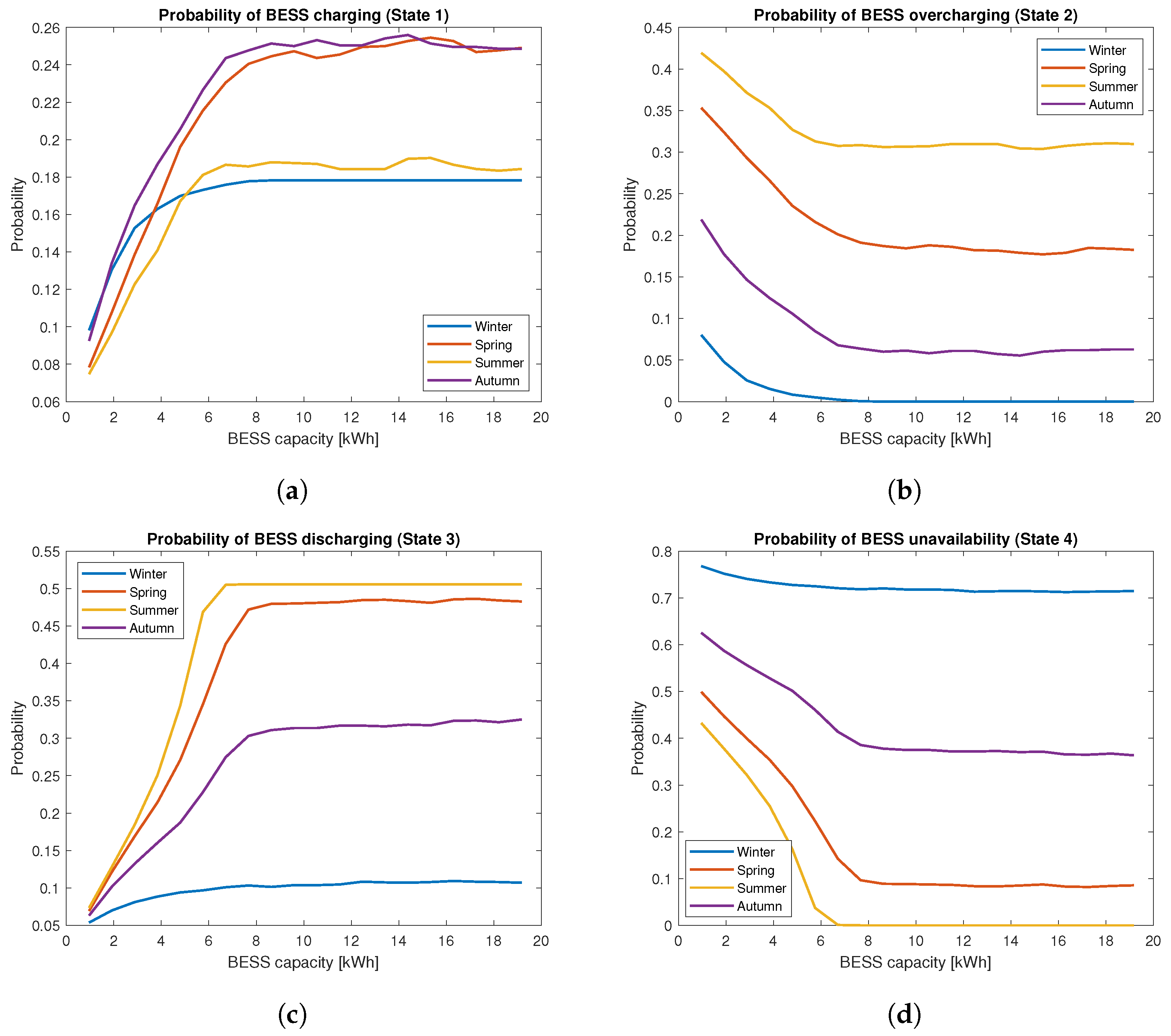
2.3. Reliability Model of BESS

During the simulations, the energy flow into and out of the BESS is analyzed as marked in Figure 1. Based on the analysis of a series of obtained hourly values of the power balance, it is assumed that at a given moment t, the BESS is in one of four states:

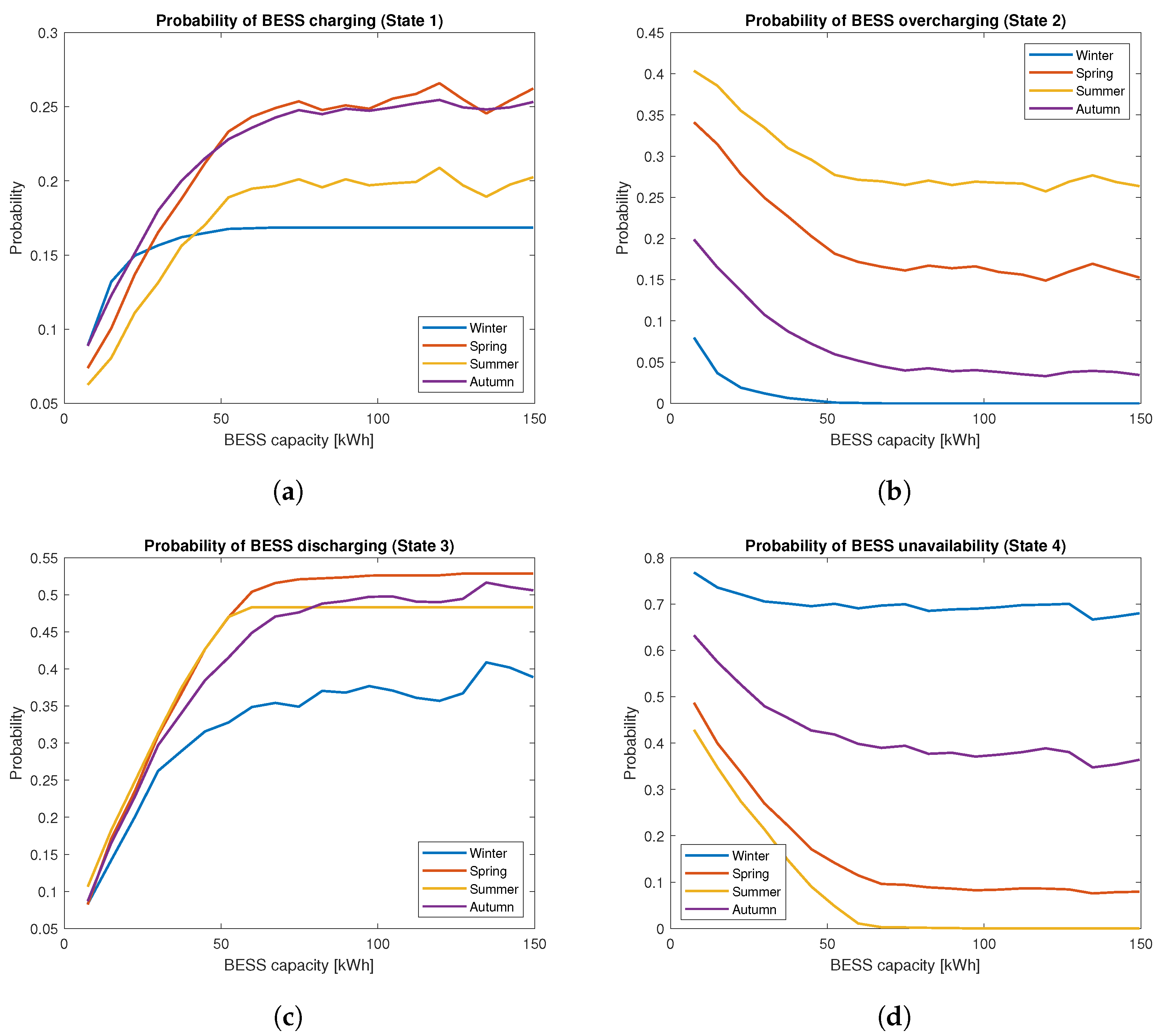
• State 1—there is excess power $P_e\left(t\right)>0$ in the system that the BESS can store ($SOC<SO{C}_{max}$);
• State 2—there is excess power $P_e\left(t\right)>0$ in the system, but the BESS is unable to store it (the $SOC$ has reached the maximum level $SO{C}_{max}$);
• State 3—there is a shortage of power in the system, $P_s\left(t\right)>0$, and the BESS can supply it ($SOC\ge SO{C}_{min}$);
• State 4—there is a shortage of power $P_s\left(t\right)>0$ in the system, but the BESS is unable to supply it (the $SOC$ has reached the minimum level $SO{C}_{min}$).

A graph of states of the analyzed system is shown in Figure 2, including possible transitions between states.

2.4. Determination of Reliability Parameters

The presented graph of BESS states is the base for determining the reliability model parameters of the analyzed system.

During a simulation, the state number is stored in the $State\left(t\right)$ vector. Based on the analysis of this series, the numbers of transitions between states $f_{i,j}$ are determined as follows:

$$f_{i,j}=card(\{t\in T)\wedge (t\ne 0):(State(t-1)=i)\wedge (State\left(t\right)=j)\}),$$

(8)

From the vector of states, the intensity of transitions from state i to state j is determined using the following formula:

$${\lambda }_{i,j}={\displaystyle \frac{f_{i,j}}{{\sum }_{k=1}^N{f}_{i,k}}},$$

(9)

where N is a number of states during a simulation.

The residence time $T_i$ in state i is determined based on the following equation:

$$T_i={\displaystyle \frac{1}{1-{\lambda }_{i,i}}}.$$

(10)

The stationary probabilities $p_i$ of being in state i are determined from the following relationship:

$$p_i={\displaystyle \frac{n_i}{{\sum }_{k=1}^N{n}_k}},$$

(11)

where $n_i$ is the number of occurrences of state i in the simulation results.

Another way to calculate the stationary probabilities is to use the set of Chapman–Kolmogorov equations which, for the proposed four-state model, take the following form:

$${\displaystyle \frac{d}{dt}}\mathbf{P}\left(\mathbf{t}\right)=\mathsf{\Lambda }\mathbf{P}\left(\mathbf{t}\right),$$

(12)

where $\mathbf{P}\left(\mathbf{t}\right)$ is the column vector of probabilities of being in particular states, and

$\mathsf{\Lambda }$ is the matrix of transition intensity,

$$\mathsf{\Lambda }=\left[\begin{array}{cccc}{\lambda }_{11}& {\lambda }_{21}& {\lambda }_{31}& {\lambda }_{41}\\ {\lambda }_{12}& {\lambda }_{22}& {\lambda }_{32}& {\lambda }_{42}\\ {\lambda }_{13}& {\lambda }_{23}& {\lambda }_{33}& {\lambda }_{43}\\ {\lambda }_{14}& {\lambda }_{24}& {\lambda }_{34}& {\lambda }_{44}\end{array}\right]$$

(13)

where

$$\begin{array}{c}{\lambda }_{11}=-({\lambda }_{12}+{\lambda }_{13}+{\lambda }_{14}),\\ {\lambda }_{22}=-({\lambda }_{21}+{\lambda }_{23}+{\lambda }_{24}),\\ {\lambda }_{33}=-({\lambda }_{31}+{\lambda }_{32}+{\lambda }_{34}),\\ {\lambda }_{44}=-({\lambda }_{41}+{\lambda }_{42}+{\lambda }_{43}).\end{array}$$

In order to obtain the stationary probabilities, Equation (12) is transformed into a system of linear equations:

$$\mathbf{0}=\mathsf{\Pi }\mathsf{\Lambda },$$

(14)

where $\mathsf{\Pi }$ is the column vector of stationary probabilities of states.

In order to eliminate the indeterminacy of the system Equation (14), it is completed with the following equation:

$$\sum _{i=1}^N{\mathsf{\Pi }}_{\mathbf{i}}=\mathbf{1}.$$

(15)

The system of equations for the analyzed four-state model is then described by

$$\left\{\begin{array}{c}0=p_1{\lambda }_{11}+p_2{\lambda }_{21}+p_3{\lambda }_{31}+p_4{\lambda }_{41}\hfill \\ 0=p_1{\lambda }_{12}+p_2{\lambda }_{22}+p_3{\lambda }_{32}+p_4{\lambda }_{42}\hfill \\ 0=p_1{\lambda }_{13}+p_2{\lambda }_{23}+p_3{\lambda }_{33}+p_4{\lambda }_{43}\hfill \\ 1=p_1+p_2+p_3+p_4\hfill \end{array}\right..$$

(16)

Using the method of determinants, one obtains

$$\left|D\right|=\left|\begin{array}{cccc}{\lambda }_{11}& {\lambda }_{21}& {\lambda }_{31}& {\lambda }_{41}\\ {\lambda }_{12}& {\lambda }_{22}& {\lambda }_{32}& {\lambda }_{42}\\ {\lambda }_{13}& {\lambda }_{23}& {\lambda }_{33}& {\lambda }_{43}\\ 1& 1& 1& 1\end{array}\right|$$

(17)

$$\begin{gathered} \left|D\right|={\lambda }_{11}({\lambda }_{22}({\lambda }_{33}-{\lambda }_{43})-{\lambda }_{32}({\lambda }_{23}-{\lambda }_{43})+{\lambda }_{42}({\lambda }_{23}-{\lambda }_{33})) \\ -{\lambda }_{21}({\lambda }_{12}({\lambda }_{33}-{\lambda }_{43})-{\lambda }_{32}({\lambda }_{13}-{\lambda }_{43})+{\lambda }_{42}({\lambda }_{13}-{\lambda }_{33})) \\ +{\lambda }_{31}({\lambda }_{12}({\lambda }_{23}-{\lambda }_{43})-{\lambda }_{22}({\lambda }_{13}-{\lambda }_{43})+{\lambda }_{42}({\lambda }_{13}-{\lambda }_{23})) \\ -{\lambda }_{41}({\lambda }_{12}({\lambda }_{23}-{\lambda }_{33})-{\lambda }_{22}({\lambda }_{13}-{\lambda }_{33})+{\lambda }_{32}({\lambda }_{13}-{\lambda }_{23})). \end{gathered}$$

$$|D_1|=\left|\begin{array}{cccc}0& {\lambda }_{21}& {\lambda }_{31}& {\lambda }_{41}\\ 0& {\lambda }_{22}& {\lambda }_{32}& {\lambda }_{42}\\ 0& {\lambda }_{23}& {\lambda }_{33}& {\lambda }_{43}\\ 1& 1& 1& 1\end{array}\right|$$

(18)

$$|D_1|={\lambda }_{31}({\lambda }_{22}{\lambda }_{43}-{\lambda }_{42}{\lambda }_{23})-{\lambda }_{21}({\lambda }_{32}{\lambda }_{43}-{\lambda }_{42}{\lambda }_{33})-{\lambda }_{41}({\lambda }_{22}{\lambda }_{33}-{\lambda }_{32}{\lambda }_{23}).$$

$$|D_2|=\left|\begin{array}{cccc}{\lambda }_{11}& 0& {\lambda }_{31}& {\lambda }_{41}\\ {\lambda }_{12}& 0& {\lambda }_{32}& {\lambda }_{42}\\ {\lambda }_{13}& 0& {\lambda }_{33}& {\lambda }_{43}\\ 1& 1& 1& 1\end{array}\right|$$

(19)

$$|D_2|={\lambda }_{11}({\lambda }_{32}{\lambda }_{43}-{\lambda }_{42}{\lambda }_{33})+{\lambda }_{31}({\lambda }_{42}{\lambda }_{13}-{\lambda }_{12}{\lambda }_{43})-{\lambda }_{41}({\lambda }_{32}{\lambda }_{13}-{\lambda }_{12}{\lambda }_{33}).$$

$$|D_3|=\left|\begin{array}{cccc}{\lambda }_{11}& {\lambda }_{21}& 0& {\lambda }_{41}\\ {\lambda }_{12}& {\lambda }_{22}& 0& {\lambda }_{42}\\ {\lambda }_{13}& {\lambda }_{23}& 0& {\lambda }_{43}\\ 1& 1& 1& 1\end{array}\right|$$

(20)

$$|D_3|={\lambda }_{11}({\lambda }_{42}{\lambda }_{23}-{\lambda }_{22}{\lambda }_{43})-{\lambda }_{21}({\lambda }_{42}{\lambda }_{13}-{\lambda }_{12}{\lambda }_{43})-{\lambda }_{41}({\lambda }_{12}{\lambda }_{23}-{\lambda }_{22}{\lambda }_{13}).$$

Then:

$$p_1={\displaystyle \frac{|D_1|}{\left|D\right|}},p_2={\displaystyle \frac{|D_2|}{\left|D\right|}},p_3={\displaystyle \frac{|D_3|}{\left|D\right|}}$$

(21)

Similarly, the determinant $|D_4|$ and the stationary probability $p_4$ can be determined, but it is simpler to calculate it from the relation $p_4=1-p_1-p_2-p_3$.

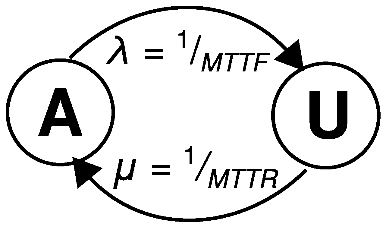
2.5. Simplified Two-State Model

The reliability model proposed in our research has four states. However, the most important information regarding reliability is the ability or inability to perform a required function. Therefore, the current model can be transformed into a new two-state model in which the first state represents availability (A) and the second state represents unavailability (U). To modify the proposed four-state model, it would be necessary to assign the first three states State 1 (charging), State 2 (overcharging), and State 3 (discharging) to the state of availability (A) and the current State 4 (discharging when $SOC=SO{C}_{min}$) to the state of unavailability (U). Figure 3 presents a graph of a two-state model. Such a simplified model can be used to represent energy storage in power system reliability analyses more readily.

The stationary probabilities of availability p and unavailability q are determined by the following equations:

$$p={\displaystyle \frac{\mu }{\mu +\lambda }},q={\displaystyle \frac{\lambda }{\mu +\lambda }}.$$

(22)

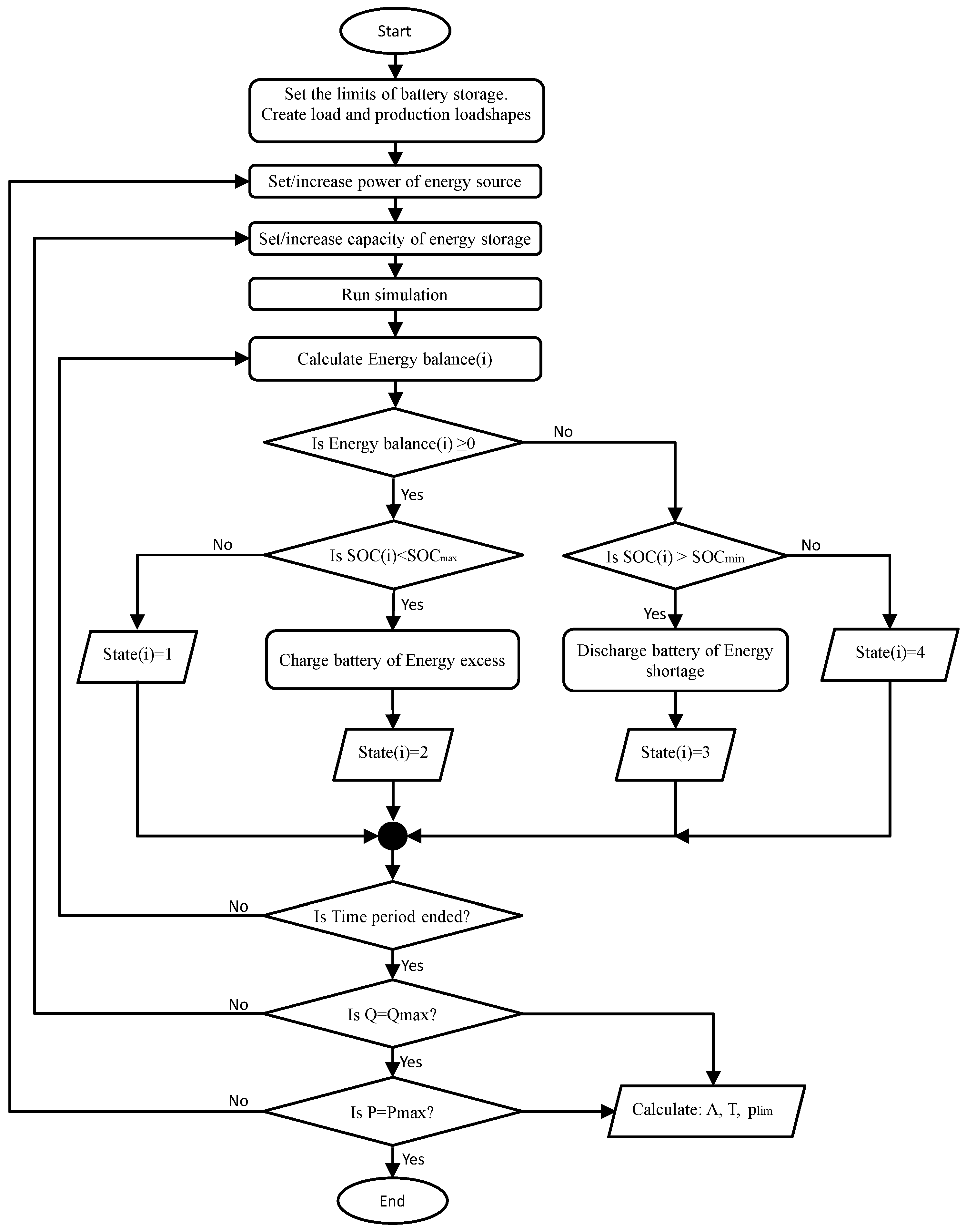
2.6. Simulation Algorithm

To assess the BESS reliability, multiple simulations are carried out, including different capacities, the power of photovoltaics, and two kinds of load profiles: households and public office buildings. For every energy consumer, we first determine its load profile and, further, we add a PV power source. The initial value of the photovoltaic power P is selected so that annual production equals an end user’s annual electricity demand, which is a typical approach in scaling PV systems. In subsequent iterations, the initial power is increased successively by 20% up to twice the initial value. For each PV power, simulations are performed for a series of values of energy storage capacity Q. The initial nominal BESS capacity is equal to 10% of the value of the average daily energy demand and is successively increased by 10% until it reaches 200%. It is assumed that the maximal power of the BESS is equal half of its capacity. The proposed approach makes it possible to fit PV and BESS capacity values to the specific end user by relating the values to a nominal load. Therefore, this methodology is versatile and can be used for any type of load. Figure 4 presents the algorithm for the simulations.

3. Results and Discussion

Poland is an example of a country in which there are public subsidies for hybrid PV-ESS installations; in addition, the net-metering system was recently replaced by net billing there. Energy sale prices for newly built installations are settled according to hourly rates on the day-ahead market of the Polish Power Exchange, while purchase prices are set according to the energy seller’s tariff [37]. Such a system makes it more advantageous for prosumers to integrate RES installations with an energy storage facility that enables the storage of surplus energy than to sell it, often at rates, to DSO. Thus, from the Polish perspective, a significant increase in the number of residential BESS installations cooperating with photovoltaic systems is expected in the coming months and years. Therefore, we present a case study based on conditions specific to Poland. The simulations were performed in Matlab 2022a, including parameter calculations and modeling the power source, load profiles, and BESS.

3.1. PV Model

PV output power is based on average one-hour solar data defined for 35° module inclination and south orientation (azimuth 0°) for the central region of Poland collected in the 2016–2020 period and taken from the PV Geographical Information System [38].

The PV output power may be described by the following equation [35,39]:

$$P_{PV}\left(t\right)=N_{PV}{\displaystyle \frac{G_{irr}\left(t\right)}{1000}}{\eta }_c{\eta }_{s-PV}·S_{PV}$$

(23)

where $N_{PV}$ is the number of modules, $G_{irr}$ is the global horizontal irradiance scaled to a slope [kW/m²], $S_{PV}$ is the surface of a module, ${\eta }_{s-PV}$ is the system efficiency, and ${\eta }_c$ is the module efficiency, including the temperature correction factor determined via Equation (24) [40],

$${\eta }_c={\eta }_{ref}[1-{\beta }_{ref}(T_c\left(t\right)-T_{ref})]$$

(24)

where the reference values ref are given in a product’s data sheet and are usually defined in STC and $T_c$ is the module temperature, which may be calculated using Equation (25) [35],

$$T_c\left(t\right)=T_a\left(t\right)+G_{irr}\left(t\right)\left(\frac{NOCT-20}{0.8}\right)$$

(25)

where $T_a$ is the ambient temperature and $NOCT$ is the normal operating temperature of a module.

In the simulations, we used a PV module, the parameters of which are presented in

Table 1. PV module parameters.

Power	Module Efficiency	Surface	System Efficiency
P	${\eta }_{PV}$	S	${\eta }_{system}$
[W]	[%]	[m2]	[%]
420	21.4	1.953	88

[41].

3.2. Load Model

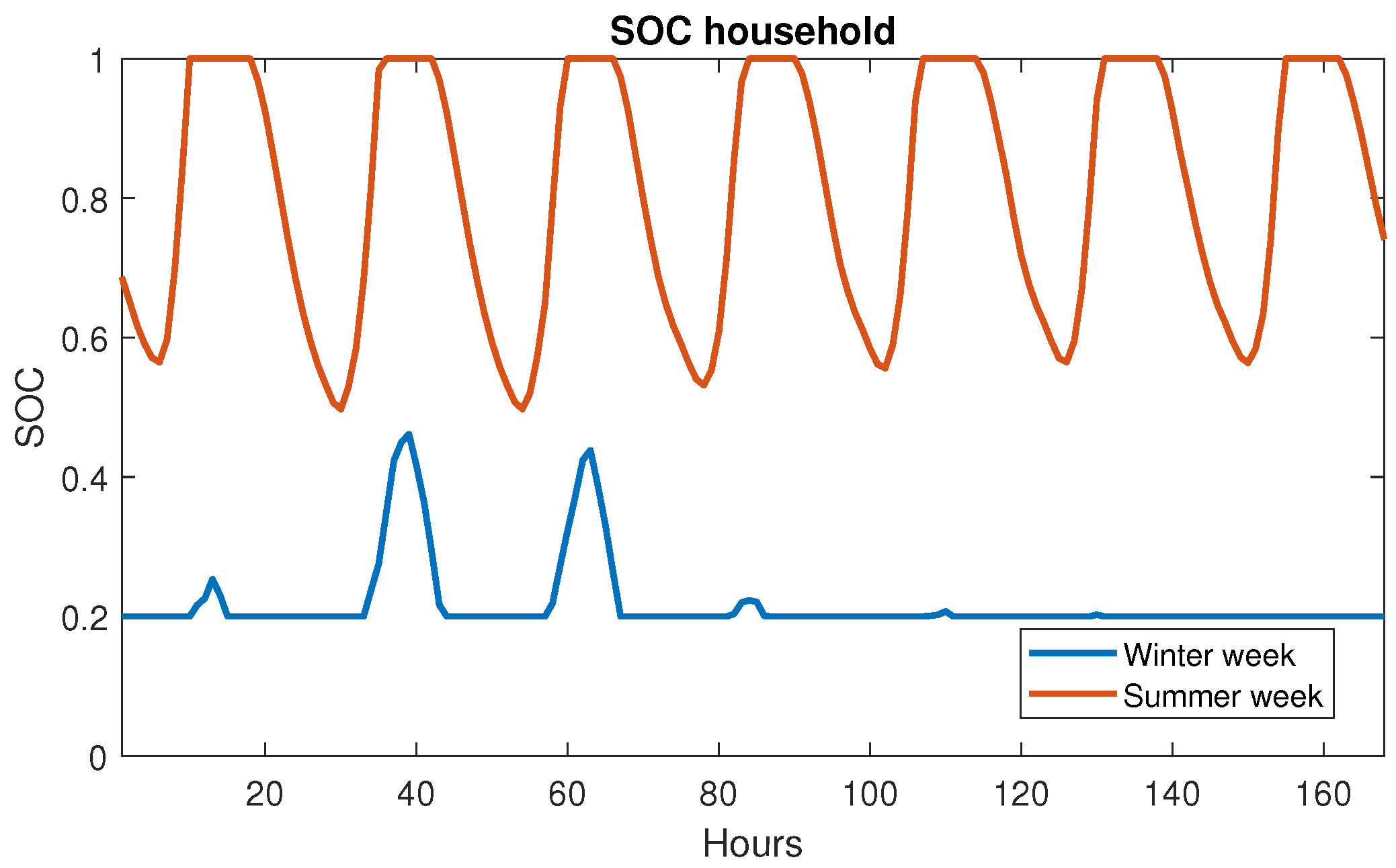
3.2.1. Residential Profile

A residential load profile is based on a standard profile prepared by a Polish Distributed System Operators [42]. A profile is constructed at a one-hour step and scaled for an end user whose yearly energy consumption is equal to 3500 kWh. Figure 5 presents a household profile for an exemplary week during winter and summer each.

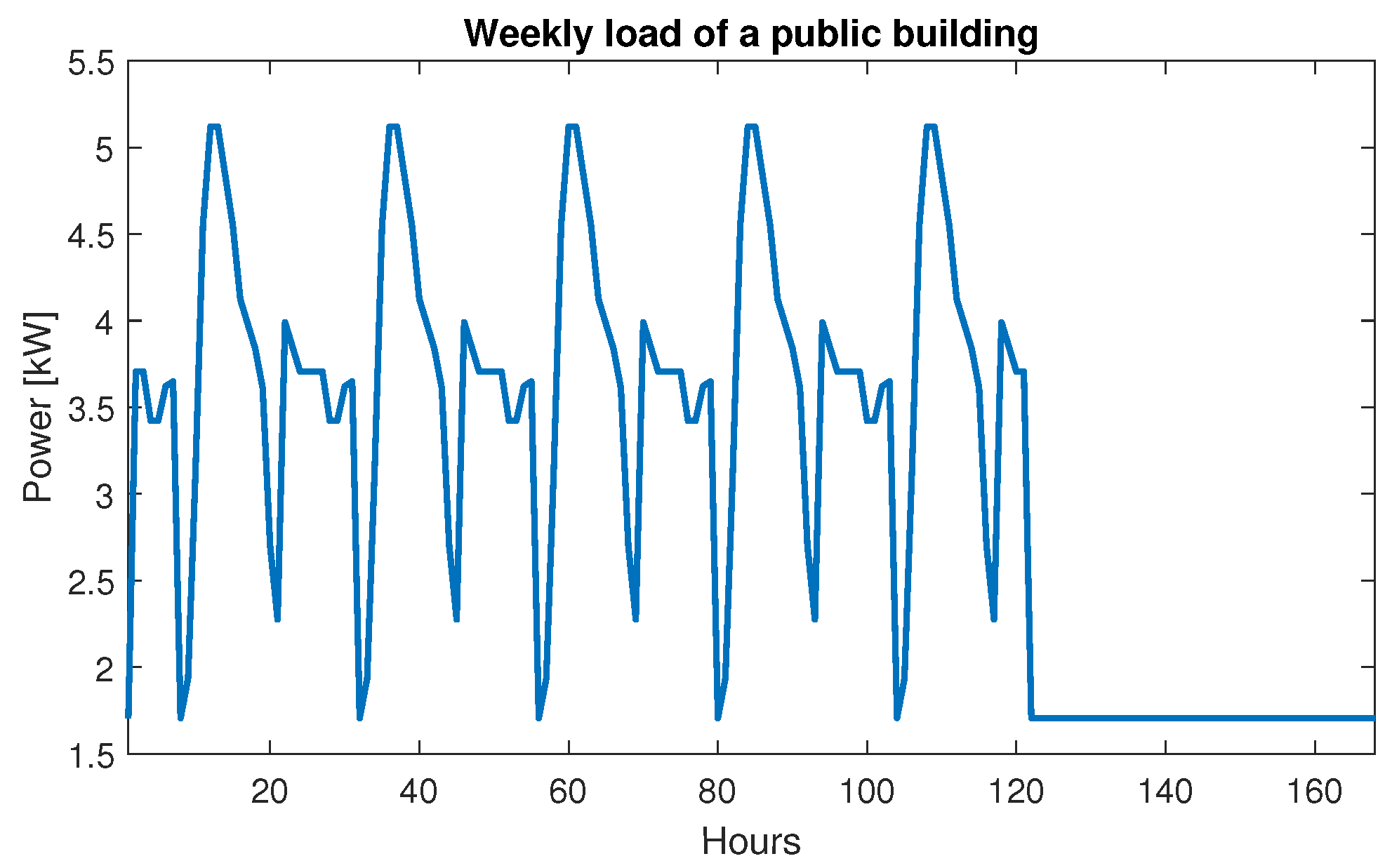
3.2.2. Public Office Profile

A public office load profile is characterized by fixed working hours from Monday to Friday, usually 8–16, and free weekends. The shape of the profile is based on statistics data presented in [43] and scaled to real data obtained from a public office localized in the central region of Poland, the yearly demand of which is estimated at a value of 27,000 kWh. Furthermore, due to the implementation of European directives regarding the promotion of electric cars, it is assumed that the office has an electric car for its own use. An electric car charges only during workdays between 8 p.m. and 6 a.m. A weekly profile is presented in Figure 6.

3.3. Battery Energy Storage Model

It is assumed that the energy storage model corresponds to a lithium-ion battery, which enables quick charging and discharging without deterioration of its lifetime and useful capacity. Based on battery manufacturer data, the recommended power is usually equal in value to half the battery’s capacity. Therefore, the simulations assume that the BESS can be charged and discharged at a maximum power equal to half its capacity, which we call $P_{max-BESS}$.

Based on the data and our own experience, the minimal state of charge of the battery is assumed to be 20%, while the maximal state of charge is equal to 100%. The efficiency during both charging ${\eta }_{ch}$ and discharging ${\eta }_{dis}$ is 94%. The efficiency of the system ${\eta }_s$ is assumed at the level of 94% [44]. This yields an overall efficiency equal to 88% for both charging and discharging. The self-discharge rate in the simulations is not included as the operating time between cycles is very short, making this rate negligible.

3.4. Residential Installation

Several PV and BESS capacity values were simulated in accordance with Section 2.6. The simulations start with a PV size equal to 3.8 kW, production for which covers annual energy consumption and is successively increased by 20% until 7.2 kW. The BESS capacity for PV power is increased from 0.96 kWh to 19.15 kWh with a step of about 1 kWh. The capacity of 9.58 kWh corresponds to the average daily consumption.

Figure 7 presents the energy flow into (positive) or out of (negative) the BESS for a residential installation during an exemplary week in winter (January) and summer (July). The figure presents the results for the initial PV power and capacity values of the BESS equal to the average daily energy consumption. Figure 8 shows a state of charge under the same conditions.

It is clearly visible that during winter, the amount of excess energy is very low and not sufficient to fully charge the BESS. For the vast majority of time, the charge level is equal to the minimum permissible value. During summer, the amount of excess energy is higher and sufficient to fully charge the BESS. For the curves in the figures, the daily trend of charging and discharging to and from storage related to energy generation and consumption is visible.

Table 2. Residence time in specific states for residential installation and PV power 4.2 kW.

${\mathbf{Q}}_{\mathbf{nom}}$	${\mathbf{T}}_1$	${\mathbf{T}}_2$	${\mathbf{T}}_3$	${\mathbf{T}}_4$	${\mathbf{p}}_1$	${\mathbf{p}}_2$	${\mathbf{p}}_3$	${\mathbf{p}}_4$
kWh	h	h	h	h	-	-	-	-
0.96	2.03	7.80	1.63	13.96	0.086	0.269	0.065	0.580
1.92	2.75	7.65	2.64	13.02	0.117	0.238	0.106	0.540
2.87	3.40	7.28	3.60	12.07	0.145	0.210	0.142	0.503
3.83	3.85	7.15	4.49	11.28	0.164	0.191	0.179	0.466
4.79	4.34	6.78	5.68	10.15	0.185	0.170	0.225	0.420
5.75	4.68	6.53	7.24	10.59	0.199	0.156	0.286	0.359
6.71	4.91	6.35	8.30	12.23	0.209	0.146	0.328	0.317
7.66	5.00	6.37	8.79	14.65	0.213	0.142	0.347	0.298
8.62	5.06	6.46	8.86	15.34	0.216	0.139	0.351	0.294
9.58	5.07	6.48	8.97	15.64	0.216	0.139	0.352	0.293
10.54	5.06	6.46	8.97	15.72	0.216	0.139	0.353	0.293
11.50	5.04	6.46	8.98	15.66	0.215	0.140	0.354	0.291
12.45	5.07	6.59	9.07	15.67	0.216	0.139	0.355	0.290
13.41	5.09	6.51	9.14	15.69	0.217	0.138	0.355	0.290
14.37	5.15	6.46	9.12	15.69	0.219	0.136	0.355	0.290
15.33	5.14	6.45	9.13	15.52	0.219	0.136	0.354	0.291
16.29	5.09	6.54	9.18	15.75	0.217	0.138	0.357	0.288
17.24	5.05	6.56	9.26	15.84	0.215	0.140	0.358	0.288
18.20	5.04	6.64	9.29	15.71	0.215	0.140	0.356	0.289
19.16	5.05	6.65	9.29	15.70	0.215	0.140	0.357	0.288

presents the results of residence time T in particular states. The results are obtained for a PV power equal to the basic value, which is 3.80 kW. Based on residence time values, it is possible to draw a completed four-state graph and calculate stationary probabilities based on Chapman–Kolmogorov equations.

Then, based on reliability calculations (such as the transitions between states and the duration of them) we assess the probability of four states of the BESS: State 1—charging; State 2—overcharge (SOC = ${\mathrm{SOC}}_{max}$); State 3—discharging; and State 4—BESS unavailability (SOC ≤ ${\mathrm{SOC}}_{min}$). From the perspective of reliability, the most relevant is State 4, when there is energy demand in the prosumer installation but there is no available energy in the BESS. The probabilities of the other states may offer some additional information. Figure 9 presents the probabilities of every state for variable PV power and battery capacity.

In Figure 9, it may be seen that for a BESS capacity over about 8 kWh, which is 80% of an average daily load, there is no significant change in the probability value for every state. In particular, it is worth looking at Figure 9d, which shows the probability of State 4. From this, it can be concluded that for a constant PV source power, increasing the BESS capacity does not clearly improve its availability. However, it may lead to an increase in capital expenditure and maintenance costs. The graph also shows that the highest PV power occurs with the lowest probability of State 4. The probability in this state stabilizes depending on the PV power ranging from about 0.14 to 0.3. Analyzing Figure 9 of State 1, the divergence between the results for different PV power values is the smallest. The probability of State 1 slightly grows in the function of the BESS capacity and is established at about 0.2. Figure 9b shows that increasing the PV power increases the probability of overcharge. Obviously, higher PV power results in more excess energy and thus a higher probability that the storage system will be fully charged. The highest PV power results in a stable probability of about 0.22, while the lowest power leads to a nearly constant probability of about 0.13. Similarly, Figure 9c presents that higher PV power causes higher probability of State 3—discharging. In this state, the established probability deviates from 0.36 for the highest power to 0.44 for the lowest PV power.

PV generation in Polish weather conditions is characterized by high variability. There is a significant difference between the number of hours of sunshine in each season. For this reason, a more detailed model was made with distinction between seasons. Figure 10 presents the results of the probability of each state for a PV power equal to 3.8 kW. Looking at Figure 10, it can be seen that, again, the probability values become roughly constant for a BESS capacity equal to about 80% of the average daily demand. From Figure 10a it can be observed that the probability of State 1 (charging) is the lowest in winter, which can be explained by low energy generation from PV installations. Successively, higher values occur in summer, which, in turn, is associated with high PV and rapid attainment of the maximum state of charge. This trend is clearly visible in Figure 10b. The probability of overcharging is the highest in summer, followed by spring, while it is minimal in winter. Analyzing Figure 10c, it can be seen that the probability of State 3 (discharge) is quite high and similar for spring and summer, followed by autumn, while the lowest value occurs in winter. The most significant results are shown in Figure 10d for State 4 (unavailable BESS). In this case, it is clear that a very high probability occurs in winter and is hardly independent of the battery capacity. Lower values of probability occur in autumn and spring. On the other hand, State 4 does not occur at all in summer, even with an increase in capacity. In this context, it is worth noting that in order to ensure a higher reliability in winter for a system built from a PV source and energy storage, increasing the capacity of the battery does not achieve the desired result but increases costs. The solution should therefore be found in a different manner.

3.5. Public Office Building

Simulations for a public office building are carried out by taking an office load profile and various configurations of PV power and capacity into account. The PV power basic value is equal to 27.3 kW and increases by about 20% until the power equals 54.6 kW, which doubles the initial value. The BESS capacity starts from a value of 7.4 kWh and equals 10% of an average daily load. It successively rises by about 10% until it reaches almost 150 kWh, which is 200% of an average daily load. The simulations are carried out in accordance with the algorithm in Section 2.6. The efficiencies and the BESS’s minimal state of charge are the same as for the residential installation.

Figure 11 presents the energy flow into (positive) or out of (negative) the BESS for an office installation for, the same as above, winter and summer weeks. The figure shows the results for the initial PV power, and the BESS capacity equals a daily load. During a summer week, there are surpluses of energy that flow into the BESS. Thanks to this, energy may be taken out from the BESS when needed. The daily cycle of operation is clearly visible here. The winter week curve is the opposite. Energy surpluses are small and insufficient to meet the energy demand for an extended period of time. This regularity is confirmed by the graphs in Figure 12, which present the SOC under the same conditions. During summer, the state of charge is high and often does not reach a minimum state. In contrast, during winter, the state of charge rises only slightly, and the excess energy is not sufficient to fully charge the BESS.

Then, exactly as for the household, we ran simulations and calculated transitions between states, the duration of each state, and stationary probabilities. Figure 13 shows the probabilities of each state for different BESS capacity and PV power values.

It is worth noting that the energy demand profile of the public office building largely coincides with the energy generation profile. Despite this, the results obtained for this consumer (Figure 13) are not significantly better compared to a residential building, when peaks in energy demand occur at other hours of the day. The shapes of the curves are similar and allow one to determine the limit of the BESS capacity when the values of probabilities hardly change. The BESS capacity per this limit is, again, equal to about 80% of the average daily energy demand. Figure 13a shows that the probability of State 1 (charging) is hardly invariant and equal to about 0.2. This value is independent of the PV power. Figure 13b presents the probability of State 2 (overcharged). Its value equals 0.21 for the highest PV power and 0.11 for the lowest PV power. Figure 13c presents the probability of State 3 (discharging). For the highest PV power, the probability stabilizes for a value of about 0.48, and for the lowest, for a value of about 0.37. The probability of State 4, BESS unavailability, is presented in Figure 13d. The results show that the highest PV power results in the lowest established probability of about 0.13. The lowest PV power, in turn, results in an established probability of about 0.3. It can also be seen in the graphic that increasing the BESS capacity beyond a certain value does not improve its reliability.

Figure 14 shows the probability values for each state by season. Figure 14a presents the probability of State 1. It may be seen that for an established probability (for about 60 kWh of the BESS capacity), the highest values are found for spring and autumn, while the lowest are found for winter. In comparison, in Figure 14b, it may be observed that the highest probability of overcharging occurs in summer, followed by spring, autumn, and winter. Figure 14c shows that the probability of State 3, discharging, is the highest in summer and spring and lower in autumn and winter. Figure 14d shows the probability of State 4, BESS unavailability. Here, the highest probability occurs in winter and is approximately 70%, followed by autumn, when it is about 40%, and it is lower in spring—below 10%—and 0% in summer.

Figure 14 shows a high probability divergence of each state dependent on season. What is worth noting that the winter is the worst, considering unavailability, independent of the BESS capacity. Some positive effects may cause a PV power increase; however, at the same time, this causes higher costs, and the BESS availability increases only slightly. Thus, it is not a good practice to optimize BESS size based on winter conditions.

Table 3. Residence time in specific states for office building installation and PV power of 27.3 kW.

${\mathbf{Q}}_{\mathbf{nom}}$	${\mathbf{T}}_1$	${\mathbf{T}}_2$	${\mathbf{T}}_3$	${\mathbf{T}}_4$	${\mathbf{p}}_1$	${\mathbf{p}}_2$	${\mathbf{p}}_3$	${\mathbf{p}}_4$
kWh	h	h	h	h	-	-	-	-
7.48	1.90	7.81	2.24	14.38	0.078	0.257	0.087	0.578
14.96	2.63	7.63	3.91	12.77	0.109	0.226	0.152	0.513
22.43	3.31	7.18	5.20	11.52	0.137	0.198	0.202	0.463
29.91	3.81	6.96	6.43	11.20	0.158	0.177	0.249	0.416
37.39	4.25	6.62	7.37	10.61	0.177	0.159	0.286	0.379
44.87	4.59	6.34	8.29	10.84	0.191	0.145	0.321	0.344
52.35	4.91	6.12	8.78	10.86	0.205	0.131	0.340	0.325
59.82	5.05	6.17	9.39	12.81	0.211	0.125	0.363	0.301
67.30	5.15	6.09	9.64	15.14	0.214	0.121	0.371	0.294
74.78	5.23	6.05	9.61	15.30	0.218	0.117	0.370	0.295
82.26	5.15	6.16	9.85	15.54	0.214	0.121	0.379	0.286
89.74	5.22	6.11	9.87	15.77	0.217	0.118	0.379	0.286
97.21	5.17	6.21	9.97	16.22	0.216	0.120	0.381	0.283
104.69	5.24	6.11	9.91	16.35	0.218	0.117	0.379	0.286
112.17	5.28	6.09	9.83	16.42	0.220	0.115	0.376	0.289
119.65	5.39	5.94	9.83	16.44	0.225	0.111	0.374	0.291
127.13	5.22	6.17	9.95	16.64	0.218	0.118	0.376	0.289
134.60	5.11	6.38	10.41	17.02	0.213	0.122	0.395	0.270
142.08	5.22	6.21	10.28	16.54	0.218	0.118	0.391	0.274
149.56	5.32	6.10	10.22	16.26	0.223	0.113	0.386	0.278

shows residence time results in each state for office building installations and corresponding probabilities for a basic scenario of a 27.3 kW PV installation. Based on these results, it is possible to prepare a completed four-state graph and, with the use of Chapman–Kolmogorov equations, calculate boundary probabilities.

3.6. Two-State Model

A modification of the four-state model into a two-state model yielded results in the form of the probability of a state of availability, $P_{av}$, or a state of unavailability, $P_{unav}$. The residence time in each state can be defined as MTTF—the mean time to failure—and MTTR—the mean time to repair. The failure rate $\lambda$ is equal to 1/MTTF and the repair rate $\mu$ is equal to 1/MTTR. The probability of the availability state can be determined from the four-state model as the sum of States 1, 2 and 3, and the probability of unavailability is equal to the probability of State 4. Another way to calculate the probability of availability is to use the following formula, ${\displaystyle \frac{\mu }{\mu +\lambda }}$, and to calculate the probability of unavailability using formula ${\displaystyle \frac{\lambda }{\mu +\lambda }}$.

The results of MTTF and MTTR for selected PV power variants for a residential installation are presented in

Table 4. MTTF and MTTR for residential installation.

	P = 3.78 kW		P = 4.20 kW		P = 5.04 kW
${\mathbf{Q}}_{\mathbf{nom}}$	MTTF	MTTR	MTTF	MTTR	MTTF	MTTR
[kWh]	[h]	[h]	[h]	[h]	[h]	[h]
0.96	10.13	13.96	10.36	13.53	10.69	13.02
1.92	11.14	13.02	11.25	12.52	11.67	12.03
2.87	11.96	12.07	12.21	11.63	12.64	11.07
3.83	12.95	11.28	13.16	10.74	13.67	10.11
4.79	14.02	10.15	14.32	9.59	14.97	8.93
5.75	18.96	10.59	19.59	9.96	20.87	9.30
6.71	26.47	12.23	26.88	11.32	28.26	10.28
7.66	34.76	14.65	35.39	13.47	38.82	12.33
8.62	37.02	15.34	39.40	14.58	43.25	13.18
9.58	38.00	15.64	39.76	14.56	44.21	13.33
10.54	38.25	15.72	40.30	14.70	47.24	13.91
11.50	38.31	15.66	40.31	14.68	47.65	13.93
12.45	38.64	15.67	40.35	14.65	48.39	14.07
13.41	38.62	15.69	39.91	14.41	49.29	14.08
14.37	38.62	15.69	40.08	14.58	47.77	13.81
15.33	38.12	15.52	40.10	14.55	47.45	13.70
16.29	39.24	15.75	40.48	14.52	49.75	14.08
17.24	39.49	15.84	40.38	14.62	49.79	14.04
18.20	38.93	15.71	40.39	14.61	50.54	14.24
19.16	38.95	15.70	40.45	14.54	50.94	14.32

, while for an office building installation, they are presented in

Table 5. MTTF and MTTR for office building installation.

	P = 27.30 kW		P = 32.76 kW		P = 38.22 kW
${\mathbf{Q}}_{\mathbf{nom}}$	MTTF	MTTR	MTTF	MTTR	MTTF	MTTR
[kWh]	[h]	[h]	[h]	[h]	[h]	[h]
7.48	10.54	14.38	10.69	13.20	10.86	12.53
14.96	12.15	12.77	12.34	11.56	12.58	10.81
22.43	13.40	11.52	13.62	10.29	13.84	9.55
29.91	15.80	11.20	16.09	9.80	16.46	8.91
37.39	17.43	10.61	18.17	9.26	18.70	8.31
44.87	20.74	10.84	21.37	9.22	22.10	8.08
52.35	22.66	10.86	23.67	9.10	25.72	8.20
59.82	29.85	12.81	33.73	11.36	36.65	10.14
67.30	36.60	15.14	40.83	13.15	43.55	11.46
74.78	36.75	15.30	41.77	13.58	45.87	12.06
82.26	39.11	15.54	44.85	13.84	50.44	12.49
89.74	39.57	15.77	44.38	13.92	49.94	12.53
97.21	41.30	16.22	45.79	14.10	51.65	12.66
104.69	41.17	16.35	44.39	13.91	51.18	12.66
112.17	40.72	16.42	43.04	13.75	50.17	12.75
119.65	40.33	16.44	43.18	13.97	49.31	12.72
127.13	41.25	16.64	44.01	13.90	51.73	13.05
134.60	46.33	17.02	48.30	13.73	57.63	12.90
142.08	44.17	16.54	47.36	13.80	56.86	13.10
149.56	42.42	16.26	46.10	13.80	55.29	13.04

.

Compared to other works [34,35] related to an end-user perspective of BESS reliability, the model proposed in this paper provides a different perspective and results. Ref. [34] deals with the reliability analysis of a low-voltage feeder considering distributed energy sources integrated with storage (DES) behind the meter. The analysis provides a comprehensive investigation of sensitivity factors, such as climate zone, power source size, and load profile, to assess the impact of DES on feeder reliability. The storage model, as in this study, includes parameters such as the SOC, the capacity, and the power, and the power balance of the prosumer installation is included in the calculation of reliability indicators. Ref. [35] addresses the issue of improving the reliability of residential customers by applying hybrid energy resources and ESSs and analyses the impact of their different sizes and configurations.

In contrast, our work focused on the battery storage model at its core, assessing the generation reliability based on an energy balance in prosumer installations. This study also investigated how the storage capacity and PV size can affect the probability of storage unavailability and the ratio of energy self-consumption in an end-user installation. Two groups of customers were analyzed in our study—households and offices. The BESS integration scenario assumed maximum self-consumption. Based on the results, it can be concluded that for both groups, sufficient BESS capacity represents approximately 80% of the average daily energy consumption. This level was obtained independently of the PV capacity. However, an increase in a PV power can reduce the probability of battery unavailability by almost two times. In this case, more of the surplus energy is supplied to the grid, which may not be cost-effective and does not cover the capital expenditure incurred for the installation.

The paper also analysed the impact of weather conditions and load profile on the results. Figure 15 shows a comparison of BESS unavailability between residential and public office buildings depending on season. The graph refers to a basic PV capacity for both consumers. It may be seen that there are no significant differences between the results.

The presented approach enables an examination of the BESS reliability problem from the perspective of an end user whose primary objective is to optimize the operation of domestic installation and minimize electricity costs.

4. Conclusions

This study proposes a new four-state model to evaluate the generation reliability of a battery energy storage system cooperating with a PV source. This research deals with small-scale PV installations dedicated to residential and public consumers, which is especially needed at present, when an energy transition based on a citizen involvement is developing. The reliability of a BESS is evaluated using an integration scenario that assumes that all surplus energy is first stored in the battery, and in case of an energy shortage, it is first drawn from it. The proposed methodology is similar to the one used for the reliability assessment of renewable energy sources such as wind turbines and photovoltaics.

The BESS reliability model proposed in our research can be simplified to a two-state model which provides information on the reliability and unreliability states of the storage system, which is crucial information for end users. One of the most important conclusions from our research is the BESS capacity limit, above which the probability of BESS unreliability does not increase significantly. For both public and domestic consumers, this limit is approximately 80% of the average daily energy consumption. For an average household with an annual energy consumption of 3500 kWh, a BESS capacity of approximately 7.7 kWh is sufficient. For an office with an annual energy consumption of 27,000 kWh, a storage capacity of approximately 60 kWh should be adequate. This information can be very helpful in choosing an energy storage size without oversizing and incurring excess costs. The results are credible for an integration scenario assuming maximum auto-consumption; however, the model should be modified if other scenarios are investigated. Moreover, the results show that the probability of a particular state strongly depends on weather conditions, though calculations are carried out for a temperate climate zone. For a residential prosumer with a fixed PV capacity, the unavailability probability ranges from around 71% in winter to 38% in autumn, 10% in spring, and 0% in summer. For public office customers, the unavailability probability is about 70% in winter, 37–40% in autumn, less than 10% in spring, and 0% in summer. The findings therefore indicate that storage should not be selected on the basis of winter season data, which may lead to oversized storage (and thus increased costs) without improving the reliability. A possible solution in this case could be to install a hybrid system with complementary sources. However, to be sure, simulations should be carried out, which may be subject of future studies.

The proposed methodology may be modified for other consumer groups as appropriate. Other possible applications include storage systems for electric traction, substations of distributed system operators, or large power plants. In each case, the operating scenario of the battery energy storage should be modified as needed. According to requirements, charging/discharging cycles can be implemented depending on energy prices on the competitive market, depending on the system load or even on power quality parameters. A different type of power source (or a hybrid installation) may also be analyzed, as well as a BESS directly cooperating with a power grid. The model is universal and provides useful information for those who want to invest in a BESS.

Further work may also include analysis of the structural reliability in combination with the generation reliability, as assessed in this paper. Such an extended approach could offer a better perspective on energy storage reliability issues. Next, the model may be used to calculate reliability indices at low-voltage feeders with a high share of prosumers.

References

- Zhang, P.; Li, W.; Li, S.; Wang, Y.; Xiao, W. Reliability assessment of photovoltaic power systems: Review of current status and future perspectives. Appl. Energy 2013, 104, 822–833. [Google Scholar] [CrossRef]
- Niu, M.; Xu, N.Z.; Kong, X.; Ngin, H.T.; Ge, Y.Y.; Liu, J.S.; Liu, Y.T. Reliability Importance of Renewable Energy Sources to Overall Generating Systems. IEEE Access 2021, 9, 20450–20459. [Google Scholar] [CrossRef]
- Khosravani, A.; Safaei, E.; Reynolds, M.; Kelly, K.E.; Powell, K.M. Challenges of reaching high renewable fractions in hybrid renewable energy systems. Energy Rep. 2023, 9, 1000–1017. [Google Scholar] [CrossRef]
- Meera, P.; Hemamalini, S. Reliability assessment and enhancement of distribution networks integrated with renewable distributed generators: A review. Sustain. Energy Technol. Assess. 2022, 54, 102812. [Google Scholar] [CrossRef]
- Lee, J.Y.; Ramasamy, A.; Ong, K.H.; Verayiah, R.; Mokhlis, H.; Marsadek, M. Energy storage systems: A review of its progress and outlook, potential benefits, barriers and solutions within the Malaysian distribution network. J. Energy Storage 2023, 72, 108360. [Google Scholar] [CrossRef]
- Dugan, J.; Mohagheghi, S.; Kroposki, B. Application of Mobile Energy Storage for Enhancing Power Grid Resilience: A Review. Energies 2021, 14, 6476. [Google Scholar] [CrossRef]
- Sakthivelnathan, N.; Arefi, A.; Lund, C.; Mehrizi-Sani, A.; Muyeen, S. Energy storage as a service to achieve a required reliability level for renewable-rich standalone microgrids. J. Energy Storage 2024, 77, 109691. [Google Scholar] [CrossRef]
- Boyle, J.; Littler, T.; Foley, A.M. Aggregator control of battery energy storage in wind power stations to maximize availability of regulation service. Energy Convers. Manag. X 2024, 24, 100703. [Google Scholar] [CrossRef]
- Zhang, M.; Li, W.; Yu, S.S.; Wen, K.; Muyeen, S. Day-ahead optimization dispatch strategy for large-scale battery energy storage considering multiple regulation and prediction failures. Energy 2023, 270, 126945. [Google Scholar] [CrossRef]
- Zheng, S.; Huang, G.; Lai, A.C. Techno-economic performance analysis of synergistic energy sharing strategies for grid-connected prosumers with distributed battery storages. Renew. Energy 2021, 178, 1261–1278. [Google Scholar] [CrossRef]
- Yan, X.; Li, J.; Zhao, P.; Liu, N.; Wang, L.; Yue, B.; Liu, Y. Review on reliability assessment of energy storage systems. IET Smart Grid. [CrossRef]
- Liu, M.; Li, W.; Wang, C.; Polis, M.P.; Wang, L.Y.; Li, J. Reliability Evaluation of Large Scale Battery Energy Storage Systems. IEEE Trans. Smart Grid 2017, 8, 2733–2743. [Google Scholar] [CrossRef]
- Liu, H.; Panteli, M. A Reliability Analysis and Comparison of Battery Energy Storage Systems. In Proceedings of the 2019 IEEE PES Innovative Smart Grid Technologies Europe (ISGT-Europe), Bucharest, Romania, 29 September–2 October 2019; pp. 1–5. [Google Scholar] [CrossRef]
- Li, J.; Yan, X.; Liu, N. Reliability index setting and fuzzy multi-state modeling for battery storage station. J. Energy Storage 2024, 84, 110720. [Google Scholar] [CrossRef]
- Suyambu, M.; Vishwakarma, P.K. Improving grid reliability with grid-scale Battery Energy Storage Systems (BESS). Int. J. Sci. Res. Arch. 2024, 13, 776–789. [Google Scholar] [CrossRef]
- Wang, H.; Shao, Y.; Zhou, L. Reliability Analysis of Battery Energy Storage Systems: An Overview. In Proceedings of the 2022 IEEE/IAS Industrial and Commercial Power System Asia (ICPS Asia), Shanghai, China, 8–11 July 2022; pp. 2036–2040. [Google Scholar] [CrossRef]
- Bakeer, A.; Chub, A.; Shen, Y.; Sangwongwanich, A. Reliability analysis of battery energy storage system for various stationary applications. J. Energy Storage 2022, 50, 104217. [Google Scholar] [CrossRef]
- Cheng, L.; Wan, Y.; Zhou, Y.; Gao, D.W. Operational Reliability Modeling and Assessment of Battery Energy Storage Based on Lithium-ion Battery Lifetime Degradation. J. Mod. Power Syst. Clean Energy 2022, 10, 1738–1749. [Google Scholar] [CrossRef]
- Borges, C.L.T. An overview of reliability models and methods for distribution systems with renewable energy distributed generation. Renew. Sustain. Energy Rev. 2012, 16, 4008–4015. [Google Scholar] [CrossRef]
- Aien, M.; Biglari, A.; Rashidinejad, M. Probabilistic reliability evaluation of hybrid wind-photovoltaic power systems. In Proceedings of the 2013 21st Iranian Conference on Electrical Engineering (ICEE), Mashhad, Iran, 14–16 May 2013; pp. 1–6. [Google Scholar] [CrossRef]
- Marchel, P.; Paska, J.; Zagrajek, K.; Klos, M.; Pawlak, K.; Terlikowski, P.; Bartecka, M.; Michalski, L. Reliability Models of Generating Units Utilizing Renewable Energy Sources. In Proceedings of the 2019 Modern Electric Power Systems (MEPS), Wroclaw, Poland, 9–12 September 2019; pp. 1–6. [Google Scholar] [CrossRef]
- Escalera, A.; Prodanović, M.; Castronuovo, E.D. An Analysis of the Energy Storage for Improving the Reliability of Distribution Networks. In Proceedings of the 2018 IEEE PES Innovative Smart Grid Technologies Conference Europe (ISGT-Europe), Sarajevo, Bosnia and Herzegovina, 21–25 October 2018; pp. 1–6. [Google Scholar] [CrossRef]
- Tur, M.R. Reliability Assessment of Distribution Power System When Considering Energy Storage Configuration Technique. IEEE Access 2020, 8, 77962–77971. [Google Scholar] [CrossRef]
- Karngala, A.K.; Singh, C. Reliability Assessment Framework for the Distribution System Including Distributed Energy Resources. IEEE Trans. Sustain. Energy 2021, 12, 1539–1548. [Google Scholar] [CrossRef]
- Adefarati, T.; Bansal, R. Reliability assessment of distribution system with the integration of renewable distributed generation. Appl. Energy 2017, 185, 158–171. [Google Scholar] [CrossRef]
- Hussein, I.; AlMuhaini, M. Reliability assessment of integrated wind-storage systems using Monte Carlo simulation. In Proceedings of the 2016 13th International Multi-Conference on Systems, Signals and Devices (SSD), Leipzig, Germany, 21–24 March 2016; pp. 709–713. [Google Scholar] [CrossRef]
- Weng, Z.; Zhou, J.; Zhan, Z. Reliability Evaluation of Standalone Microgrid Based on Sequential Monte Carlo Simulation Method. Energies 2022, 15, 6706. [Google Scholar] [CrossRef]
- Abdulgalil, M.A.; Khalid, M.; Alshehri, J. Microgrid Reliability Evaluation Using Distributed Energy Storage Systems. In Proceedings of the 2019 IEEE Innovative Smart Grid Technologies—Asia (ISGT Asia), Chengdu, China, 21–24 May 2019; pp. 2837–2841. [Google Scholar] [CrossRef]
- Gautam, P.; Karki, R. Quantifying Reliability Contribution of an Energy Storage System to a Distribution System. In Proceedings of the 2018 IEEE Power and Energy Society General Meeting (PESGM), Portland, OR, USA, 5–10 August 2018; pp. 1–5. [Google Scholar] [CrossRef]
- Xie, L.; Xiang, Y.; Xu, X.; Wang, S.; Li, Q.; Liu, F.; Liu, J. Optimal Planning of Energy Storage in Distribution Feeders Considering Economy and Reliability. Energy Technol. 2024, 12, 2400200. [Google Scholar] [CrossRef]
- Chen, Y.; Zheng, Y.; Luo, F.; Wen, J.; Xu, Z. Reliability evaluation of distribution systems with mobile energy storage systems. IET Renew. Power Gener. 2016, 10, 1562–1569. [Google Scholar] [CrossRef]
- Mohamad, F.; Teh, J. Impacts of Energy Storage System on Power System Reliability: A Systematic Review. Energies 2018, 11, 1749. [Google Scholar] [CrossRef]
- Ayesha; Numan, M.; Baig, M.F.; Yousif, M. Reliability evaluation of energy storage systems combined with other grid flexibility options: A review. J. Energy Storage 2023, 63, 107022. [Google Scholar] [CrossRef]
- Karngala, A.K.; Singh, C. Impact of system parameters and geospatial variables on the reliability of residential systems with PV and energy storage. Appl. Energy 2023, 344, 121266. [Google Scholar] [CrossRef]
- Zarate-Perez, E.; Santos-Mejía, C.; Sebastián, R. Reliability of autonomous solar-wind microgrids with battery energy storage system applied in the residential sector. Energy Rep. 2023, 9, 172–183. [Google Scholar] [CrossRef]
- Rezaeimozafar, M.; Monaghan, R.F.; Barrett, E.; Duffy, M. A review of behind-the-meter energy storage systems in smart grids. Renew. Sustain. Energy Rev. 2022, 164, 112573. [Google Scholar] [CrossRef]
- Polish Act on Renewable Energy Sources. February 20th 2015, (Dz. U. 2015 Item 478). Available online: https://isap.sejm.gov.pl/isap.nsf/download.xsp/WDU20150000478/U/D20150478Lj.pdf (accessed on 1 June 2024). (In Polish)
- PVGIS Portal. Available online: http://re.jrc.ec.europa.eu/pvg_tools/en/tools.html (accessed on 1 June 2024).
- Bartecka, M.; Terlikowski, P.; Kłos, M.; Michalski, Ł. Sizing of prosumer hybrid renewable energy systems in Poland. Bull. Pol. Acad. Sci. Tech. Sci. 2020, 68, 721–731. [Google Scholar] [CrossRef]
- Skoplaki, E.; Palyvos, J. On the temperature dependence of photovoltaic module electrical performance: A review of efficiency/power correlations. Sol. Energy 2009, 83, 614–624. [Google Scholar] [CrossRef]
- PV Module Datasheet. Available online: https://merxu.com/media/product-index/datasheet/f338e1be-3ebe-4a41-a1c8-9f176d9e3a98 (accessed on 9 August 2024).
- Household Standard Profile of Polish DSO. Available online: https://www.stoen.pl/strona/iriesd (accessed on 9 August 2024).
- Banasiak, P.; Gorczyca-Goraj, A.; Przygrodzki, M. Analysis of load schedules of a selected segment of low-voltage customers. Energetyka 2017, 1, 23–27. [Google Scholar]
- Ayyadi, S.; Maaroufi, M.; Arif, S.M. EVs charging and discharging model consisted of EV users behaviour. In Proceedings of the 2020 5th International Conference on Renewable Energies for Developing Countries (REDEC), Marrakech, Morocco, 29–30 June 2020; pp. 1–4. [Google Scholar] [CrossRef]