TCN-GRU Based on Attention Mechanism for Solar Irradiance Prediction

Abstract

The global horizontal irradiance (GHI) is the most important metric for evaluating solar resources. The accurate prediction of GHI is of great significance for effectively assessing solar energy resources and selecting photovoltaic power stations. Considering the time series nature of the GHI and monitoring sites dispersed over different latitudes, longitudes, and altitudes, this study proposes a model combining deep neural networks and deep convolutional neural networks for the multi-step prediction of GHI. The model utilizes parallel temporal convolutional networks and gate recurrent unit attention for the prediction, and the final prediction result is obtained by multilayer perceptron. The results show that, compared to the second-ranked algorithm, the proposed model improves the evaluation metrics of mean absolute error, mean absolute percentage error, and root mean square error by 24.4%, 33.33%, and 24.3%, respectively.

1. Introduction

To reduce greenhouse gas emissions, China proposed a 2030 carbon peak and 2060 carbon neutral target at the United Nations General Assembly in 2020 [1]. As of the end of 2022, the installed capacity of photovoltaic power generation in China increased from 174.46 million kilowatts in 2018 to 393 million kilowatts [2]. Photovoltaic power generation has become an important component of the energy structure optimization of China [3]. Solar radiation is one of the most important factors affecting the efficiency of photovoltaic power generation [4]. Therefore, accurate solar radiation prediction is crucial for the site selection of photovoltaic power plants.

Nowadays, solar radiation prediction is mainly categorized into statistical, physical, and machine learning models. Common statistical models include the auto regressive (AR) model, autoregressive moving average (ARMA) model, etc. [5,6]. However, statistical models require high-quality data. Numerical weather prediction (NWP) is one of the classic physical models [7]. However, the accuracy of existing NWP models is highly dependent on accurate initial and boundary conditions. Small errors are easily amplified during model integration, leading to inaccurate predictions. Therefore, even if the model itself is very accurate, errors easily arise due to uncertainty in the initial conditions. The emergence of machine learning solved the problem of statistical models only being able to predict using historical data [8]. Machine learning can effectively extract nonlinear features and obtain an excellent performance in solar radiation prediction [9]. Various machine learning algorithms such as support vector machines, random forests, etc. are capable of handling complex nonlinear relationships [10,11]. However, support vector machines and random forests are more sensitive to the choice of parameters, and the accuracy of the prediction is too dependent on the choice of parameters. Extreme gradient lifting and lightweight gradient lifting machines perform well in solar radiation prediction problems; however, their spatial complexity is too high and overfitting is prone to occur [12,13]. Although machine learning algorithms have achieved better results in solar radiation prediction, traditional models are unable to extract deep features, which limits the accuracy of these predictions [14].

With the development of deep learning, the problem of machine learning being unable to extract deep features was solved [15]. Deep learning has achieved excellent results in predicting solar radiation due to its powerful data extraction and fitting capabilities [16]. Long short-term memory (LSTM) as classical recurrent neural network (RNN) structure deep learning algorithms can efficiently capture long-term dependencies in time series for nonlinear and non-stationary data and can learn features automatically, reducing the burden of manual feature engineering [17]. However, the large number of parameters in LSTM leads to longer training times and a greater risk of overfitting [18]. A gated recurrent unit (GRU), as an improvement of LSTM, has fewer parameters than LSTM; this makes GRU faster to train and with a great predictive performance in certain sequence modeling tasks [19]. Therefore, this study applied GRU as one of the prediction models.

Convolutional neural network (CNN) is another major branch of deep neural networks; the application of convolutional layers allows the network to automatically learn features such as edges, textures, etc. [20]. In the convolutional layer, the same convolutional kernel is applied to process different locations throughout the input data. Weight sharing helps to capture localized patterns in the inputs and reduces the number of model parameters, thus reducing the risk of overfitting [21]. The combination of CNN and LSTM can capture both local features and global dependencies in sequential data, reducing the number of parameters and achieving better results on data from six solar power plants [22]. Before applying support vector regression for prediction, CNN can extract local patterns and common features, which repeatedly appear at different time intervals in time series data, thereby improving prediction accuracy. Compared to the second-best performing algorithm in the comparison, CNN improved the relative root mean square error by 16% [23]. Temporal convolutional network (TCN) is a neural network that combines CNN and RNN. TCN captures local patterns in time series data through convolutional layers; this is somewhat similar to the functionality of RNNs [24]. Additionally, TCN incorporates techniques such as residual connections and dilated convolutions to capture global and long-term dependencies, addressing the vanishing gradient problem in deep networks, which is somewhat analogous to the functionality of RNNs [25]. TCN also has the potential for parallel computing, which can accelerate training and inference, while possessing adaptive receptive field size, adapting to features at different time scales. TCN performs well in various time series prediction tasks [26]. Thus, this study applied TCN as one of the prediction models.

In the transmission of data, fixed weight allocation is usually applied to process time series data, which cannot adaptively focus on important information at different time steps and cannot fully capture complex dependencies in the data [27]. The attention mechanism can achieve good results because the attention mechanism allows the model to dynamically allocate different parts of attention when processing sequence data, thereby dynamically focusing on important information at different time steps, improving the performance of the model and generalization ability, enabling the model to better understand and handle complex relationships and dependencies and thus achieve a higher performance in various tasks. The attention in graph convolutional network-LSTM-attention effectively adapts to prediction targets with different time steps, obtaining weights calculated in the time dimension [28]. The attention in GRU-attention allows the model to focus on different time steps when needed, avoiding information loss and resulting in gradient vanishing [29]. Thus, this study combined attention mechanism in GRU to further improve prediction accuracy.

The prediction of solar irradiance is of great importance in the site selection of photovoltaic power stations as it allows for the accurate assessment of solar energy distribution across different regions, helping to identify suitable locations for station construction. Ref. [30] forecasts the GHI through machine learning and deep learning methods to assess local PV resources. Ref. [31] forecasts PV power generation in order to maximize the efficient use of PV resources. Accurate PV forecasts have significantly improved the utilization of PV. Ref. [32] uses the logarithmic additive assessment of the weight coefficients and ranking of alternatives through functional mapping of criterion subintervals into a single interval to analyze the siting of PV power plants from multiple perspectives, in which factors such as GHI and environment have a greater impact on the siting of PV power plants. Therefore, predicting GHI can assess solar energy resources, thereby identifying the power generation potential of photovoltaic power stations, enhancing the overall operational efficiency and stability of the station and providing a scientific basis for subsequent system design and maintenance.

Given the superiority of CNN and RNN for prediction, this study applied a parallel network of TCN and GRU to predict the global horizontal irradiance (GHI). Meanwhile, GRU combines attention mechanisms to enhance the importance of key features and applies multilayer perceptron (MLP) to obtain the final prediction result. The proposed TCN-GRU-attention-MLP (TGAM) predicts the GHI for the next 30 steps, i.e. the GHI of next month, which can provide a basis for the selection of photovoltaic power plant sites. The main contributions of this study are summarized below:

(1)

Given the excellent performance of CNN and RNN in the field of prediction, the proposed TGAM model adopted a parallel approach of TCN and GRU for prediction. GRU is suitable for capturing long-term dependencies in sequences; TCN is suitable for capturing localized features and short-term dependencies. The combination of TCN and GRU synthesizes the advantages of each to improve the overall prediction accuracy of the model.

(2)

The combination of GRU with the attention mechanism accelerated the capture of the main features, reduced the computational burden and time cost of the neural network, and further improved prediction accuracy

(3)

Compared with simply summing the predictions of various algorithms, this study fit the predictions of TCN and GRU through MLP. The MLP can adaptively adjust the coefficients of TCN and GRU, thereby improving overall prediction accuracy.

(4)

The GHI is the most important metric for evaluating solar resources. The proposed TGAM took into account the temporal nature of GHI and the map distribution characteristics of monitoring points, accurately predicting GHI and providing a better reference for the selection of photovoltaic power stations.

The remaining parts of this study are arranged as follows. The second section introduces the TGAM-related algorithms and overall framework proposed in this study. The third section includes evaluation indicators, parameter settings, prediction results, and related discussions. The fourth section is the summary of this study.

2. Methodology

The detailed components of the proposed TGAM will be described and explained in the following sections. Section 2.1, Section 2.2, Section 2.3 and Section 2.4, respectively, introduce the principles of TCN, GRU, attention mechanism, and MLP. Section 2.5 introduces the overall framework structure of the proposed TGAM.

2.1. Temporal Convolutional Network

TCN is a deep learning architecture for modeling and processing time series data (Figure 1). The design of TCN was inspired by a traditional CNN, which is specialized for processing time series data. The TCN can capture long-term dependencies and extract important features in time series, having achieved a good performance in time series analysis, natural language processing, audio processing, etc.

2.1.1. Causal Convolution

Causal convolution is a convolution operation in TCN [33]. In causal convolution, the calculation of each output time step only depends on past time steps and not on future time steps (Figure 2) [33]. Causal convolution can only see a portion of the input sequence, usually from the beginning of the sequence to the current time step, which helps the model capture local patterns in time series and maintain causal relationships with time steps [34]. Causal convolution operates by convolving an input sequence (such as time series data) with a convolution kernel, ensuring that each output depends only on the current and previous inputs. Specifically, the output $y_n$ is calculated using the current input $x_n$ and previous inputs (like $x_{n-1}$, $x_{n-2}$), avoiding any influence from future data. This property makes causal convolution particularly important in time series prediction and related tasks, ensuring that the model adheres to causal relationships when generating outputs.

$$F(s)=\sum _{i=0}^{k-1}f(i)\cdot x_{s-d\cdot i}$$

(1)

where $d$ is the expansion parameter, $k$ is the convolution kernel size, $s$ is a one-dimensional sequence, and $s-d·i$ is the direction of convolution.

Although causal convolution can handle temporal data well and solve the problem of future information leakage into the past caused by traditional convolution operations, when time series data are too long, the network has to increase the number of convolutional layers, which helps the network remember more information. The increase in network layers greatly increases the complexity of the model, leading to gradient diffusion problems during training and making it difficult to train [35]. To solve the problem, dilated convolution was proposed and applied in conjunction with causal convolution.

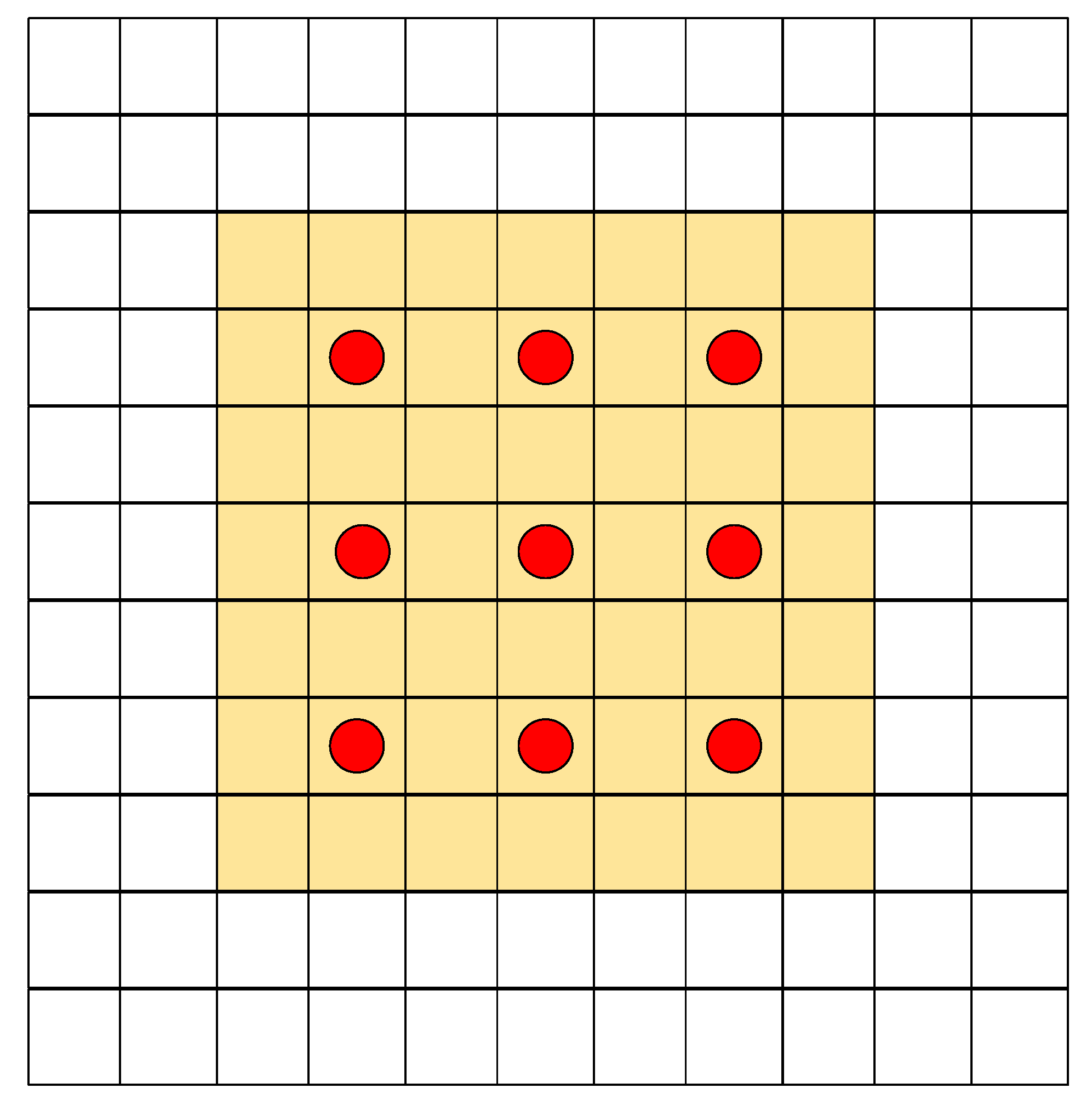
2.1.2. Dilated Convolution

Dilated convolution, also known as expanded convolution, is a convolution operation in CNN [36]. Dilated convolution introduces a controllable expansion parameter based on traditional convolution operations, allowing the network to have a larger receptive field and a wider perceptual range without increasing the number of parameters [36]. Figure 3 illustrates dilated convolution with a receptive field size of seven. By increasing the dilation rate parameter without altering the number of convolution kernels, dilated convolution exponentially expands the receptive field size, enabling each convolution layer’s output to incorporate a broader range of information.

The large expansion rate parameter enables the output of the top layer of the network to cover a larger range of inputs, effectively expanding the receptive field of the convolutional network. Expanding the receptive field can be achieved by increasing the size of the convolution kernel $k$ and the dilation rate parameter $d$. The receptive field size of the $n$-th layer is [36]:

$$r_n=r_{n-1}+d(k_n-1)\prod _{i=1}^{n-1}{s}_i$$

(2)

where $k_n$ is the n-th convolution kernel and ${\displaystyle \prod _{i=1}^{n-1}}{s}_i$ is the accumulated offset of each convolution kernel expanding outward.

When applying dilated convolution in TCN, the dilation rate parameter $d$ increases exponentially as the network depth deepens, ensuring the convolution kernel can hit each valid historical input. Meanwhile, dilated convolution enables deep networks to remember input information, which is very distant and effectively alleviates the training difficulties caused by the large computational complexity of causal convolution operations.

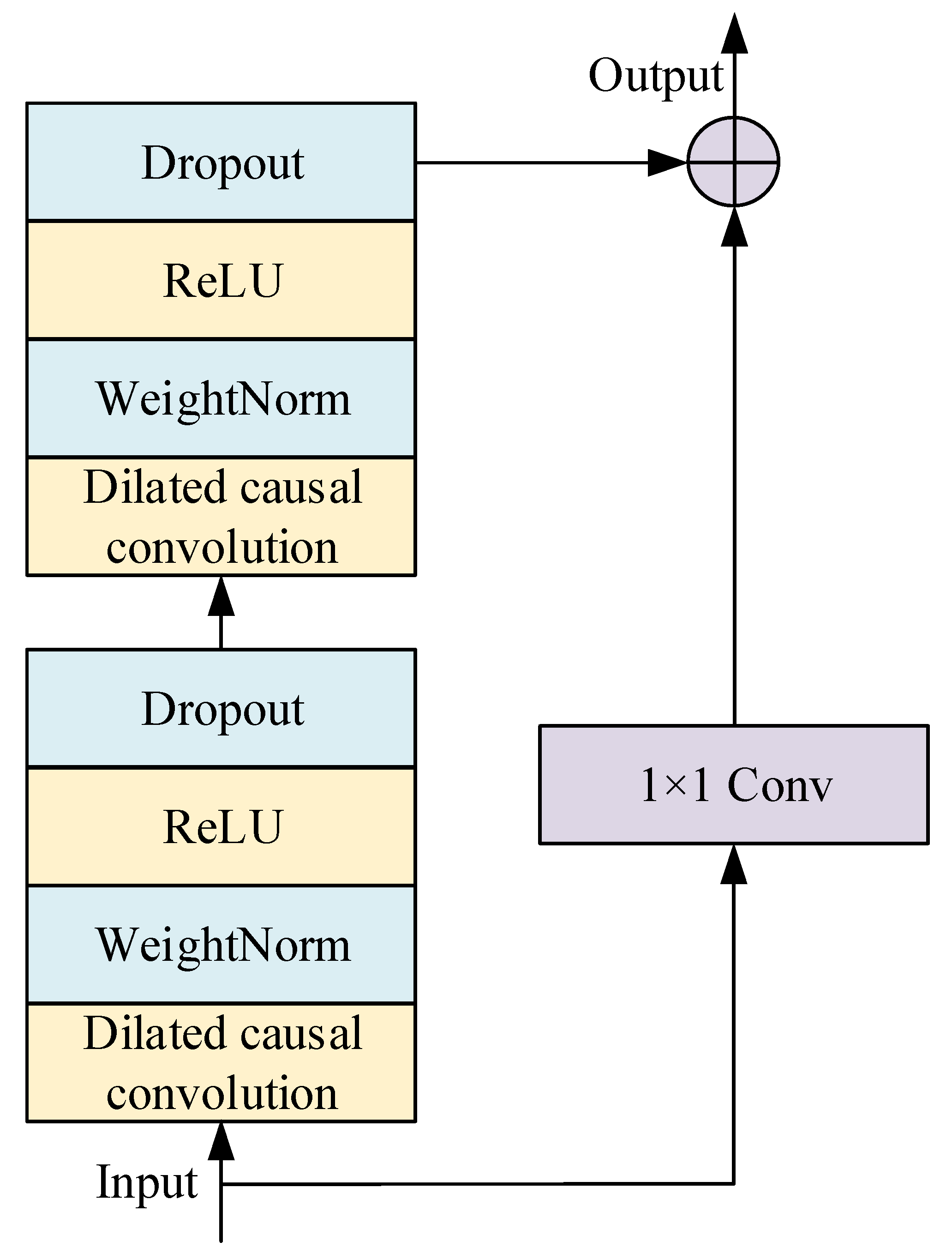
2.1.3. Residual Connection

Residual connection in TCN is a technique applied to enhance network performance. Residual connection adds the output of the convolutional layer to the initial input, enabling smoother information transmission and backpropagation, which helps to alleviate the problem of gradient vanishing and accelerate training convergence (Figure 4) [37]. Residual connection can improve the long-term dependency and representation ability of the model, enabling TCN to better process time series data.

The input–output relationship of the residual connection is [37]:

$$H(x)=F(x)+x$$

(3)

where $H(x)$ is the output of residual connection, $F(x)$ is the output of convolution, and $x$ is the input of residual connection.

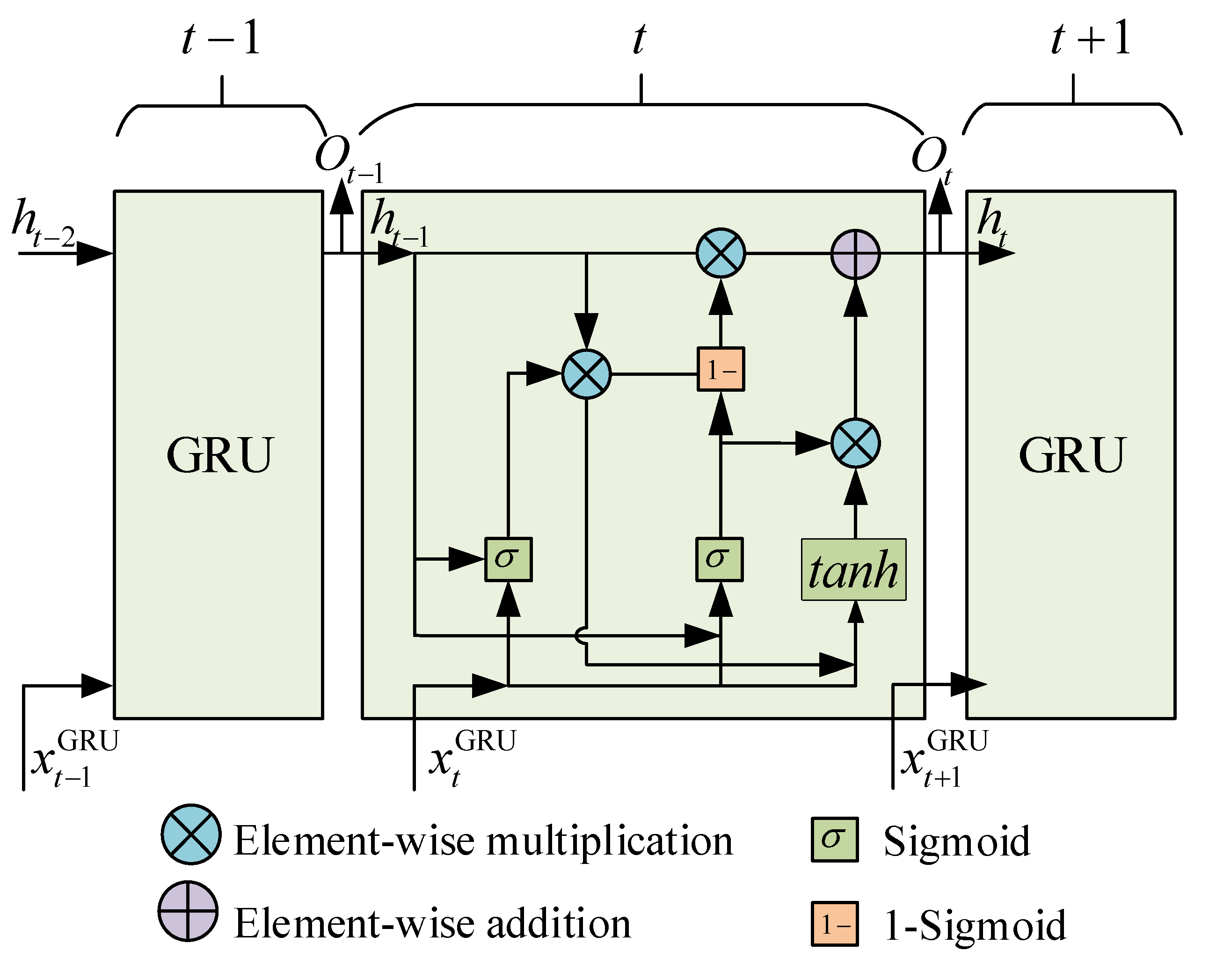
2.2. Gated Recurrent Unit

LSTM has improved RNN by altering the internal structure of neurons. The input data information is constrained by the cell state to save the valid data, pass valid data on, and eliminate the invalid and redundant information [38]. Since LSTM solves the gradient problem in RNN well and obtains great prediction results, LSTM has been popularized in various fields. However, the introduction of cell state increases the number of training parameters and the difficulty of training, reducing the speed of prediction [38]. To improve the computational speed of LSTM, it is necessary to simplify the internal components of recurrent structure as much as possible while ensuring computational efficiency. Therefore, some scholars have proposed GRU (Figure 5).

GRU can learn long-range temporal features by controlling update and reset gates for determining the degree of preservation and forgetting of neuronal information [39].

2.2.1. Update Gate and Reset Gate

The reset gate and update gate inputs of GRU are the current input and the previous hidden layer output, which are fully connected through sigmoid. Therefore, the output range of GRU is 0 to 1, and the outputs of the reset gate and update gate are [39]:

$$r_{\mathrm{t}}=\sigma (w_{\mathrm{rx}}{x}_{\mathrm{t}}+w_{\mathrm{rh}}{h}_{\mathrm{t}-1}+b_{\mathrm{r}})$$

(4)

$$z_{\mathrm{t}}=\sigma (w_{\mathrm{zx}}{x}_{\mathrm{t}}+w_{\mathrm{zh}}{h}_{\mathrm{t}-1}+b_z)$$

(5)

where $\sigma$ is the activation function of sigmoid; $h_{\mathrm{t}-1}$ is the output of the hidden layer from the previous time; $x_{\mathrm{t}}$ is the current time input; $w_{\mathrm{rx}}$ and $w_{\mathrm{rh}}$ are the weights of the reset gate input and hidden state, respectively; $w_{\mathrm{zx}}$ and $w_{\mathrm{zh}}$ are the weights of the update gate input and hidden state, respectively; $b_{\mathrm{r}}$ and $b_z$ are the biases of the reset gate and the update gate, respectively; $r_{\mathrm{t}}$ is the reset door; and $z_{\mathrm{t}}$ is the update gate.

2.2.2. Candidate Hidden State and Hidden State

The key difference between RNN and GRU lies in the fact that the latter incorporates gating mechanisms for its hidden states. GRU has specialized mechanisms to determine when the hidden state should be updated and reset. The hidden state in GRU carries the memory of network and the comprehensive understanding of sequential data and adjusts through update gates to fuse past information. The candidate hidden state is the previous value at the current time step, regulated by the reset gate and employed to capture crucial features of the current input. The candidate hidden state and hidden state of GRU are [39]:

$${\tilde{h}}_{\mathrm{t}}=Tanh(w_{\widetilde{\mathrm{hx}}}{x}_{\mathrm{t}}+w_{\widetilde{\mathrm{hh}}}(r_{\mathrm{t}}\odot h_{t.1})+b_{\tilde{\mathrm{h}}})$$

(6)

$$h_{\mathrm{t}}=(1-z_{\mathrm{t}})\odot h_{\mathrm{tl}}+z_{\mathrm{t}}\odot {\tilde{h}}_{\mathrm{t}}$$

(7)

where $w_{\widetilde{\mathrm{hx}}}$ and $w_{\widetilde{\mathrm{hh}}}$ are the weight matrices of candidate vectors for input and hidden layers, respectively; ${\tilde{h}}_{\mathrm{t}}$ is the output of candidate hidden states; $h_{\mathrm{t}}$ is the output of the hidden layer at the current time; and $\odot$ is the multiplication of the corresponding elements.

2.3. Attention Mechanism

The attention mechanism is a method inspired by human attention allocation, widely applied in deep learning models, particularly suitable for processing time series data [40]. The core concept of the attention mechanism is that the model can selectively focus on certain important parts when processing input data while ignoring relatively unrelated parts [40]. The attention mechanism enables the model to dynamically allocate attention based on different contexts, thereby improving model performance and accuracy. Introducing the attention mechanism into deep learning models can help reduce data redundancy and repetition. The attention mechanism calculates the attention weights of each part of the input data, allowing the model to more effectively focus on key information rather than uniformly processing all inputs.

This study adopted a GRU-based attention model, where the GRU was applied to extract global features from temporal data and the attention mechanism was applied to calculate the correlation between each input and output and generate attention weights based on the correlation. Then, we multiplied the attention weights by the output of the GRU to obtain the GRU output value after incorporating the attention mechanism (Figure 6).

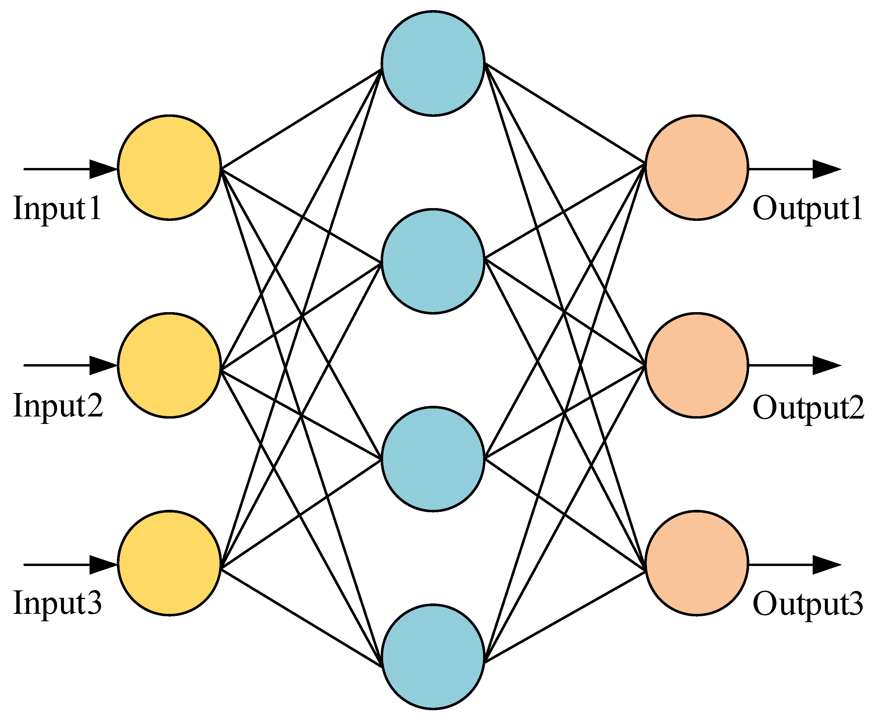
2.4. Multilayer Perceptron

Multilayer perceptron (MLP) is a feedforward neural network with an input layer, one or more hidden layers, and an output layer. Each neuron computes a weighted sum of its inputs and applies a nonlinear activation function. During training, weights are adjusted through backpropagation to minimize the error between predicted and actual outputs, allowing the MLP to learn complex patterns in the data (Figure 7). The reason why MLP is called “multilayer” is because MLP contains multiple hidden layers, allowing the model to learn more complex features and representations [41].

2.5. TCN-GRU-Attention-MLP

This study proposed a hybrid model based on TCN, GRU, attention mechanism, and MLP for predicting long-term GHI. TGAM mainly includes the following three parts: data processing, model training, and testing (Figure 8). Firstly, the data processing section applied a Spearman correlation coefficient analysis to screen solar radiation and related features, obtaining features with a high correlation to solar radiation. Then, the data were divided into training, validation, and testing sets. The processed training set was input into the model training section of the parallel GRU and TCN, where the output of the GRU needed to pass through an attention layer to highlight important features. The MLP fit the outputs of the GRU and TCN to obtain the final prediction result and obtained the optimal model through the validation set. The last part was the testing section. The test set was input into TGAM with the best parameters, and then the performance of the model was validated through three evaluation metrics: mean absolute error (MAE), mean absolute percentage error (MAPE), and root mean square error (RMSE).

3. Case Analysis

Current GHI correlation datasets are mostly sampled at a resolution of 15 min or 1 h for short-term data. However, if we want to predict the GHI for the preliminary siting of PV power plants, the short sampling frequency of the data is difficult to fulfill. Therefore, in this study, data in minutes and hours were integrated into data in days by integrating and processing the data, thus fitting the need for long-term data for PV plant siting. This study utilized a time series dataset collected from multiple solar irradiance measurement points, including locations in the United States, Mexico, Karachi, Lahore, Islamabad, Peshawar, İzmir, and Almería. The sampling resolution was 1 h for the United States and Mexico and 15 min for Karachi, Lahore, Islamabad, Peshawar, İzmir, and Almería. Since solar radiation was only present during the daytime, this study considered data from 8 a.m. to 5 p.m. each day. Due to the low sampling resolution of the collected data, the study processed the data to achieve a daily sampling resolution. For the hourly data, the study summed the values to obtain daily data; for the 15 min resolution data, it first computed the sum and then averaged it to obtain hourly data, which were subsequently summed to produce daily data. And then, we predicted the future GHI for the next 7 days based on the past 15 days of data. The time series dataset included features such as longitude and latitude, altitude, wind speed, humidity, global horizontal irradiance (GHI), direct normal irradiance (DNI), and diffuse horizontal irradiance (DHI). The allocation ratios for the training set, validation set, and test set in this study were 70%, 10%, and 20%.

3.1. Evaluation Metric

This study applied three different evaluation metrics, MAE, MAPE, and RMSE, which measured the difference between predicted and true values to quantify the performance of model predictions [42]:

$$E_{\mathrm{RMSE}}=\sqrt{{\displaystyle \frac{1}{N}}\sum _{i=1}^N{(y_i^{\ast }-y_i)}^2}$$

(8)

$$E_{\mathrm{MAE}}={\displaystyle \frac{1}{N}}\sum _{i=1}^N|y_i^{\ast }-y_i|$$

(9)

$$E_{\mathrm{MAPE}}={\displaystyle \frac{100\%}{N}}\sum _{i=1}^N\left|{\displaystyle \frac{y_i^{\ast }-y_i}{y_i}}\right|$$

(10)

where $N$ is the number of samples; $y_i^{\ast }$ is the $i$-th predicted value; and $y_i$ is the $i$-th true value.

3.2. Parameter Setting

This study applied optuna from the Python library to search for the optimal parameters [43]. The main role of optuna is to automate hyperparameter optimization and thus improve the performance of the model. A parameter search range was set for the number of training epochs, learning rate, and all optimizable parameters in TGAM for the model. The best parameters were then found through optimization measures such as Bayesian optimization by optuna. Optuna avoided the tedious process of manually tuning the hyperparameters and significantly saving time and computational resources. The optimal model was applied to predict GHI. The optimal model parameters are shown in

Table 1. Optimal model parameters.

Algorithm	Parameter	Value
TCN	Channel	[80,128,176]
	Kernel size	3
	Dropout	0.4
	Dilation size	2
GRU	Hidden units	32
	Hidden layers	5
MLP	Hidden units	[128,160]
	Hidden layers	2

; epoch was 200, learning rate was 0.001, optimizer was Adam, and batch size was 160.

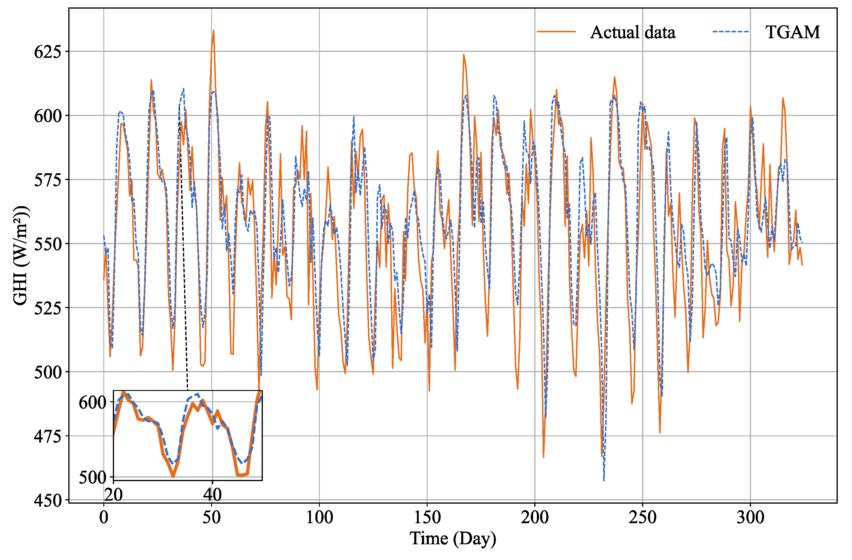
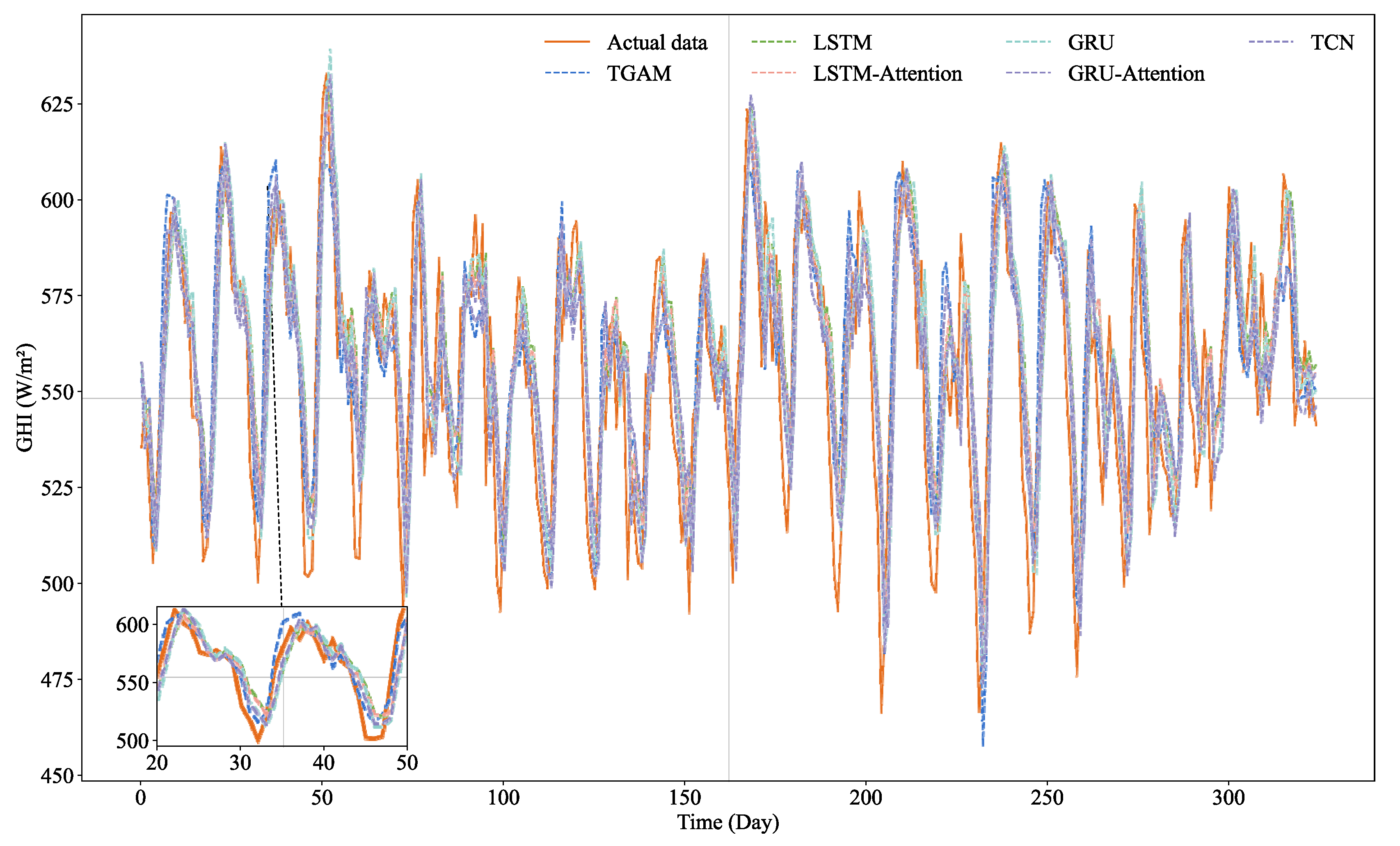
3.3. Result Analysis

This study validated the model using a validation set and obtained the optimal parameters. The test set was fed into the optimal model to predict GHI. The comparison curve between the predicted results of the TGAM model and the real data is shown in Figure 9. The predicted results of the TGAM model, which were roughly consistent with the trend of real data, effectively predicted the trend of GHI changes.

To verify the superiority of the proposed TGAM in the GHI prediction, this study compared TGAM with LSTM, LSTM-Attention, GRU, GRU-Attention, and TCN. The data of the above comparison algorithms were preprocessed applying max–min normalization, and the optimal parameters were obtained by applying the open-source machine learning library optuna.

Although the predicted values of LSTM, LSTM-Attention, GRU, GRU-Attention, and TCN closely matched the real values, the proposed TGAM demonstrated a superior performance, exhibiting predictions that were even more closely aligned with the real values (Figure 10).

Figure 11 and

Table 2. The evaluation indicators between the TGAM and comparison algorithms.

Algorithm	MAE	MAPE	RMSE
LSTM	18.8	0.034	23.07
LSTM-Attention	17.53	0.032	21.77
GRU	18.61	0.033	22.53
GRU-Attention	16.92	0.03	20.84
TCN	16.66	0.03	20.75
TGAM	12.6	0.02	15.7

show the evaluation metrics (MAE, MAPE, and RMSE) and improvement percentages of the proposed TGAM and compared algorithms. Columns represent the evaluation metrics of the algorithm; the line represents the percentage improvement achieved by the proposed TGAM compared to the comparison algorithm. The proposed TGAM had the smallest MAE, MAPE, and RMSE. Compared with the comparison algorithm, the proposed TGAM was 24.4% smaller than the second smallest TCN in MAE, 33% smaller than the largest LSTM in MAE, 33.33% smaller than the second smallest TCN and GRU-Attention in MAPE, 41.2% smaller than the largest LSTM in MAPE, 24.3% smaller than the second smallest TCN in RMSE, and 32% smaller than the largest LSTM in RMSE.

Both LSTM and GRU had improved performance when combined with Attention. LSTM-Attention had improved MAE, MAPE, and RMSE by 7%, 6%, and 7%, respectively, compared to LSTM. Compared to GRU, GRU-Attention had improved MAE, MAPE, and RMSE by 9%, 9%, and 8%, respectively.

4. Discussions

Considering actual photovoltaic power stations are distributed solar sites, the features applied in this study are challenging to obtain simultaneously. This study analyzed the impact of different input feature deletions on the predictive performance of the proposed TGAM model (Figure 12). DHI represented the missing input variable DHI, and the remaining five variables on the horizontal axis were applied as model inputs. Similar to DHI, Longitude, Latitude, Altitude, DNI, GHI, Humidity, Temperature, and Windspeed represented the missing variables as Longitude, Latitude, Altitude, GHI, Humidity, Temperature, and Windspeed, respectively. All means applied the six variables mentioned above as inputs to the model.

When the input variable lacked GHI, the TGAM model performed the worst in all three evaluation metrics: MAE, MAPE, and RMSE. Therefore, GHI was the variable with the greatest impact on performance among all variables. When all of the aforementioned six variables were applied as model inputs, the predictive performance reached optimal levels. The absence of any variable resulted in a decrease in the performance of the three evaluation indicators of the model, which indicated that the relevant features in the data contributed to improving the accuracy of the model prediction.

5. Conclusions

This study proposes a hybrid model based on TCN, GRU, attention mechanism, and MLP for predicting long-term GHI, providing guidance for the selection of photovoltaic power plant locations. TCN and GRU Attention form a parallel network to predict the input data and then send the prediction results together into MLP to obtain the final prediction result. According to the three evaluation indicators, MAE, MAPE, and RMSE, the proposed model achieved better results compared to the comparative algorithms. The main conclusions of this study are as follows:

(1)

The proposed TGAM model integrates TCN and GRU, combining the characteristics of CNN and RNN. TCN extracts deep features of solar radiation, while GRU captures long-term dependencies of solar radiation time series. Two different types of algorithms complement each other to improve the overall prediction accuracy of the model.

(2)

The combination of GRU and attention mechanism enables the model to dynamically adjust attention levels based on different parts of the input sequence, improving model performance.

(3)

Compared to simply adding up the prediction results of TCN and GRU, this study utilizes MLP to adaptively adjust the weight coefficients of TCN and GRU, thereby avoiding the inclusion of algorithms with poor performance and improving the overall model prediction accuracy.

(4)

In addition to considering the relevant characteristics, which affect solar radiation, this study considers the Map distribution features, i.e., latitude, longitude, and altitude, providing a reference basis for the selection of photovoltaic power stations.

References

1. Feng, T.; Li, R.; Zhang, H. Induction mechanism and optimization of tradable green certificates and carbon emission trading acting on electricity market in China. Resour. Conserv. Recycl. 2021, 169, 105487. [Google Scholar] [CrossRef]
2. National Energy Administration Releases 2022 National Electric Power Industry Statistical Data. Available online: http://www.nea.gov.cn/2023-01/18/c_1310691509.htm (accessed on 30 June 2023).
3. Liu, B.; Huo, X. Prediction of Photovoltaic power generation and analyzing of carbon emission reduction capacity in China. Renew. Energy 2024, 222, 119967. [Google Scholar] [CrossRef]
4. Lai, C.S.; Zhong, C.; Pan, K. A deep learning based hybrid method for hourly solar radiation forecasting. Expert Syst. Appl. 2021, 177, 114941. [Google Scholar] [CrossRef]
5. Jiang, Y.; Long, H.; Zhang, Z. Day-ahead prediction of bihourly solar radiance with a Markov switch approach. IEEE Trans. Sustain. Energy 2017, 8, 1536–1547. [Google Scholar] [CrossRef]
6. Sansa, I.; Boussaada, Z.; Bellaaj, N.M. Solar radiation prediction using a novel hybrid model of ARMA and NARX. Energies 2021, 14, 6920. [Google Scholar] [CrossRef]
7. García-Cuesta, E.; Aler, R.; Pózo-Vázquez, D. A combination of supervised dimensionality reduction and learning methods to forecast solar radiation. Appl. Intell. 2023, 53, 13053–13066. [Google Scholar] [CrossRef]
8. Narvaez, G.; Giraldo, L.F.; Bressan, M. Machine learning for site-adaptation and solar radiation forecasting. Renew. Energy 2021, 167, 333–342. [Google Scholar] [CrossRef]
9. Gaviria, J.F.; Narváez, G.; Guillen, C.; Giraldo, L.F.; Bressan, M. Machine learning in photovoltaic systems: A review. Renew. Energy 2022, 196, 298–318. [Google Scholar] [CrossRef]
10. Alrashidi, M.; Alrashidi, M.; Rahman, S. Global solar radiation prediction: Application of novel hybrid data-driven model. Appl. Soft Comput. 2021, 112, 107768. [Google Scholar] [CrossRef]
11. Villegas-Mier, C.G.; Rodriguez-Resendiz, J.; Álvarez-Alvarado, J.M. Optimized random forest for solar radiation prediction using sunshine hours. Micromachines 2022, 13, 1406. [Google Scholar] [CrossRef]
12. Goliatt, L.; Yaseen, Z.M. Development of a hybrid computational intelligent model for daily global solar radiation prediction. Expert Syst. Appl. 2023, 212, 118295. [Google Scholar] [CrossRef]
13. Chaibi, M.; Benghoulam, E.M.; Tarik, L.; Berrada, M.; Hmaidi, A.E. An interpretable machine learning model for daily global solar radiation prediction. Energies 2021, 14, 7367. [Google Scholar] [CrossRef]
14. Zhou, Y.; Liu, Y.; Wang, D.; Liu, X.; Wang, Y. A review on global solar radiation prediction with machine learning models in a comprehensive perspective. Energy Convers. Manag. 2021, 235, 113960. [Google Scholar] [CrossRef]
15. Irshad, K.; Islam, N.; Gari, A.A.; Algarni, S.; Algahtani, T.; Imteyaz, B. Arithmetic optimization with hybrid deep learning algorithm based solar radiation prediction model. Sustain. Energy Technol. Assess. 2023, 57, 103165. [Google Scholar] [CrossRef]
16. Ehteram, M.; Shabanian, H. Unveiling the SALSTM-M5T model and its python implementation for precise solar radiation prediction. Energy Rep. 2023, 10, 3402–3417. [Google Scholar] [CrossRef]
17. Vural, N.M.; Ilhan, F.; Yilmaz, S.F.; Ergüt, S.; Kozat, S.S. Achieving online regression performance of LSTMs with simple RNNs. IEEE Trans. Neural Netw. Learn. Syst. 2021, 33, 7632–7643. [Google Scholar] [CrossRef]
18. Zhaowei, Q.; Haitao, L.; Zhihui, L.; Tao, Z. Short-term traffic flow forecasting method with MB-LSTM hybrid network. IEEE Trans. Intell. Transp. Syst. 2020, 23, 225–235. [Google Scholar] [CrossRef]
19. Zarzycki, K.; Ławryńczuk, M. Advanced predictive control for GRU and LSTM networks. Inf. Sci. 2022, 616, 229–254. [Google Scholar] [CrossRef]
20. Imani, M. Electrical load-temperature CNN for residential load forecasting. Energy 2021, 227, 120480. [Google Scholar] [CrossRef]
21. Wang, Z.; Peng, X.; Cao, S.; Zhou, H.; Fan, S.; Li, K.; Huang, W. NOx emission prediction using a lightweight convolutional neural network for cleaner production in a down-fired boiler. J. Clean. Prod. 2023, 389, 136060. [Google Scholar] [CrossRef]
22. Ghimire, S.; Deo, R.C.; Casillas-Pérez, D.; Salcedo-Sanz, S.; Sharma, E.; Ali, M. Deep learning CNN-LSTM-MLP hybrid fusion model for feature optimizations and daily solar radiation prediction. Measurement 2022, 202, 111759. [Google Scholar] [CrossRef]
23. Ghimire, S.; Bhandari, B.; Casillas-Perez, D.; Deo, R.C.; Salcedo-Sanz, S. Hybrid deep CNN-SVR algorithm for solar radiation prediction problems in Queensland, Australia. Eng. Appl. Artif. Intell. 2022, 112, 104860. [Google Scholar] [CrossRef]
24. Yang, W.; Xia, K.; Fan, S. Oil logging reservoir recognition based on TCN and SA-BiLSTM deep learning method. Eng. Appl. Artif. Intell. 2023, 121, 105950. [Google Scholar] [CrossRef]
25. Zhang, C.; Li, J.; Huang, X.; Zhang, J.; Huang, H. Forecasting stock volatility and value-at-risk based on temporal convolutional networks. Expert Syst. Appl. 2022, 207, 117951. [Google Scholar] [CrossRef]
26. Ni, S.; Jia, P.; Xu, Y.; Zeng, L.; Li, X.; Xu, M. Prediction of CO concentration in different conditions based on Gaussian-TCN. Sens. Actuators B Chem. 2023, 376, 133010. [Google Scholar] [CrossRef]
27. Tian, C.; Niu, T.; Wei, W. Developing a wind power forecasting system based on deep learning with attention mechanism. Energy 2022, 257, 124750. [Google Scholar] [CrossRef]
28. Gao, Y.; Miyata, S.; Akashi, Y. Interpretable deep learning models for hourly solar radiation prediction based on graph neural network and attention. Appl. Energy 2022, 321, 119288. [Google Scholar] [CrossRef]
29. Kong, X.; Du, X.; Xue, G.; Xu, Z. Multi-step short-term solar radiation prediction based on empirical mode decomposition and gated recurrent unit optimized via an attention mechanism. Energy 2023, 282, 128825. [Google Scholar] [CrossRef]
30. Rajasundrapandiyanleebanon, T.; Kumaresan, K.; Murugan, S.; Subathra, M.S.P.; Sivakumar, M. Solar energy forecasting using machine learning and deep learning techniques. Arch. Comput. Methods Eng. 2023, 30, 3059–3079. [Google Scholar] [CrossRef]
31. Lee, J.A.; Dettling, S.M.; Pearson, J.; Brummet, T.; Larson, D.P. NYSolarCast: A solar power forecasting system for New York State. Sol. Energy 2024, 272, 112462. [Google Scholar] [CrossRef]
32. Deveci, M.; Pamucar, D.; Oguz, E. Floating photovoltaic site selection using fuzzy rough numbers based LAAW and RAFSI model. Appl. Energy 2022, 324, 119597. [Google Scholar] [CrossRef]
33. Elmousaid, R.; Drioui, N.; Elgouri, R.; Agueny, H.; Adnani, Y. Ultra-short-term global horizontal irradiance forecasting based on a novel and hybrid GRU-TCN model. Results Eng. 2024, 23, 102817. [Google Scholar] [CrossRef]
34. Yin, L.; Zhou, H. Modal decomposition integrated model for ultra-supercritical coal-fired power plant reheater tube temperature multi-step prediction. Energy 2024, 292, 130521. [Google Scholar] [CrossRef]
35. Yin, L.; Xie, J. Multi-feature-scale fusion temporal convolution networks for metal temperature forecasting of ultra-supercritical coal-fired power plant reheater tubes. Energy 2022, 238, 121657. [Google Scholar] [CrossRef]
36. Hao, J.; Liu, F.; Zhang, W. Multi-scale RWKV with 2-dimensional temporal convolutional network for short-term photovoltaic power forecasting. Energy 2024, 309, 133068. [Google Scholar] [CrossRef]
37. Li, Y.; Song, L.; Zhang, S.; Kraus, L.; Adcox, T.; Willardson, R.; Komandur, A.; Komandur, A.; Lu, N. A TCN-based hybrid forecasting framework for hours-ahead utility-scale PV forecasting. IEEE Trans. Smart Grid 2023, 14, 4073–4085. [Google Scholar] [CrossRef]
38. Li, Q.; Guan, X.; Liu, J. A CNN-LSTM framework for flight delay prediction. Expert Syst. Appl. 2023, 227, 120287. [Google Scholar] [CrossRef]
39. Gupta, U.; Bhattacharjee, V.; Bishnu, P.S. StockNet—GRU based stock index prediction. Expert Syst. Appl. 2022, 207, 117986. [Google Scholar] [CrossRef]
40. Xu, Y.; Zheng, S.; Zhu, Q.; Wong, K.C.; Wang, X.; Lin, Q. A complementary fused method using GRU and XGBoost models for long-term solar energy hourly forecasting. Expert Syst. Appl. 2024, 254, 124286. [Google Scholar] [CrossRef]
41. Mobarakeh, J.M.; Sayyaadi, H. A novel methodology based on artificial intelligence to achieve the formost Buildings’ heating system. Energy Convers. Manag. 2023, 286, 116958. [Google Scholar] [CrossRef]
42. Yin, L.; Wei, X. Integrated adversarial long short-term memory deep networks for reheater tube temperature forecasting of ultra-supercritical turbo-generators. Appl. Soft Comput. 2023, 142, 110347. [Google Scholar] [CrossRef]
43. Akiba, T.; Sano, S.; Yanase, T.; Ohta, T.; Koyama, M. Optuna: A next-generation hyperparameter optimization framework. In Proceedings of the 25th ACM SIGKDD International Conference on Knowledge Discovery & Data Mining, Anchorage, AK, USA, 4–8 August 2019; pp. 2623–2631. [Google Scholar]
Figure 1. The framework diagram of TCN.
Energies 17 05767 g001
Figure 2. The framework diagram of causal convolution.
Energies 17 05767 g002
Figure 3. The framework diagram of dilated convolution.
Energies 17 05767 g003
Figure 4. The framework diagram of residual connection.
Energies 17 05767 g004
Figure 5. The framework diagram of GRU.
Energies 17 05767 g005
Figure 6. The framework diagram of attention mechanism.
Energies 17 05767 g006
Figure 7. The framework diagram of MLP.
Energies 17 05767 g007
Figure 8. The framework diagram of TGAM.
Energies 17 05767 g008
Figure 9. The prediction fitting plot of TGAM.
Energies 17 05767 g009
Figure 10. The prediction fitting plot of TGAM and comparison algorithms.
Energies 17 05767 g010
Figure 11. The evaluation indicators and improvement percentages of TGAM and comparison algorithms: (a) MAE; (b) MAPE; (c) RMSE.
Energies 17 05767 g011
Figure 12. The impact of missing variables on model prediction: (a) MAE; (b) MAPE; (c) RMSE.
Energies 17 05767 g012