1. Introduction
To substantially reduce CO
2 emissions, energy production from renewable energy sources (RESs) needs to be dramatically increased [
1,
2]. A large share of renewable energy production is expected from wind and photovoltaics (PV), e.g., [
3,
4], with PV investment already surpassing all other power generation technologies (including fossil) combined [
5].
In addition to RESs, hydrogen usage plays a crucial role in achieving CO
2 emission targets, e.g., [
6,
7]. Hydrogen can be produced through electrolysis using RESs, e.g., [
8,
9]. Numerous studies discuss the emergence of a hydrogen market, leading to local production within Europe and imports from other regions, e.g., [
10,
11]. Transporting hydrogen to Europe can be done via pipelines or ships. For shorter distances, pipeline transport is more cost-effective due to the absence of conversion costs, e.g., [
12,
13]. While hydrogen production per installed PV and wind capacity may be higher outside Europe, economic assessments must consider factors such as the weighted average cost of capital (WACC) in specific countries [
14,
15], as well as transport and conversion costs until delivery in Europe, e.g., [
16,
17,
18]. Geopolitical considerations and energy security also influence the choice between locally produced and imported hydrogen, e.g., [
19,
20]. Additionally, addressing hydrogen losses during long-distance transportation and conversion projects is important, along with determining their potential impact on global warming, e.g., [
21,
22,
23].
Greenhouse gas emissions need to be considered for the production of hydrogen. The lowest greenhouse gas emissions occur when RESs are used for hydrogen generation [
8]. To generate hydrogen, researchers have analyzed the interactions of wind, PV, and electrolyzers in various contexts. Al-Ghussain et al. [
24] studied these interactions in Jordan, while Di Lorenzo et al. [
25] focused on Saudi Arabia. Yates et al. [
26] introduced uncertainty into their analysis of PV and electrolysis. Additionally, Povacz and Bhandari [
27] examined an off-grid PV–wind–electrolysis system in Austria, and Radner et al. [
28] investigated grid-supporting electrolysis.
In addition to its applications in various industrial processes such as steel production, fertilizer manufacturing, and cement industry, e.g., [
29], hydrogen also plays a crucial role in seasonal energy storage, e.g., [
30,
31]. The reason is that increasing the contribution of fluctuating RESs such as wind and PV to the total energy production leads to challenges in the distribution and oversupply of energy. Short and seasonal energy storage as well as grid stabilization need to be considered, e.g., [
32,
33]. For short-term electricity storage, several options are available, e.g., [
34]. These solutions include various technologies such as thermal, mechanical, chemical, electrochemical, and hybrid systems, e.g., [
35,
36,
37,
38]. However, long-term (seasonal) electricity storage requires the conversion of electricity to hydrogen and underground storage, e.g., [
39,
40]. When used for seasonal energy storage, hydrogen is injected during periods of excess electricity availability and produced during times of high hydrogen and electricity demand, e.g., [
41,
42]. In underground hydrogen storage (UHS), several processes need to be considered, such as hydrogen–rock interactions, microbial growth within reservoirs, and geomechanical effects, e.g., [
43,
44,
45]. Particularly important is the mixing of hydrogen with hydrocarbon gases present in depleted gas reservoirs or reservoirs used for underground (hydrocarbon) gas storage [
46,
47,
48]. The mixing of hydrogen with hydrocarbon gases—or other gases used as cushion gas, e.g., [
49,
50]—will lead to the production of gas mixtures that need to be separated to achieve the required hydrogen purity, resulting in substantial costs, e.g., [
51,
52].
Here, we are showing the impact of electricity costs—constant and including price curves—and the effect of various wind-to-PV ratios on electrolyzer sizing for underground hydrogen storage (UHS) operations. Furthermore, we are covering the levelized costs of UHS.
The paper is organized as follows. First, we describe the methodology; then, we discuss the simulation model followed by the simulation results. Afterwards, economics are covered for fixed electricity prices and fluctuating electricity prices.
2. Methodology
Three different components are crucial for the overall system of sustainable energy generation and seasonal energy storage: (1) renewable energy generation, (2) electrolysis, and (3) underground hydrogen storage (UHS). The three topics and their associated levelized costs are introduced separately.
Figure 1 shows the setup of energy generation and conversion into hydrogen used here.
For renewable energy generation, variations of the installed capacity of PV versus wind energy were introduced. Hydrogen is generated throughout the entire year and during six months, particularly during summer, the hydrogen is injected into a subsurface reservoir. For the case study in Austria shown here, the hydrogen is pressurized to 60 bar(g) for export into a pipeline. The produced hydrogen from the subsurface reservoir is treated to meet pipeline specifications.
In the following sections, first, the overall setup is described, then, renewable energy generation is covered, followed by hydrogen generation, UHS, and economic evaluation.
2.1. Renewable Energy Generation
We have chosen an area in Eastern Austria to simulate electricity generation using wind and PV. The reference weather data location was Fischamend in Austria (coordinates: 48.100278, 16.637361). For wind energy, the INCA hourly data (INCA Stundendaten) provided by GeoSphere Austria (
https://data.hub.geosphere.at/dataset/inca-v1-1h-1km, accessed on 20 July 2024) were used. For solar radiation, the Photovoltaic Geographical Information System (PV-GIS) with PVGIS-SARAH2 as a database was used (
https://re.jrc.ec.europa.eu/pvg_tools/en/, accessed on 15 June 2024). As time period, 1 January 2019–31 December 2019 (hourly steps) was applied.
Renewable energy generation by PV is covered in the next section, followed by the setup for wind energy.
2.1.1. Photovoltaic
Installation of agri-photovoltaic (agri-PV) was assumed for the project as agri-PV and allows to produce electricity while continuing agricultural activities, with adaptions due to partial shading [
53]. Here, we used a mixture of bifacial vertical and horizontal panels. In total, three modules were included in the simulation: (1) inclined (20°) modules facing south, (2) vertical modules facing east, and (3) vertical modules facing west. The bifacial module was defined to be the sum of the vertical east- and west-facing modules. For solar energy generation, a mix of 50% south-facing and 50% bifacial modules were assumed. Applying the mix and configuration, the resulting energy production was calculated. The reason for introducing a mixture of agrivoltaics and horizontal panels is that instead of a single peak of PV energy generation for panels facing south, a smoothed curve with lower maximum energy generation but more constant energy production extending further into the morning and afternoon can be achieved.
Figure 2 shows the energy production for a sunny winter day. An approach similar to that of Reker et al. [
54] was introduced. The blue line shows the energy generation for panels facing south resulting in a higher peak energy production than bifacial panels in the east-west direction (orange curves). The green curve shows the power output for the combined installation. Furthermore, social acceptance for solar power generation is increased if agrivoltaics is used, as conflicts of land use for PV and agriculture are reduced [
55]. The energy production for the vertical panels was 400–500 kWp/ha, whereas, for horizontally inclined panels, it was 1750 kWp/ha.
2.1.2. Wind Energy
The wind velocity in the weather data was given for 10 m above ground level. The wind velocity at the rotor hub at a height of 120 m was calculated according to the Hellman exponential law [
56]:
h—Height (m)
vh—Wind speed (m/s) at height h
v10—Wind speed (m/s) at height 10 m
The exponent of 0.16 was chosen according to Kleemann et al. [
57] for open terrain with few obstacles. The power generation was simulated based on a power curve for the wind turbines [
58], with corresponding cut-in and cut-out wind velocities. For further details, refer to
Section 2.4 and
Appendix A.
2.2. Hydrogen Generation
To generate hydrogen, installation of a current industry standard proton-exchange membrane (PEM) electrolyzer was assumed. The PEM’s size and power were estimated through simulations of a generalized PEM model (see
Section 2.4) based on a targeted annual hydrogen output of approximately 20,000 t. Assuming an initial system efficiency of 53.3 kWh/kg of hydrogen produced led to a PEM size and power rating of 265 MW. The electrolyzer size was used in the model throughout the investigations herein; however, the system efficiency considered for the economic calculations was set to 54.15 kWh/kg to represent a more realistic average value.
The PEM electrolyzer system was assumed to be made up of individual package units with a power rating of 10 to 15 MW each, but in the simulation model, only the maximum power consumption of 265 MW needed to be considered. Since, in a realistic system, every electrolyzer unit has a certain turn-down ratio, limiting operation to a minimum required power input, the PEM for the simulation model was specified to require at least 300 kW of power input to produce hydrogen. The pressure of the product gas was specified to be constant and at 30 bar(g). After the electrolyzer, the produced hydrogen was modelled to be prepared and compressed either for underground storage or for supply to a hydrogen pipeline at 60 bar(g).
2.3. Underground Hydrogen Storage
The hydrogen requires conditioning after being stored underground due to mixture with remaining gases in the reservoir. To separate the produced gases, the following key components are introduced: pressure swing adsorption (PSA), silica gel dryer, and membrane. The PSA is used to produce the hydrogen stream with high purity. The tail gas is further processed. The silica gel dryer is used to dry the gas mixture to avoid condensation on the membrane, which would significantly impact its performance negatively. The water from the regeneration of the dryer is fed into the PSA. Water is condensed from the gas phases in compressors and removed from the system.
Compressors were simulated to assess power and cooling demand, with a maximum pressure ratio per stage of 3.
Figure 3 provides an overview of the process and indicates where compressors are required. Compressors are required to achieve desired pressure levels for conditioning and meet feed-in requirements for the grids.
The membrane is used to achieve a maximum hydrogen content (max. 2 vol%) resulting in gas mixtures that can be fed into a natural gas pipeline. Hydrogen permeates through the membrane, leading to an enrichment of methane in the retentate. The methane-rich retentate stream (high pressure) is fed to the natural gas grid. The hydrogen-rich permeate stream (low pressure) is compressed and recycled back to the PSA (refer to
Figure 3 for a process overview).
2.4. Simulation Model
To simulate hydrogen production under various conditions and system configurations, dynamic process simulation was used [
59].
Figure 4 shows the flowsheet including the various components of the simulation model applied for sustainable energy and hydrogen generation including grid return of excess electricity and water supply for electrolysis. Technical details of the considered agri-PV, wind, and electrolysis components are described in
Section 2.1 and
Section 2.2.
For the PV configuration of the solar farm, a 50:50 mix of panels was assumed: 50% of the panels were bifacial facing east and west, and 50% of the panels were inclined by 20% to the south. As described in
Section 2.1.1, this configuration was chosen due to its flattened electricity-production curve, resulting from the shift of peak power generation from noon to late forenoon and early afternoon by implementation of the vertical bifacial panels. The panel efficiency was assumed to be 21.2% and the temperature coefficient to be −0.47%/°C. Furthermore, only electrical losses (wiring, connections, etc.) and no degradation or environmental effects were considered for the solar farm. The efficiency of the inverter after the solar farm was calculated dynamically based on the load. More details about the photovoltaic model are given in
Appendix A.
The wind park model was assumed to be made up of individual 5 MW turbines with a blade length of 64 m each, a rated velocity of 14 m/s, a cut-in velocity of 2 m/s, and a cut-out velocity of 27 m/s.
Both power output lines from the renewable energy sources were first transformed to 20 kV. At this point, the model was set up to route excess electricity to the communal grid (grid return) when the electrolyzer (EY) is either operated at full capacity (265 MW), or the minimum required power input to the EY is not reached (300 kW). After the optional grid return, another transformation step, up to 33 kV, and a rectifier were implemented before the electrolyzer. The rectifier was set to operate at a constant efficiency of 99%, while the efficiency of the transformers was calculated dynamically based on their current load state. Lastly, 1% electrical transmission losses were assumed between the main components of the simulation model (PV, Wind, EY, and the power electronics).
2.5. UHS Model
The modelled process for UHS is shown in
Figure 3. The gas from the subsurface storage primarily consists of hydrogen, with small amounts of impurities (mainly CH
4). At the beginning of a dispensing period, the gas in the reservoir is at pressures larger than 60 bar(g) and can be extracted and conditioned without the use of additional compressors prior to the gas conditioning line. Over the annual production time, the pressure in the reservoir decreases. When the pressure drops below the operating threshold, re-pressurization with the compressors is necessary to achieve target pressure for gas conditioning. The purity of the hydrogen decreases also over time each period.
At the commencement of the production period, the impurity content is low, resulting in a tail gas with a high hydrogen content. To increase the hydrogen yield and increase the methane content in the tail gas, the tail gas stream is recycled after the PSA, to a certain extent. At the beginning of each period, the tail gas is recycled until the maximum impurity content and/or maximum volume flow into the PSA is reached. While all gas is recycled, the membrane is not used, i.e., the runtime of the PSA and subsequent process steps are not the same. Subsequently, the recycling stream is reduced to avoid exceeding the input parameters, especially the impurity content, of the PSA, leading to increasing volume flows to the dryer and membrane.
3. Simulation Results
In this section, first, the simulation results of energy generation using PV and wind energy and conversion into hydrogen for various installed capacities of the wind, PV, and electrolyzer are given. Then, we cover the simulation results for UHS.
3.1. Simulation of Sustainable Energy and Hydrogen Generation
Five different cases were simulated. The cases cover different ratios of PV/wind energy as well as different ratios of electrolyzer installed capacity/renewable energy sources (RESs) installed capacity. We define the ratio of installed PV capacity/installed wind energy capacity as the RES ratio, whereas the installed RES capacity/electricity capacity is called the power ratio.
Table 1 shows the simulated cases for the power ratio. For these cases, the electrolyzer size was kept constant and the RES installed capacity adjusted for the various power ratios. Therefore, the installed capacity is increasing with lower power ratios.
The two additional cases of different RES ratios for the power ratio of 0.5 are given in
Table 2.
3.1.1. Simulation Results Energy Generation and Usage in Electrolyzer
The simulated power output and electrolyzer input for Case 2 (power ratio, 0.5; RES ratio, 1) is shown in
Figure 5.
The diagram shows that during some hours of the year, energy is supplied to the electricity grid, whereas most of the time, all the generated energy is used in the electrolyzer.
Figure 6 depicts the energy generation of PV and wind as well as the electrolyzer power consumption versus the operating hours of the simulated year for Case 2.
The combination of wind and PV results in a more convex shape of the curve than PV or wind only. The lower installed capacity of the electrolyzer compared to the combined PV and wind installed capacity results in more energy being generated than used in the electrolyzer. This energy is supplied to the electricity grid.
Figure 7 shows a Sankey diagram for Case 2 indicating the various losses and energy fluxes.
3.1.2. Results for Various Installed Wind, PV, and Electrolyzer Capacities
Dependent on the installed capacities of the wind, PV, and electrolyzer, different amounts of hydrogen are generated. Also, the amount of electricity supplied to the electricity grid varies with the installed capacities (
Table 3). The total energy generation before losses is increasing with a decreasing power ratio as a larger RES capacity is installed. The amount of energy provided to the grid is increasing accordingly, as the electrolyzer capacity is the same for all cases. The hydrogen production is increasing for smaller power ratios. The reason is that the full load hours are increasing.
The oversizing of the RES installed capacity with respect to the electrolyzer installed capacity results in higher electrolyzer utilization and hydrogen generation accordingly.
3.2. Assumptions for Underground Hydrogen Storage
Underground hydrogen storage (UHS) can be used for seasonal energy storage, e.g., [
40,
60]. Here, we used the reservoir studied by Arekhov et al. [
47] as example case. Arekhov et al. [
47] showed that due to mixing in the subsurface in a depleted gas reservoir, produced gas in UHS can contain a significant amount of methane. Therefore, the facility concept used here includes hydrogen compression as well as gas conditioning to reach a 99% hydrogen purity of the gas produced from UHS.
The peak production and max. injection rate was derived from the possible peak production of the EY (265 MW). At the peak, about 50,000–55,000 Nm3 H2/h (approx. 4.5–5 t H2/h) can be produced. Furthermore, the total amount of injected hydrogen depends on the chosen time period (e.g., winter or summer). For the UHS and LCHS calculation, a gas production rate of about 109 t H2/d and a production period of five months (150 days) was introduced. Excess hydrogen produced during non-injection times can be compressed and sold to the grid or consumer.
4. Economic Evaluation
The following sections cover the capital expenditures (CAPEX) and operating expenditures (OPEX) for the three parts: (1) RES generation, (2) hydrogen generation, and (3) underground hydrogen storage.
4.1. Renewable Energy Generation-Economics
The assumptions for the CAPEX for PV and wind energy are summarized in
Table 4. For the OPEX, electricity consumption is assumed at the levelized cost of electricity (LCOE) of the respective case and the OPEX in
Table 5.
The CAPEX numbers are based on discussions with vendors in Austria. Here, we assumed the cost reductions based on learning curves until the project final investment decision (FID) in 2030. There is a wide range of learning rates and capacity production rates. Significant cost reductions are seen for both photovoltaics, e.g., [
34,
61,
62] and wind energy, e.g., [
63,
64]. The following cost reductions were assumed until 2030: PV 20% and onshore wind 15%.
4.2. Hydrogen Generation-Economics
The assumptions for the CAPEX for electrolysis are summarized in
Table 6 and the OPEX in
Table 7. For the OPEX, stack replacement costs of EUR 36 M every 10 years were assumed. Electricity costs are discussed separately and not included here.
The CAPEX and OPEX for electrolysis are based on discussions with vendors for Austrian conditions. As for PV and wind, substantial cost reductions are expected for electrolyzers, e.g., [
65,
66,
67,
68]; in addition, efficiency improvements are seen for electrolyzers, e.g., [
69]. Here, we assume a 45% cost reduction and a 5% efficiency gain until the project FID in 2030.
4.3. Underground Hydrogen Storage-Economics
The assumptions for the CAPEX for UHS are summarized in
Table 8 and those for the OPEX in
Table 9.
5. Results and Discussion
In the next section, we describe the calculation of the levelized cost of electricity generation (LCOE), levelized cost of hydrogen generation (LCOH), and levelized cost of hydrogen storage (LCHS). A discount factor of 6% and inflation of 2% was introduced. For the project duration, 30 years was assumed.
5.1. Levelized Cost Calculation
The LCOE is calculated using Equation (1), LCOH Equation (2), and LCHS Equation (3), e.g., [
62]:
LCOH—Levelized cost of electricity production in EUR/MWh
Ii—Investment in year i in EUR
Mi—Maintenance and service cost in year i in EUR
Oi—Operational cost in year i in EUR
Ei—Electricity output in year i in MWh
r—Discount factor
LCOH—Levelized cost of hydrogen in EUR/kg
Hi—Hydrogen output in year i in kg
Ri—Revenues in year
i in EUR
LCHS—Levelized cost of hydrogen storage in EUR/kg
HSi—Hydrogen produced from storage in year i in kg
5.2. Levelized Cost of Electricity
The levelized cost of electricity (LCOE) depends on the ratio of PV to wind energy. The results are shown in
Table 10.
5.3. Levelized Cost of Hydrogen Generation
The LCOH depends on various factors. The CAPEX has a strong influence but so do the electricity costs and the number of full load hours, e.g., [
70,
71,
72]. The next section covers an example case. Then, the ratio of electrolyzer to RES generation is varied followed by the ratio of wind energy to PV-generated electricity. Afterwards, the electricity price is varied first as a constant price over the year, and then, fluctuating electricity prices are investigated.
5.3.1. Example Case
At the example of Case 2, we illustrate the impact of the various parts on the LCOH.
Table 11 gives the various CAPEX and OPEX components and the contributions to the example Case 2. Case 2 to refers to a ratio of electrolyzer installed capacity/RES installed capacity of 0.5 and a PV:wind ratio of 1:1. Here, an electricity price of 100 €/MWh was assumed. The LCOE for this case is EUR 43.54/MWh (see
Table 10). The revenues generated from sales of electricity to the grid are deducted from the LCOH (see Equation (2)).
5.3.2. Power Ratio: Electrolyzer/Sustainable Energy
The installed capacity of the electrolyzers versus the installed RES generation capacity has an impact on the LCOH. While the LCOE is the same for the same ratio of installed wind/installed PV capacity, a smaller power ratio (installed capacity electrolyzer/installed RES capacity) is influencing the full load hours of the electrolyzer. For a power ratio of 0.88, the full load hours of the electrolyzer are 2397 (
Table 3), while they increase for a power ratio of 0.25 to 5454 (
Table 3). This results in a larger amount in hydrogen produced per year and decreases the LCOH accordingly. The electrolyzer part of the LCOH is reduced from EUR 6.26/kg for power ratio of 0.88 to EUR 4.40/kg for a power ratio of 0.25 (excluding electricity sales). In addition, additional revenues are generated for an electricity price of EUR 100/MWh, which further decreases the LCOH to EUR 2.61/kg. The results are summarized in
Table 12.
5.3.3. Renewable Energy Ratio: PV to Wind
The RES ratio installed wind capacity: installed electrolyzer capacity has an impact on the total number of load hours as well as on the shape of the load hours (see
Figure 6). The results are given in
Table 13.
5.3.4. Sensitivity of Electricity Price (Constant)
In the analysis above, the electricity price was kept constant. However, there is a significant uncertainty in electricity prices, e.g., [
73,
74]. The effect of electricity price on the LCOH is shown in
Figure 8. Note that the electricity price has an impact on the revenues of the electricity sales and the LCOH (see Equation (2)) accordingly. The diagram shows the LCOH for various power ratios (electrolysis/RES generation). For the case shown here with a RES ratio (PV: wind) of 50:50, the LCOE is EUR 43.54/MWh (see
Table 10).
The three vertical lines refer to the LCOE for wind, PV and wind, and PV.
The LCOH for various power ratios for electricity sales prices at LCOE are depicted by the blue line. As shown in
Table 12, the smaller the power ratio, the lower the LCOH, the reason being that the full-load hours of the electrolyzers are increased.
Cases 1–4 show the impact of different power ratios. For a power ratio of 0.88 (Case 1), almost no electricity is sold. Therefore, the LCOH does not depend on the sales price of electricity. The larger the oversizing of RES, the lower the LCOH for the conditions that electricity is sold at the LCOE (PV and Wind)—red vertical line in
Figure 8. The reason is the more full-load hours for oversizing (see
Table 13). For prices of the sold electricity larger than the LCOE, the LCOH is decreasing as additional rewards are created (see Equation (2)). For electricity prices lower than the LCOE, the LCOH is increasing as negative rewards are created (see Equation (2)). Note that the generated electricity of the installed RES is supplied at the LCOE to the electrolyzer; the diagram depicts the impact of additional revenues. The larger the oversizing, the stronger the dependence on the electricity price and the steeper the curves. While Case 1 does almost not depend on the sales price of electricity, Case 4 is strongly dependent on the electricity sales price.
Case 5 refers to installation of PV only. For this case, almost no electricity is sold; hence, the LCOH does almost not depend on the electricity sales price.
Case 6 shows the results for wind installation only. This case results in the substantial oversizing of the RES and, hence, the LCOH is dependent on the electricity sales price.
The red area in
Figure 8 indicates the combinations of prices for the hydrogen and electricity sale price for which the net present value (NPV) of a combined RES–electrolysis system is less than zero. If it is expected that the hydrogen and the electricity sales price is within this range; then, no commercial project can be realized.
In the other regions of the diagram, positive NPVs can be achieved. The higher the electricity price, the larger the contribution of the RES. For high electricity prices, large oversizing is beneficial. If the electricity sales price is decreasing, less oversizing of the electrolyzer capacity should be carried out.
5.3.5. Annually Fluctuating Electricity Price
The analysis above is using a fixed price for electricity. However, the increasing amounts of PV and wind energy that are included in a decarbonized energy system are expected to have an impact on the electricity price over the course of the year, e.g., [
75,
76]. To determine the impact on electricity prices that vary over the year for an example case, we calculated electricity price curves for the hours of a year.
A number of assumptions and boundary conditions were applied to come up with electricity price curves (see
Appendix B for more details):
PV and wind energy generation over the hours of a year were used according to the simulation described above. Additionally, a ±20% random deviation at a certain hour is applied to introduce the uncertainty related to weather conditions (see
Figure A2).
The CAPEX and OPEX for the RES and electrolyzer are according to the economic evaluation shown above. The electrolyzer OPEX consists of the electricity cost OPEX, fixed OPEX, and OPEX per electrolyzer runtime (see
Table 4,
Table 5,
Table 6 and
Table 7).
The cost of electricity is dependent on the residual electricity demand. The residual electricity demand is equal to total demand minus electricity generated by the RES. The total demand curve is challenging to predict. In this study, we assumed that demand follows the trend of historical gas consumption [
30]. Additionally, a ±20% random deviation at a certain hour is applied to introduce the hourly fluctuations (see
Figure A3 and
Figure A4).
The influence of demand on electricity pricing is introduced. If residual electricity demand is negative (the RES electricity generation is higher than the total demand), then the electricity cost is low and approaching zero. If the residual electricity demand is positive (the RES cannot cover the demand and other sources of electricity required), then the electricity prices are determined by applying a linear relationship to the residual electricity demand (see
Figure A5).
The economics are calculated based on 30 years. The discount rate is 6%. The OPEX inflation rate is 2%. The assumption is based on Case 2. The RES ratio is 0.5 (265 MW PV and 265 MW wind installed capacity). No production is assumed due to construction during the first year.
The PV profitability index (discounted revenues divided by discounted cost) must be equal to 1.2. This condition ensures that PV operators achieve a sufficient return on the CAPEX at the WACC. The wind profitability index (PI) is always higher due to the higher realized electricity price.
The electrolyzer runs only in hours when revenues from hydrogen sales are higher than hydrogen production cost.
The electrolyzer capacity was selected to minimize the LCOH.
The hydrogen price for each power ratio is determined to meet the condition for an electrolyzer profitability index equal to 1.2.
Using these assumptions, the electricity cost curve was calculated (see
Figure 9). Additionally, the optimal size of the electrolyzer was determined based on the minimum LCOH. The breakeven electricity price, at which the production cost equals the realized hydrogen price, was calculated for each hour. When the electricity price falls below this threshold, the electrolyzer operates; otherwise, the electricity is sold to the grid.
Figure 9 illustrates the cumulative function of electricity prices over the year.
With an installed electrolyzer capacity of 265 MW (as in Case 2), 1362 full load hours can be achieved under the fluctuating electricity price scenario. This indicates that fluctuating electricity prices throughout the year reduce the hydrogen production time compared to non-fluctuating electricity prices, as discussed earlier.
Table 14 compares the economic key performance indicators (KPIs) of Case 2 under constant and fluctuating electricity prices.
The LCOH varies with different power ratio values.
Figure 10 illustrates the relationship between the LCOH and power ratio for a given fluctuating price curve. The optimal size of the electrolyzer is identified at the point where the LCOH is minimized. For this scenario, the optimal power ratio is determined to be 0.28, resulting in an LCOH of EUR 6.73/kg.
5.4. Levelized Cost of Underground Hydrogen Storage
The levelized cost of underground hydrogen storage (LCHS) depends on three cost items, the costs for surface facilities, costs for wells, and cushion gas costs. Here, we use hydrogen as cushion gas to avoid the installation of additional gas conditioning facilities. The results are given in
Table 15. The cushion gas price scales with the price of hydrogen that is used for the cushion gas.
6. Summary of Key Results
In this section, the key results are summarized.
For a location in Austria, an assessment of an integrated RES–electrolyzer UHS project resulted in the LCOH for various scenarios, as shown in
Table 16. The results indicate that a larger oversizing of RES or an increased use of wind energy decreases the LCOH. As detailed in
Figure 8, combinations of electricity and hydrogen prices above the limiting curves result in economically attractive projects.
Including annually fluctuating electricity prices could increase the LCOH for Case 2 from EUR 4.92/kg to EUR 6.73/kg owing to fewer full-load hours available for hydrogen generation in this case.
The LCOHs given in
Table 16 are in a similar range as other analyses, e.g., [
77,
78,
79] have shown; however, the work presented here includes the granularity of various RESs to electrolyzer capacities and fluctuating electricity prices.
The seasonal storage of the generated hydrogen leads to additional costs. These costs depend on the specific conditions of the storage site. For the case evaluated here, the total levelized cost of hydrogen storage is EUR 0.8/kg, with the largest contribution being facility CAPEX followed by cushion gas and OPEX. These costs are in a similar range as those reported by Talukdar et al. [
80] derived from public data and Yousefi et al. [
52] for a case in The Netherlands.
7. Conclusions
Process simulation is a valuable tool for quantifying the impact of various design parameters on the levelized cost of electricity (LCOE), levelized cost of hydrogen (LCOH), and levelized cost of underground hydrogen storage (LCHS) for specific locations.
In the case study of a location in Austria, it was demonstrated that the LCOH decreases with the oversizing of the renewable energy source (RES) installed capacity relative to the electrolyzer installed capacity, assuming a fixed electricity sales price. This highlights the importance of optimizing the ratio of PV/wind to the electrolyzer capacity to minimize the LCOH for specific locations.
The generation of hydrogen benefits significantly from the presence of a market for excess electricity. Electricity prices above the LCOE reduce the LCOH, while prices below the LCOE increase it. Identifying regions with favorable conditions for RESs and hydrogen generation can lead to positive net present values (NPVs) for these projects, making them attractive for investment.
High electricity prices incentivize a larger oversizing of RES capacity. For Austria, oversizing can result in decreasing the LCOH by up to 30% (excluding electricity sales).
Introducing annually fluctuating electricity prices creates periods of low electricity prices within the year. Process simulation can determine the optimal electrolyzer size for these conditions. The results for an example case show that an optimum electrolyzer to the RES installed capacity exists for fluctuating electricity prices. Investors can capitalize on developing markets by initially installing larger RES capacities and subsequently increasing the electrolyzer capacity as the market matures.
Underground hydrogen storage (UHS) provides a solution for seasonal energy storage. The main cost components are compression, gas conditioning, wells, and cushion gas. In Austria, gas conditioning is necessary to meet pipeline requirements of at least 98% hydrogen purity. The LCHS for the example project is EUR 0.80/kg, with the main contributions being from facilities and cushion gas.
The development of RES–electrolyzer–UHS systems depends on the complex interplay of cost reductions across various components and the impact of increasing RES installations on electricity prices. Additionally, assessing the economic viability of UHS projects requires the careful consideration of hydrogen price fluctuations throughout the year. Future research should focus on developing integrated systems that account for cost and market uncertainties. Specifically, the dynamic impact of large-scale electrolyzer installations on electricity prices, which could boost RES revenues but also increase hydrogen costs, warrants further investigation.
In addition, future work should address the balance between locally produced RES, hydrogen, and seasonal energy storage. Countries like Austria, which benefit from a well-developed market for RES and the ability to oversize the RES capacity relative to the electrolyzer capacity, must also consider the costs associated with seasonal energy storage. Further research is needed to determine how to balance locally produced hydrogen with imported hydrogen, taking into account hydrogen losses, differences in WACC, and energy security considerations.
Author Contributions
Conceptualization, T.C. and A.L.; methodology, T.C., A.L. and M.H.-G.; simulation, M.H.-G. and V.A.; economic evaluation, A.L. and V.A.; validation, M.H.-G. and A.L.; formal analysis, M.H.-G., V.A. and A.L.; resources, T.C. and M.D.; data curation, M.H.-G.; writing—original draft preparation, T.C., M.H.-G., A.L. and V.A.; writing—review and editing, A.L., M.H.-G., M.D., V.A. and A.G.; visualization, T.C., A.L. and M.H.-G.; supervision, T.C.; project administration, M.D. and A.G.; funding acquisition, T.C. and M.D. All authors have read and agreed to the published version of the manuscript.
Funding
This research was funded by OMV E&P.
Data Availability Statement
The raw data supporting the conclusions of this article will be made available by the authors on request.
Acknowledgments
Thanks to OMV Energy for the permission to publish the paper.
Conflicts of Interest
Torsten Clemens, Martin Datler and Albert Gauer are employed by OMV E&P, Martin Hunyadi-Gall and Andreas Lunzer are employed by VTU.
Abbreviations
| A | Total panel area (m2) |
| CAPEX | Capital expenditures (EUR) |
| E | Power output of panel (W) |
| Ei | Electricity production in year i (MWh) |
| eta | Photovoltaic panel efficiency |
| EY | Electrolyzer |
| FID | Final investment decision |
| H | Solar irradiance (W/m2) |
| Hi | Hydrogen production in year i (kg) |
| Ii | Investments in year i (EUR) |
| KPI | Key performance indicator |
| LCHS | Levelized cost of hydrogen storage (EUR/kg) |
| LCOE | Levelized cost of electricity generation (EUR/MWh) |
| LCOH | Levelized cost of hydrogen generation (EUR/kg) |
| Mi | Maintenance and service cost in year i (EUR) |
| NG | Natural gas |
| NPV | Net present value (EUR) |
| Oi | Operational cost in year i (EUR) |
| OPEX | Operating expenditures (EUR) |
| PEM | Proton-exchange membrane |
| PI | Profitability index |
| PR | Performance ratio (accounting for losses) |
| PV | Photovoltaic |
| r | Discount factor |
| RES | Renewable energy source |
| Ri | Revenues in year i (€) |
| UHS | Underground hydrogen storage |
| VIR | Value investment ratio |
| WACC | Weighted average cost of capital |
Appendix A. Photovoltaics and Wind Energy Simulation
The photovoltaics model calculates the output power based on solar irradiance, area, and module efficiency. The performance ratio accounts for additional losses beyond those reported by the manufacturer under standard test conditions (solar irradiance H = 1000 W/m
2; temperature T = 25 °C) [
59]. The power output of the photovoltaic panel is then calculated using [
81]:
E = A H PR eta
With
E = Power output of panel (W)
A = Total panel area (m2)
H = Solar irradiance (W/m2)
PR = Performance ratio (accounting for losses)
eta = Photovoltaic panel efficiency
The wind model harnesses wind energy to rotate a set of blades, which, in turn, drive a generator. The power output of a wind turbine depends on several factors, including the wind speed and direction, blade aerodynamics, and mechanical losses from the generator [
82]. The model employs a scaled power curve to calculate the power output at various wind speeds, incorporating cut-in and cut-out velocities as illustrated in
Figure A1 [
59].
Figure A1.
Wind velocity versus power curve. Below a velocity ratio of 0.2, there is insufficient wind energy to generate power. Between the cut-in and rated velocities, the output power increases proportionally with wind velocity. Beyond the rated velocity, the controller limits the output power. Above the cut-out wind velocity, the blades are pitched and stopped to prevent turbine damage.
Appendix B. Calculation of Electricity Cost–Residual Electricity Demand Function
Figure A2 illustrates the RES generation curve used to calculate annually changing electricity prices. The calculations were based on Case 2, as presented earlier in the paper, with a RES ratio of 50:50 (265 MW PV and 265 MW wind installed capacity). It is evident that PV electricity generation peaks during the summer months, while wind electricity generation remains relatively constant throughout the year, with a slightly higher output in January and February.
The total electricity output fluctuates on an hourly basis. Throughout the year, PV does not generate electricity 53% of the time, wind does not generate electricity 29% of the time, and both PV and wind does not generate electricity 18% of the time. To introduce hourly fluctuations in the power generation curves, a random multiplier ranging from 0.8 to 1.2 was applied for consecutive years.
Figure A2.
Normalized renewable energy production over a year. Monthly cumulative function of power generation for PV (orange) and wind (blue).
Figure A2.
Normalized renewable energy production over a year. Monthly cumulative function of power generation for PV (orange) and wind (blue).
Figure A3 shows the total demand over time for the base case scenario assuming no installed electrolyzer capacity. The hourly fluctuations are included by adding a random multiplier of 0.8 to 1.2.
Figure A3.
Total electricity demand in a year.
Figure A3.
Total electricity demand in a year.
Figure A4 shows the residual electricity demand for the base case, calculated as the total electricity demand minus the PV and wind electricity generation. It is observed that during about 15% of the year, primarily in the summer months, PV and wind electricity generation can fully meet the electricity demand. During these periods, the cost of electricity is assumed to be low, approaching zero. In fact, negative electricity prices could be achieved if PV electricity curtailment is considered, although this study does not account for such scenarios.
Figure A4.
Residual electricity demand in a year (top) and cumulative function of residual electricity demand (bottom).
Figure A4.
Residual electricity demand in a year (top) and cumulative function of residual electricity demand (bottom).
Finally, the relationship between electricity price and residual electricity demand is shown in
Figure A5. A linear relationship was introduced for simplicity. The maximum residual electricity demand is 1.2 according to
Figure A4. The electricity cost function was iteratively found to provide a PI for PV equal to 1.2.
Figure A5.
Electricity price versus residual electricity demand function.
Figure A5.
Electricity price versus residual electricity demand function.
References
- IEA. Net Zero Roadmap—A Global Pathway to Keep the 1.5 °C Goal 2023 Update; Report IEA; IEA: Paris, France, 2023. [Google Scholar]
- IRENA. World Energy Transitions Outlook 2023: 1.5 °C Pathway; International Renewable Energy Agency: Abu Dhabi, United Arab Emirates, 2023; Volume 1. [Google Scholar]
- IEA. World Energy Outlook 2023; Report IEA; IEA: Paris, France, 2023. [Google Scholar]
- BP. BP Energy Outlook: 2023 Edition; Report BP; BP: New York, NY, USA, 2023. [Google Scholar]
- IEA. World Energy Investment 2024; Report IEA; IEA: Paris, France, 2024. [Google Scholar]
- IEA. Energy Technology Perspectives 2023; Report IEA; IEA: Paris, France, 2023. [Google Scholar]
- Deloitte. Green Hydrogen: Energizing the Path to Net Zero—Deloitte’s 2023 Global Green Hydrogen Outlook; Report Deloitte; Deloitte: Zurich, Switzerland, 2023. [Google Scholar]
- IEA. The Future of Hydrogen—Seizing Today’s Opportunities; Report Prepared by the IEA for the G20 Japan; IEA: Paris, France, 2019. [Google Scholar]
- IRENA. Making the Breakthrough: Green Hydrogen Policies and Technology Costs; International Renewable Energy Agency: Abu Dhabi, United Arab Emirates, 2021. [Google Scholar]
- Cihlar, J.; Lejarreta, A.V.; Wang, A.; Melgar, F.; Jens, J.; Rio, P. Asset Study on Hydrogen Generation in Europe: Overview of Costs and Key Benefits; European Commission: Brussels, Belgium, 2021. [Google Scholar]
- PWC. Development of the Structure of the European Hydrogen Market and Implications for Energy Tragers; Report PWC; PWC: Abuja, Nigeria, 2021. [Google Scholar]
- Van Wijk, A. Hydrogen—A Carbon-Free Energy Carrier and Commodity; Report Hydrogen Europe; Hydrogen Europe: Brussels, Belgium, 2021. [Google Scholar]
- Collis, J.; Schomäcker, R. Determining the Production and Transport Costs for H2 on a Global Scale. Front. Energy Res. 2022, 10, 909298. [Google Scholar] [CrossRef]
- IRENA. Tripling Renewable Power by 2030: The Role of the G7 in Turning Targets into Action; International Renewable Energy Agency: Abu Dhabi, United Arab Emirates, 2024. [Google Scholar]
- IEA. Reducing the Cost of Capital; World Energy Investment Special Report; IEA: Paris, France, 2024. [Google Scholar]
- Clarke, Z.; Della Vigna, M.; Fraser, G.; Revich, J.; Mehta, N.; Koort, R.; Gandolfi, A.; Ji, C.; Patel, A.; Shahab, B. Carbonomics—The Clean Hydrogen Revolution; Goldman Sachs Research Report; Goldman Sachs: London, UK, 2022. [Google Scholar]
- Perey, P.; Mulder, M. International competitiveness of low-carbon hydrogen supply to the Northwest European market. Int. J. Hydrogen Energy 2023, 48, 1241–1254. [Google Scholar] [CrossRef]
- IEA. Global Hydrogen Review 2023: Report; IEA: Paris, France, 2023. [Google Scholar]
- Van de Graaf, T.; Overland, I.; Scholten, D.; Westphal, K. The new oil? The geopolitics and international governance of hydrogen. Energy Res. Soc. Sci. 2020, 70, 101667. [Google Scholar] [CrossRef] [PubMed]
- Ganesh, P.R.; Collie, A.; James, D. Underground Hydrogen Storage (UHS) in Depleted Reservoirs; USEA Subagreement No. 633-2023-004-01, Final Report; USEA: Leesburg, VA, USA, 2023. [Google Scholar]
- Warwick, N.; Griffiths, P.; Keeble, J.; Archibald, A.; Pyle, J.; Shine, K. Atmospheric Implications of Increased Hydrogen Use; OGL Open Government Licence v3.0; OGL: Oberding, Germany, 2022. [Google Scholar]
- European Clean Hydrogen Alliance. Learnbook: Hydrogen Imports to the EU Market; Report November 2023; European Clean Hydrogen Alliance: Rakvere, Estonia, 2023. [Google Scholar]
- Kanz, O.; Brüggemann, F.; Ding, K.; Bittkau, K.; Rau, U.; Reinders, A. Life-cycle global warming impact of hydrogen transport through pipelines from Africa to Germany. Sustain. Energy Fuels R. Soc. Chem. 2023, 7, 3014–3024. [Google Scholar] [CrossRef]
- Al-Ghussain, L.; Ahmad, A.D.; Abubaker, A.M.; Hassan, M.A. Exploring the feasibility of green hydrogen production using excess energy from a country-scale 100% solar-wind renewable energy system. Int. J. Hydrogen Energy 2022, 47, 21613–21633. [Google Scholar] [CrossRef]
- Di Lorenzo, G.; Stacqualursi, E.; Vescio, G.; Araneo, R. State of the Art of Renewable Sources Potentialities in the Middle East: A Case Study in the Kingdom of Saudia Arabia. Energies 2024, 17, 1816. [Google Scholar] [CrossRef]
- Yates, J.; Daiyan, R.; Patterson, R.; Egan, R.; Amal, R.; Ho-Baille, A.; Chang, N.L. Techno-economic Analysis of Hydrogen Electrolysis from Off-Grid Stand-Alone Photovoltaics Incorporating Uncertainty Analysis. Cell Rep. Phys. Sci. 2020, 1, 100209. [Google Scholar] [CrossRef]
- Povacz, L.; Bhandari, R. Analysis of the Levelized Cost of Renewable Hydrogen in Austria. Sustainability 2023, 15, 4575. [Google Scholar] [CrossRef]
- Radner, F.; Strobl, N.; Köberl, M.; Rauh, J.; Esser, K.; Winkler, F.; Trattner, A. How to size regional electrolysis systems—Simple guidelines for deploying grid-supporting electrolysis in regions with renewable energy generation. Energy Conv. Manag. X 2023, 2023, 100502. [Google Scholar] [CrossRef]
- DNV. Hydrogen Forecast to 2050, Energy Transition Outlook; Report DVN; DNV: Singapore, 2022. [Google Scholar]
- Clemens, M.; Clemens, T. Scenarios to Decarbonize Austria’s Energy Consumption and the Role of Underground Hydrogen Storage. Energies 2022, 15, 3742. [Google Scholar] [CrossRef]
- Peterse, J.; Kühnen, L.; Lönnberg, H. The Role of Underground Hydrogen Storage in Europe; Report H2eart for Europe; H2eart for Europe: Brussels, Belgium, 2024. [Google Scholar]
- Frankowska, M.; Rzeczycki, A.; Sowa, M.; Drozdz, W. Functional Model of Power Grid Stabilization in the Green Hydrogen Supply Chain System—Conceptual Assumptions. Energies 2023, 16, 154. [Google Scholar] [CrossRef]
- Okoroafor, E.R.; Kim, T.W.; Nazari, N.; Watkins, H.Y.; Saltzer, S.D.; Kovscek, A.R. Assessing the underground hydrogen storage potential of depleted gas fields in Northern California: Paper SPE-209987. In Proceedings of the 2022 SPE Annual Technical Conference and Exhibition, Houston, TX, USA, 3–5 October 2022. [Google Scholar]
- DNV. Energy Transition Outlook 2023—A Global and Regional Forecast to 2050; Report DVN; DNV: Singapore, 2024. [Google Scholar]
- Mitali, J.; Dhinakaran, S.; Mohamad, A.A. Energy storage systems: A review. Energy Storag. Sav. 2022, 1, 166–216. [Google Scholar] [CrossRef]
- Sadek, A.M. Energy Storage Systems: A Comprehensive Guide; HT Infinite Power: Maharashtra, India, 2023; ISBN 979-8-9907836-5-2. [Google Scholar]
- Kumar, R.; Lee, D.; Agbulut, U.; Kumar, S.; Thapa, S.; Thakur, A.; Jilte, R.D.; Saleel, C.A.; Shaik, S. Different energy storage techniques: Recent advancements, applications, limitations, and efficient utilization of sustainable energy. J. Therm. Anal. Calorim. 2024, 149, 1895–1933. [Google Scholar] [CrossRef]
- Elalfy, D.A.; Gouda, E.; Kotb, M.F.; Bures, V.; Sedhorn, B.E. Comprehensive review of energy storage system technologies, objectives, challenges, and future trends. Energy Strategy Rev. 2024, 54, 101482. [Google Scholar] [CrossRef]
- IEA. Technology Roadmap—Hydrogen and Fuel Cells; IEA Report; IEA: Paris, France, 2015. [Google Scholar]
- Miocic, J.; Heinemann, N.; Edlmann, K.; Scafidi, J.; Molaei, F.; Alcalde, J. Underground Hydrogen Storage: A Review; Enabling Secure Subsurface Storage in Future Energy Systems; Miocic, J.M., Heinemann, N., Edlmann, K., Alcalde, J., Schultz, R.A., Eds.; Geological Society, Special Publications: London, UK, 2023; Volume 528, pp. 73–86. [Google Scholar]
- Van Gerwen, R.; Eijgelaar, M.; Bosma, T. The Promise of Seasonal Storage; DNV Group Technology and Research Position, Paper 2020; DNV: Singapore, 2020. [Google Scholar]
- Lysyy, M.; Fernø, M.; Ersland, G. Seasonal hydrogen storage in a depleted oil and gas field. Int. J. Hydrogen Energy 2021, 46, 25160–25174. [Google Scholar] [CrossRef]
- Heinemann, N.; Alcalde, J.; Miocic, J.M.; Hangx, S.J.T.; Kallmeyer, J.; Ostertag-Henning, C.; Hassanpouryouzband, A.; Thaysen, E.M.; Strobel, G.J.; Schmidt-Hattenberger, C.; et al. Enabling large-scale hydrogen storage in porous media—The scientific challenges. Energy Environ. Sci. 2021, 14, 853–864. [Google Scholar] [CrossRef]
- Delshad, M.; Umurzakov, Y.; Sepehrnoori, K.; Eichhubl, P.; Fernandes, B.R.B. Hydrogen Storage Assessment in Depleted Oil Reservoir and Saline Aquifer. Energies 2022, 15, 8132. [Google Scholar] [CrossRef]
- Tenthorey, E.; Hsiao, W.M.; Puspitasari, R.; Giddins, M.A.; Pallikathekathil, Z.J.; Dandekar, R.; Suriyanto, O.; Feitz, A.J. Geomechanics of hydrogen storage in a depleted gas field. Int. J. Hydrogen Energy 2024, 60, 636–649. [Google Scholar] [CrossRef]
- Ali, H.; Hamdi, Z.; Talabi, O.; Pickup, G.; Nizam, S. Comprehensive approach for modeling underground hydrogen storage in depleted gas reservoirs: Paper SPE 210638. In Proceedings of the SPE Asia Pacific Oil & Gas Conference and Exhibition, Adelaide, VIC, Australia, 17–19 October 2022. [Google Scholar]
- Arekhov, V.; Clemens, T.; Wegner, J.; Abdelmoula, M.; Manai, T. The Role of Diffusion on the Reservoir Performance in Underground Hydrogen Storage: SPE 214435-PA, SPE Reservoir Evaluation and Engineering; One Petro: Richardson, TX, USA, 2023. [Google Scholar]
- Mao, S.; Mehana, M.; Huang, T.; Moridis, G.; Miller, T.; Guiltinan, E.; Gross, M.R. Strategies for hydrogen storage in a depleted sandstone reservoir from the San Joaquin Basin, California (USA) based on high-fidelity numerical simulations. J. Energy Storage 2024, 94, 112508. [Google Scholar] [CrossRef]
- Tang, K.; Liao, X.; Zhao, X.; Li, H.; Li, X.; Wang, X.; Li, J. A numerical simulation study of CO2 and N2 as cushion gas in an underground gas storage: Paper SPE-205756. In Proceedings of the SPE/IATMI Asia Pacific Oil & Gas Conference and Exhibition, Virtual, 12–14 October 2021. [Google Scholar]
- Jutila, H.A.; Cullen, M.; Hayhurst, S.; Howell, K.; Fullarton, L.; Heydari, E.; Orley, M. Rough gas storage site—redeveloping and making it hydrogen ready: Paper SPE 220061. In Proceedings of the SPE Europe Energy Conference and Exhibition, Turin, Italy, 26–28 June 2024. [Google Scholar]
- Amiri, B.; Ghaedi, M.; Andersen, P.O.; Luo, X. Techno-economic optimizatio of underground hydrogen storage in aquifers: Paper SPE-220044. In Proceedings of the SPE Europe Energy Conference and Exhibition, Turin, Italy, 26–28 June 2024. [Google Scholar]
- Yousefi, S.H.; Groenenberg, R.; Koornneef, J.; Juez-Larré, J.; Shahi, M. Techno-economic analysis of developing an underground hydrogen storage facility in depleted gas field: A Dutch case study. Int. J. Hydrogen Energy 2023, 48, 28824–28842. [Google Scholar] [CrossRef]
- Pump, C.; Trommsdorff, M.; Beckmann, V.; Bretzel, T.; Özdemir, Ö.E.; Bieber, L.-M. Agrivoltaics in Germany—status quo and future developments, 2024. In Proceedings of the AgriVoltaics World Conference 2023, Daegu, Republic of Korea, 12–14 June 2023. [Google Scholar]
- Reker, S.; Schneider, J.; Gerhards, C. Integration of vertical solar power plants into a future German energy system. Smart Energy 2022, 7, 100083. [Google Scholar] [CrossRef]
- Wagner, J.; Bühner, C.; Gölz, S.; Trommsdorff, M.; Jürkenbeck, K. Factors influencing the willingness to use agrivoltaics: A quantitative study among German farmers. Appl. Energy 2024, 361, 122934. [Google Scholar] [CrossRef]
- Bañuelos-Ruedas, F.; Angeles-Camacho, C.; Rios-Marcuello, S. Methodologies used in the extrapolation of wind speed data at different heights and its impact in the wind energy resource assessment in a region. In Wind Farm-Technical Regulations, Potential Estimation and Siting Assessment; Aqua Energy Group: Cameron Park, NSW, Australia, 2011; Volume 97, p. 114. [Google Scholar]
- Kleemann, M.; Meliß, M. Regenerative Energiequellen; Springer: Berlin/Heidelberg, Germany, 2013. [Google Scholar]
- Das, A.K. An empirical model of power curve of a wind turbine. Energy Syst. 2014, 5, 507–518. [Google Scholar] [CrossRef]
- AVEVA Process Simulation. Version 2024.1.0 (8.1.0.1629). 2024. Available online: https://www.aveva.com/en/products/process-simulation/ (accessed on 18 August 2024).
- Sainz-Garcia, A.; Abarca, E.; Rubi, V.; Grandia, F. Assessment of feasible strategies for seasonal underground hydrogen storage in a saline aquifer. Int. J. Hydrogen Energy 2017, 46, 26. [Google Scholar] [CrossRef]
- IRENA. Future of Wind: Deployment, Investment, Technology, Grid Integration and Socio-Economic Aspects (A Global Energy Transformation Paper); International Renewable Energy Agency: Abu Dhabi, United Arab Emirates, 2019. [Google Scholar]
- Kost, C.; Shammugam, S.; Fluri, V.; Peper, D.; Memar, A.D.; Schlegl, T. Levelized Cost of Electricity Renewable Energy Technologies; Report Fraunhofer Institute for Solar Energy Systems ISE; ISE: Barcelona, Spain, 2021. [Google Scholar]
- IRENA. Future of Wind—Deployment, Investment, Technology, Grid Integration and Socio-Economic Aspects; International Renewable Energy Agency: Abu Dhabi, United Arab Emirates, 2019. [Google Scholar]
- Wiser, R.; Rand, J.; Seel, J.; Beiter, P.; Baker, E.; Lantz, E.; Gilman, P. Expert elicitation survey predicts 37% to 49% declines in wind energy costs by 2050. Nat. Energy 2021, 6, 555–565. [Google Scholar] [CrossRef]
- Hydrogen Council. Hydrogen Insights—A Perspective on Hydrogen Investment, Market Development and Costs Competitiveness; Hydrogen Council Report; Hydrogen Council: Brussels, Belgium, 2021. [Google Scholar]
- Reksten, A.H.; Thomassen, M.S.; Møller-Holst, S.; Sundseth, K. Projecting the future cost of PEM and alkaline water electrolysers; a CAPEX model including electrolyser plant size and technology development. Int. J. Hydrogen Energy 2022, 47, 38106–38113. [Google Scholar] [CrossRef]
- Zun, M.T.; McLellan, B.C. Cost Projection of Global Green Hydrogen Production Scenarios. Hydrogen 2023, 4, 932–960. [Google Scholar] [CrossRef]
- Hydrogen Council. Hydrogen Insights—The State of the Global Hydrogen Economy, with a Deep Dive into Renewable Hydrogen Cost Evolution; Hydrogen Council: Brussels, Belgium, 2023. [Google Scholar]
- IRENA. Green Hydrogen Cost Reduction—Scaling Up Electrolysers to Meet the 1.5 °C Climate Goal; International Renewable Energy Agency: Abu Dhabi, United Arab Emirates, 2020. [Google Scholar]
- Hassan, Q.; Abdulrahman, I.S.; Salman, H.M.; Olapade, O.T.; Jaszczur, M. Techno-Economic Assessment of Green Hydrogen Production by an Off-Grid Photovoltaic Energy System. Energies 2023, 16, 744. [Google Scholar] [CrossRef]
- Urs, R.R.; Sadiq, M.; Mayyas, A.; Sumaiti, A.A. Technoeconomic Assessment of Various Configurations Photovoltaic Systems for Energy and Hydrogen Production. Int. J. Energy Res. 2023, 2023, 1612600. [Google Scholar] [CrossRef]
- Nigbur, F.; Robinius, M.; Wienert, P.; Deutsch, M. Levelized Cost of Hydrogen: Making the Application of the LCOH Concept More Consistent and More Useful; Report 301/05-I-2023/EN; Agora Industry: Berlin, Germany, 2023. [Google Scholar]
- Afman, M.; Hers, S.; Scholten, T. Energy and Electricity Price Scenarios 2020–2023–2030: Report Commissioned by the Power to Ammonia Project; Publication Code: 17.3H58.03; CE Delft: Delft, The Netherlands, 2017. [Google Scholar]
- Wilson, A.; Dent, C.; Goldstein, M. Quantifying uncertainty in wholesale electricity price projections using Bayesian emulation of a generation investment model. Sustain. Energy Grids Netw. 2018, 13, 42–55. [Google Scholar] [CrossRef]
- Van Gerwen, R.; Eijgelaar, M.; Bosma, T. Hydrogen in the Electricity Value Chain; DNV Group Technology & Research, Position Paper 2019; DNV: Singapore, 2019. [Google Scholar]
- Antweiler, W.; Muesgens, F. The New Merit Order: The Viability of Energy-Only Electricity Markets with Only Intermittent Renewable Energy Sources and Gridscale Storage; Ruhr Economic Papers, No. 1064; RWI—Leibniz-Institut für Wirtschaftsforschung: Essen, Germany, 2024; ISBN 978-3-96973-235-9. [Google Scholar]
- Badget, A.; Brauch, J.; Thatte, A.; Rubin, R.; Skangos, C.; Wang, X.; Ahluwalia, R.; Pivovar, B.; Ruth, M. Updated Manufactured Cost Analysis for Proton Exchange Membrane Water Electrolysers; Technical Report NREL/TP-6A20-87625; NREL: Golden, CO, USA, 2024.
- Ciancio, A.; Basso, G.L.; Pastore, L.M.; de Santoli, L. Carbon abatement cost evolution in the forthcoming hydrogen valleys by following different hydrogen pathways. Int. J. Hydrogen Energy 2024, 64, 80–97. [Google Scholar] [CrossRef]
- Rezaei, M.; Akimov, A.; Gray, E.M.A. Levelized cost of dynamic green hydrogen production: A case study for Australia’s hydrogen hubs. Appl. Energy 2024, 370, 123645. [Google Scholar] [CrossRef]
- Talukdar, M.; Blum, P.; Heinemann, N.; Miocic, J. Techno-economic analysis of underground hydrogen storage in Europe, CellPress. iScience 2024, 27, 108771. [Google Scholar] [CrossRef] [PubMed]
- Dobos, A.P. PVWatts Version 5 Manual; Technical Report NREL/TP-6A20-62641; NREL: Golden, CO, USA, 2014.
- Al Ameri, A.; Ounissa, A.; Nichita, C.; Djamal, A. Power Loss Analysis for Wind Power Grid Integration Based on Weibull Distribution. Energies 2017, 10, 463. [Google Scholar] [CrossRef]
Figure 1.
Overview of renewable energy generation using wind and PV, hydrogen generation, and supply to underground hydrogen storage. The energy generation section supplies electricity by transmission via the communal grid (grid supply/return) to a proton-exchange membrane (PEM) electrolyzer to generate hydrogen. Hydrogen is afterwards supplied to a pipeline or underground hydrogen storage (UHS). After the UHS, due to mixing effects in the storage, the gas stream is conditioned and separated to be supplied to a hydrogen and a natural gas (NG) pipeline, respectively.
Figure 2.
Comparison of vertical and horizontal panels of a project on a sunny winter day (20 December 2019). i-South, inclined south 20°; v-E/W, vertical east/west. The blue curve shows the resulting power generation from PV cells facing south. The result is a single peak while the bi-facial agrivoltaic installation in east-west direction leads to two peaks (orange curves).
Figure 3.
Overview of the underground hydrogen storage process. Gases produced from the underground hydrogen storage (UHS) are compressed and then treated in a pressure swing adsorption unit (PSA). The pure hydrogen is produced into the hydrogen pipeline, whereas the gas that is not meeting pipeline specifications is further separated using membranes. The permeate is back-circulated to the PSA.
Figure 4.
Overview of the AVEVA model components for sustainable energy and hydrogen generation. Here, a system of equal installed capacity for PV and wind is depicted. The simulation model also includes energetic losses at each modelled piece of equipment.
Figure 4.
Overview of the AVEVA model components for sustainable energy and hydrogen generation. Here, a system of equal installed capacity for PV and wind is depicted. The simulation model also includes energetic losses at each modelled piece of equipment.
Figure 5.
Simulated PV, PV and wind power output, and electrolyzer power input for Case 2 (power ratio, 0.5; RES ratio, 1:1). The diagram shows that during summertime PV and wind generated power exceeds the electrolyzer capacity for this case.
Figure 5.
Simulated PV, PV and wind power output, and electrolyzer power input for Case 2 (power ratio, 0.5; RES ratio, 1:1). The diagram shows that during summertime PV and wind generated power exceeds the electrolyzer capacity for this case.
Figure 6.
Simulated PV and wind power output and electrolyzer power required versus operating hours in a year for Case 2.
Figure 6.
Simulated PV and wind power output and electrolyzer power required versus operating hours in a year for Case 2.
Figure 7.
Sankey diagram for Case 2. About 84% of the generated energy is used for conversion into hydrogen (RES installed capacity: 265 MWp PV and 265 MW wind turbines).
Figure 7.
Sankey diagram for Case 2. About 84% of the generated energy is used for conversion into hydrogen (RES installed capacity: 265 MWp PV and 265 MW wind turbines).
Figure 8.
LCOH versus electricity sales prices for various power ratios (numbers at the lines). Cases 1–4 are comparable, because they have a RES ratio PV:wind of 1:1. Case 5 refers to a PV-only case and Case 6 to wind only. The electricity price refers to the price at which excess electricity produced is sold. For electricity prices above the LCOE, the required LCOH is decreasing, while for electricity price below the LCOE, the required LCOH is increasing. The red area indicates that no economic cases can be realized. Within the area above the red area, projects with positive NPV can be generated.
Figure 9.
Electricity price cumulative function over the year hours.
Figure 9.
Electricity price cumulative function over the year hours.
Figure 10.
LCOH versus power ratio (top) for varying electricity prices within a year and present value cost as well as hydrogen production per year versus power ratio (bottom).
Figure 10.
LCOH versus power ratio (top) for varying electricity prices within a year and present value cost as well as hydrogen production per year versus power ratio (bottom).
Table 1.
Overview of the three simulation cases with different power ratios (power ratio = electrolyzer installed capacity/RES installed capacity.
Table 1.
Overview of the three simulation cases with different power ratios (power ratio = electrolyzer installed capacity/RES installed capacity.
| | | Installed Capacity |
|---|
| Name | Power
Ratio | Solar
(MW) | Wind
(MW) | Total
(MW) |
|---|
| Case 1 | 0.88 | 152 | 150 | 302 |
| Case 2 | 0.5 | 265 | 265 | 530 |
| Case 3 | 0.25 | 530 | 530 | 1060 |
| Case 4 | 0.10 | 1325 | 1325 | 2650 |
Table 2.
Overview of the two simulation cases with different RES ratios (RES ratio = installed PV capacity/installed wind capacity) for a power ratio of 0.5.
Table 2.
Overview of the two simulation cases with different RES ratios (RES ratio = installed PV capacity/installed wind capacity) for a power ratio of 0.5.
| | | Installed Capacity |
|---|
| Name | RES
Ratio | Solar
(MW) | Wind
(MW) | Total
(MW) |
|---|
| Case 5 | 1:0 | 530 | 0 | 530 |
| Case 6 | 0:1 | 0 | 530 | 530 |
Table 3.
Overview of full year energy generation by RES, energy converted in electrolyzer, electricity transferred to electricity grid, and hydrogen produced.
Table 3.
Overview of full year energy generation by RES, energy converted in electrolyzer, electricity transferred to electricity grid, and hydrogen produced.
| | Units | Case 1 | Case 2 | Case 3 | Case 4 | Case 5 | Case 6 |
|---|
| Power ratio (electrolyzer/RES) | - | 0.88 | 0.5 | 0.25 | 0.10 | 0.5 | 0.5 |
| RES ratio (PV/wind) | - | 1:1 | 1:1 | 1:1 | 1:1 | 1:0 | 0:1 |
| Total energy before losses | GWh | 718.61 | 1264.42 | 2528.80 | 6322.02 | 799.52 | 1729.29 |
| PV before losses | GWh | 229.19 | 399.76 | 799.52 | 1998.79 | 799.52 | - |
| Wind energy before losses | GWh | 489.43 | 864.65 | 1729.29 | 4323.24 | - | 1729.29 |
| Total energy after losses | GWh | 678.30 | 1193.61 | 2387.20 | 5968.00 | 734.77 | 1652.44 |
| PV after losses | GWh | 210.63 | 367.39 | 734.77 | 1836.91 | 734.77 | - |
| Wind energy after losses | GWh | 467.67 | 826.22 | 1652.43 | 4131.09 | - | 1652.44 |
| Energy to grid | GWh | 0.01 | 59.38 | 843.98 | 4155.49 | 51.97 | 441.25 |
| Energy converted in electrolyzer | GWh | 635.24 | 1062.25 | 1445.28 | 1697.49 | 639.47 | 1134.32 |
| Energy to electrolyzer before losses | GWh | 678.28 | 1134.23 | 1543.21 | 1812.51 | 682.80 | 1211.19 |
| Energy to electrolyzer after losses | GWh | 641.66 | 1072.98 | 1459.88 | 1714.64 | 645.92 | 1145.78 |
| Hydrogen produced | t | 11,731 | 19,617 | 26,690 | 31,348 | 11,809 | 20,948 |
| Maximum possible production | t | 42,870 | 42,870 | 42,870 | 42,870 | 42,870 | 42,870 |
| Electrolyzer utilization | % | 27.36 | 45.76 | 62.26 | 73.12 | 27.55 | 48.86 |
| Full load hours | h/a | 2397.13 | 4008.51 | 5453.88 | 6405.6 | 2413.08 | 4280.47 |
Table 4.
CAPEX for PV and wind generation; numbers are in k EUR.
Table 4.
CAPEX for PV and wind generation; numbers are in k EUR.
| | Case 1 | Case 2 | Case 3 | Case 4 | Case 5 | Case 6 |
|---|
| PV | 111,872 | 195,040 | 390,080 | 975,200 | 390,080 | - |
| Wind energy | 191,250 | 337,875 | 675,750 | 1,689,375 | - | 675,750 |
Table 5.
OPEX for PV and wind generation; numbers are in k EUR (cumulative over 30 years including inflation).
Table 5.
OPEX for PV and wind generation; numbers are in k EUR (cumulative over 30 years including inflation).
| | Case 1 | Case 2 | Case 3 | Case 4 | Case 5 | Case 6 |
|---|
| PV | 90,769 | 158,248 | 316,496 | 791,240 | 316,496 | - |
| Wind energy | 155,173 | 274,139 | 548,278 | 1,370,694 | - | 548,278 |
Table 6.
CAPEX for electrolysis; numbers are in k EUR.
Table 6.
CAPEX for electrolysis; numbers are in k EUR.
| | Case 1–6 |
|---|
| Electrolyzer | 299,327 |
| Other equipment | 77,788 |
Table 7.
OPEX for electrolysis; numbers are in k EUR (cumulative over 30 years including inflation).
Table 7.
OPEX for electrolysis; numbers are in k EUR (cumulative over 30 years including inflation).
| | Case 1 | Case 2 | Case 3 | Case 4 | Case 5 | Case 6 |
|---|
| Electrolyzer | 449,770 | 510,972 | 565,869 | 602,017 | 450,376 | 521,301 |
| Other equipment | 83,551 | 125,166 | 162,494 | 187,073 | 83,963 | 132,190 |
Table 8.
CAPEX for underground hydrogen storage (UHS); numbers are in k EUR.
Table 8.
CAPEX for underground hydrogen storage (UHS); numbers are in k EUR.
| | Case 1–6 |
|---|
| Compressors | 52,988 |
| Gas conditioning | 20,605 |
| Cushion gas | 52,100 |
| Well costs | 20,000 |
Table 9.
OPEX for underground hydrogen storage; numbers are in k EUR (cumulative over 30 years including inflation).
Table 9.
OPEX for underground hydrogen storage; numbers are in k EUR (cumulative over 30 years including inflation).
| | Case 1–6 |
|---|
| Compressors | 69,315 |
| Gas conditioning | 11,447 |
Table 10.
Levelized cost of electricity for different RES ratios (PV/wind).
Table 10.
Levelized cost of electricity for different RES ratios (PV/wind).
| | Units | Case 1 * | Case 2 | Case 3 | Case 4 | Case 5 | Case 6 |
|---|
| RES ratio (PV/wind) | - | 1.01:1 | 1:1 | 1:1 | 1:1 | 1:0 | 0:1 |
| Discounted CAPEX | M EUR | 303.12 | 532.92 | 1065.83 | 2664.58 | 390.08 | 675.75 |
Discounted maintenance
and service costs | M EUR | in OPEX | in OPEX | in OPEX | in OPEX | in OPEX | in OPEX |
| Discounted OPEX | M EUR | 103.76 | 182.42 | 364.85 | 912.12 | 133.53 | 231.32 |
| Discounted produced electricity | MWh | 9337 | 16,430 | 32,859 | 82,149 | 10,114 | 22,745 |
| LCOE | EUR/MWh | 43.58 | 43.54 | 43.54 | 43.54 | 51.77 | 39.88 |
Table 11.
Levelized cost of hydrogen for the example of Case 2.
Table 11.
Levelized cost of hydrogen for the example of Case 2.
| | Units | Case 2 |
|---|
| Power ratio electrolysis/RES | - | 0.5 |
| CAPEX | | |
| Electrolyzer | M EUR | 299.33 |
| Other equipment | M EUR | 77.79 |
| RES | M EUR | 532.92 |
| Total | M EUR | 910.03 |
| OPEX ** (discounted divided by 30 years) | | |
| Electrolyzer | M EUR/a | 7.19 |
| Other equipment | M EUR/a | 1.89 |
| RES | M EUR/a | 6.08 |
| Revenues | M EUR/a | −2.72 |
| Total | M EUR/a | 12.43 |
| LCOH | | |
| LCOH (electrolysis + electricity + revenues) | EUR/kg H2 | 4.75 |
| LCOH (electrolysis) contribution | EUR/kg H2 | 2.40 |
| LCOH (electricity) contribution * | EUR/kg H2 | 2.52 |
| LCOH (revenue) contribution | EUR/kg H2 | −0.17 |
Table 12.
Levelized cost of hydrogen for different power ratios (electrolyzer/RES).
Table 12.
Levelized cost of hydrogen for different power ratios (electrolyzer/RES).
| | Units | Case 1 | Case 2 | Case 3 | Case 4 |
|---|
| Power ratio electrolyzer/RES | - | 0.88 | 0.5 | 0.25 | 0.1 |
| All year | | | | | |
| Total energy before losses | GWh | 718.61 | 1264.42 | 2528.80 | 6322.02 |
| Total energy after losses | GWh | 678.30 | 1193.61 | 2387.20 | 5968.00 |
| Energy to grid | GWh | 0.01 | 59.38 | 843.98 | 4155.49 |
| Energy converted in electrolyzer | GWh | 635.24 | 1062.25 | 1445.28 | 1697.49 |
| H2 produced | t | 11,731 | 19,617 | 26,690 | 31,348 |
| Full load hours | h/a | 2397.1 | 4008.5 | 5453.9 | 6405.6 |
| LCOH (electrolysis + electricity + revenues) | EUR/kg H2 | 6.26 | 4.75 | 2.61 | −3.30 |
| LCOH (electrolysis) contribution | EUR/kg H2 | 3.74 | 2.40 | 1.88 | 1.66 |
| LCOH (electricity) contribution * | EUR/kg H2 | 2.52 | 2.52 | 2.52 | 2.52 |
| LCOH (revenue) contribution | EUR/kg H2 | −0.00 | −0.17 | −1.79 | −7.48 |
Table 13.
Levelized cost of hydrogen for different renewable energy ratios (PV:wind).
Table 13.
Levelized cost of hydrogen for different renewable energy ratios (PV:wind).
| | Units | Case 5 | Case 2 | Case 6 |
|---|
| RES ratio PV:wind | - | 1:0 | 50:50 | 0:1 |
| All year | | | | |
| Total energy before losses | GWh | 799.52 | 1264.42 | 1729.29 |
| Total energy after losses | GWh | 734.77 | 1193.61 | 1652.44 |
| Energy to grid | GWh | 51.97 | 59.38 | 441.25 |
| Energy converted in electrolyzer | GWh | 639.47 | 1062.25 | 1134.32 |
| H2 produced | t | 11,809 | 19,617 | 20,948 |
| Full load hours | h/a | 2413.1 | 4008.5 | 4280.5 |
| LCOH (electrolysis + electricity + revenues) | EUR/kg H2 | 6.50 | 4.75 | 3.32 |
| LCOH (electrolysis) contribution | EUR/kg H2 | 3.72 | 2.40 | 2.28 |
| LCOH (electricity) contribution | EUR/kg H2 | 2.99 | 2.52 | 2.31 |
| LCOH (revenue) contribution | EUR/kg H2 | −0.21 | −0.17 | −1.27 |
Table 14.
Levelized cost of hydrogen comparison for Case 2 with constant and fluctuating electricity prices.
Table 14.
Levelized cost of hydrogen comparison for Case 2 with constant and fluctuating electricity prices.
| | Units | Case 2—Constant Electricity Price | Case 2—Fluctuating Electricity Price |
|---|
| RES-ratio PV:wind | - | 50:50 | 50:50 |
| All year | | | |
| Total energy before losses | GWh | 1264.42 | 1222.22 |
| Total energy after losses | GWh | 1193.61 | 1153.77 |
| Energy to Grid | GWh | 59.38 | 792.92 |
| Energy converted in electrolyzer | GWh | 1062.25 | 360.85 |
| H2 produced | t | 19,617 | 6664 |
| Full load hours | h/a | 4008.5 | 1361.7 |
| LCOH (electrolysis + electricity) | €/kg H2 | 4.92 | 6.73 |
| LCOH (electrolysis) contribution | €/kg H2 | 2.40 | 3.16 |
| LCOH (electricity) contribution | €/kg H2 | 2.52 | 3.57 |
Table 15.
Levelized cost of underground hydrogen storage.
Table 15.
Levelized cost of underground hydrogen storage.
| | Units | Case 1–6 |
|---|
| LCHS Total (CAPEX + OPEX) | EUR/kg H2 | 0.80 |
| LCHS Facility CAPEX contribution | EUR/kg H2 | 0.33 |
| LCHS Well CAPEX contribution | EUR/kg H2 | 0.09 |
| LCHS Cushion Gas contribution | EUR/kg H2 | 0.23 |
| LCHS OPEX contribution | EUR/kg H2 | 0.16 |
Table 16.
Levelized cost of hydrogen for various cases in EUR/kg.
Table 16.
Levelized cost of hydrogen for various cases in EUR/kg.
| | Case 1 | Case 2 | Case 3 | Case 4 | Case 5 | Case 6 |
|---|
| RES ratio (PV/wind) | 1.01:1 | 1:1 | 1:1 | 1:1 | 1:0 | 0:1 |
| LCOH (including contribution from revenues) | 6.26 | 4.75 | 2.61 | −3.30 | 6.5 | 3.32 |
| LCOH (excluding contribution from revenues) | 6.26 | 4.92 | 4.40 | 4.18 | 6.71 | 4.59 |
| Disclaimer/Publisher’s Note: The statements, opinions and data contained in all publications are solely those of the individual author(s) and contributor(s) and not of MDPI and/or the editor(s). MDPI and/or the editor(s) disclaim responsibility for any injury to people or property resulting from any ideas, methods, instructions or products referred to in the content. |
© 2024 by the authors. Licensee MDPI, Basel, Switzerland. This article is an open access article distributed under the terms and conditions of the Creative Commons Attribution (CC BY) license (https://creativecommons.org/licenses/by/4.0/).


 ,
, 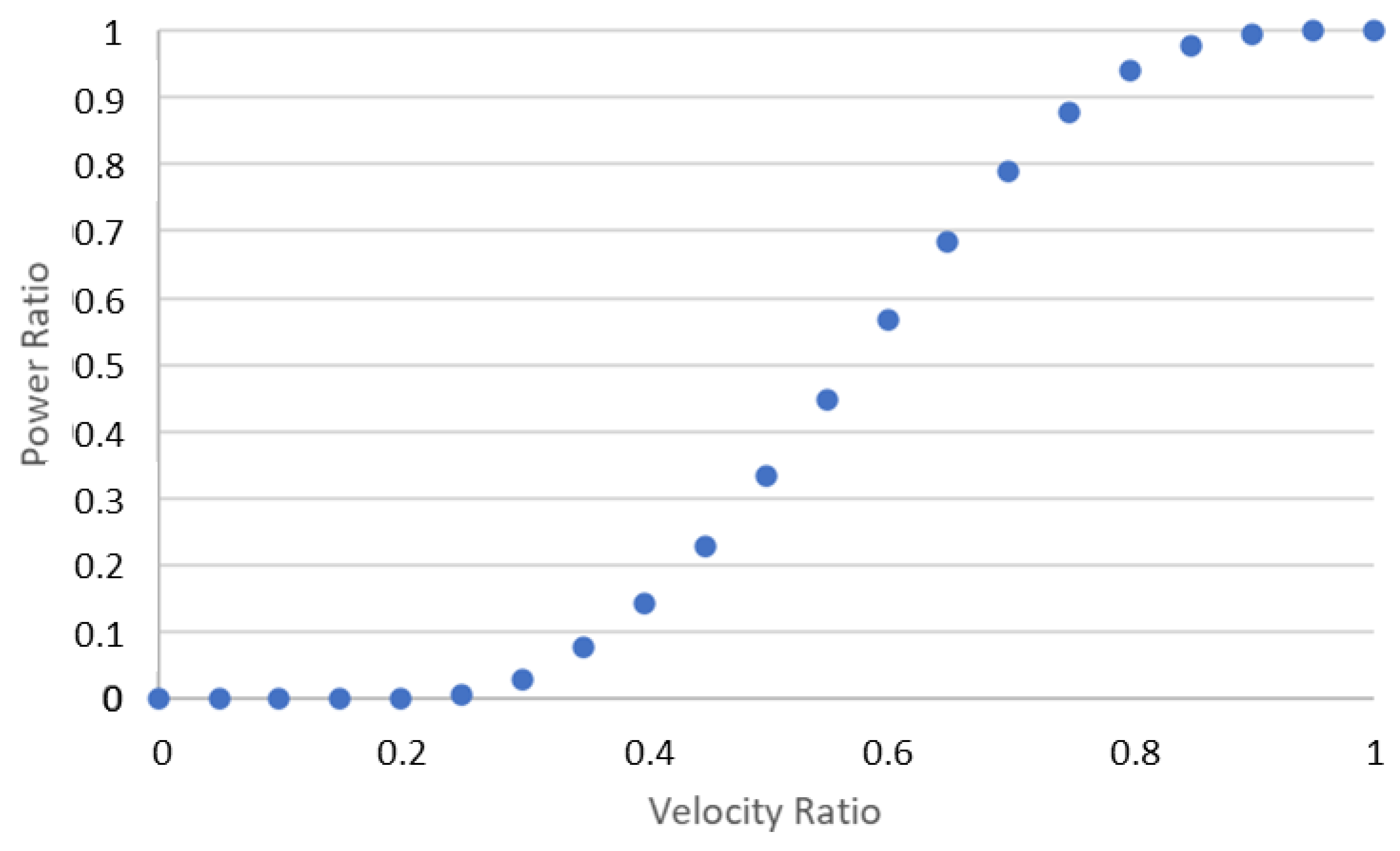
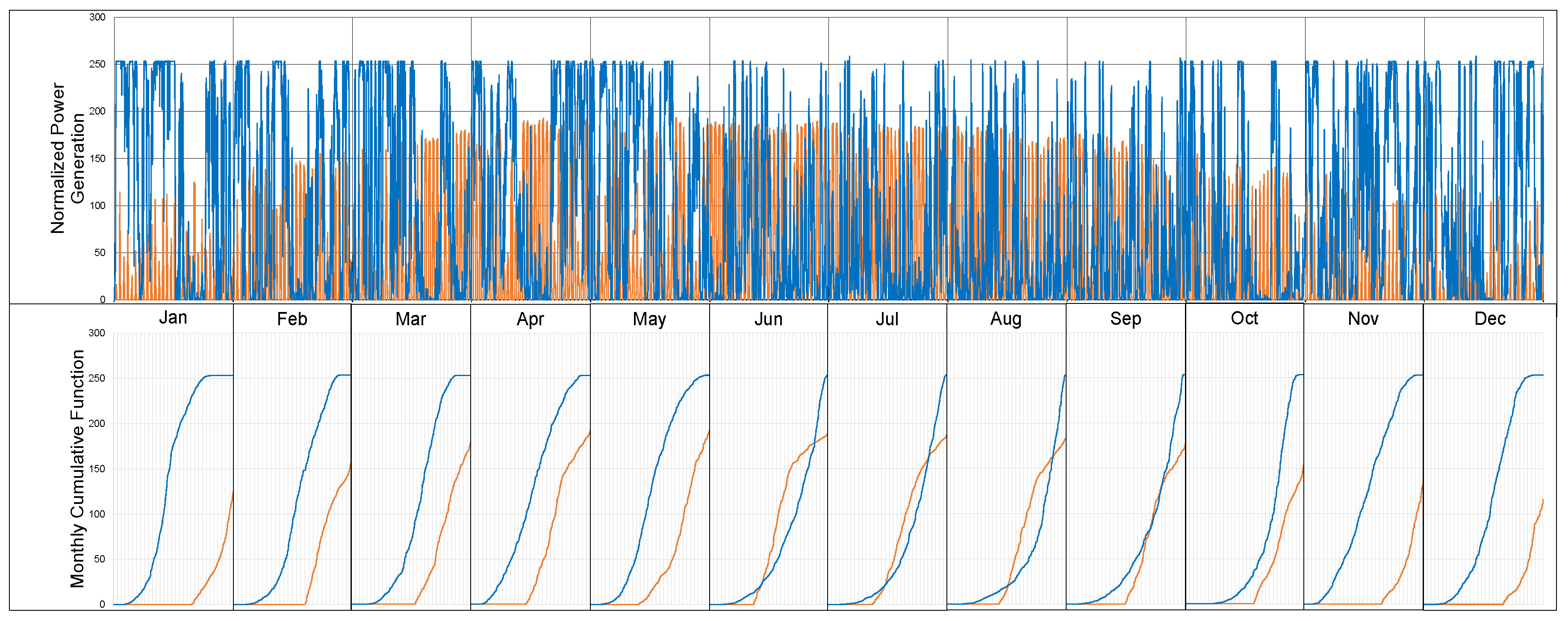


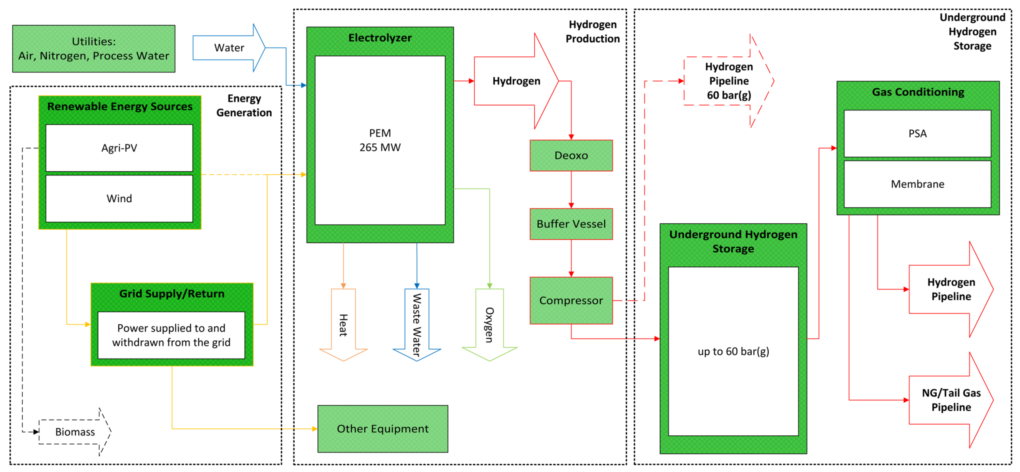

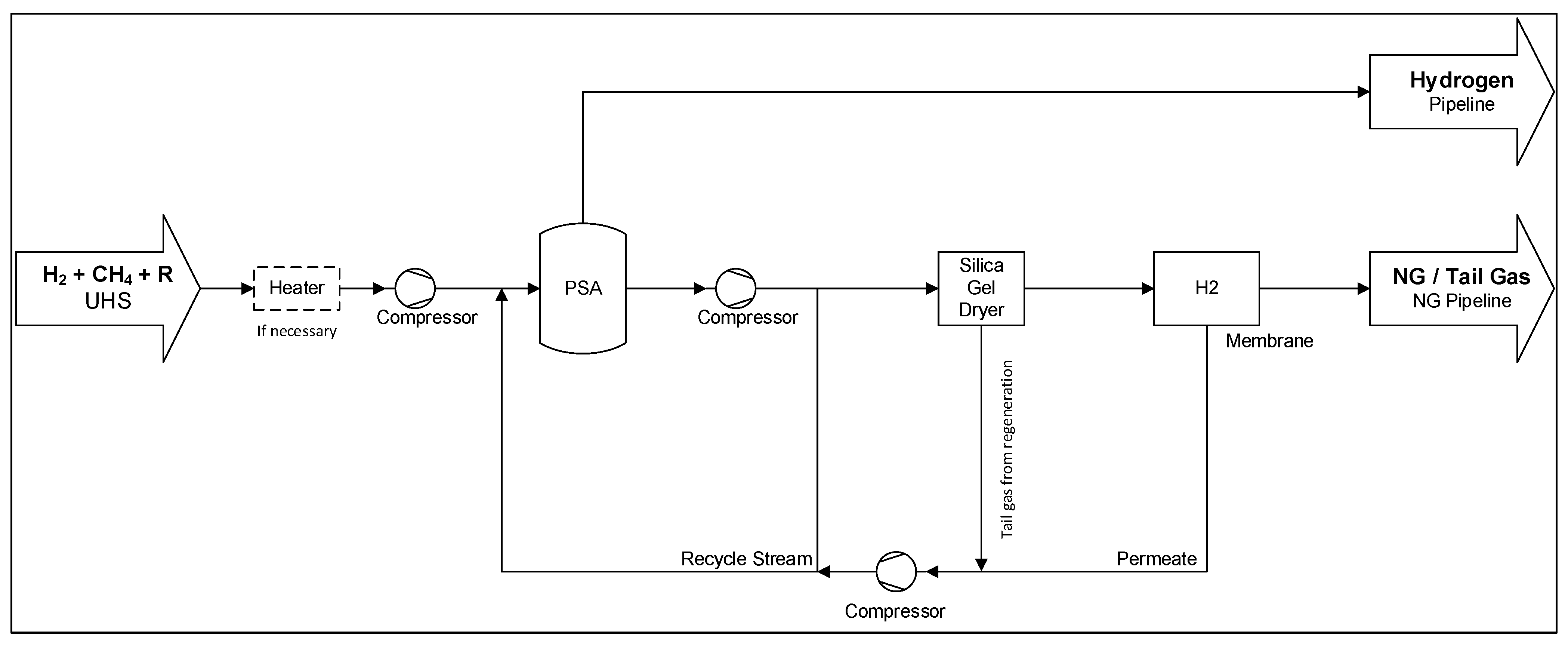
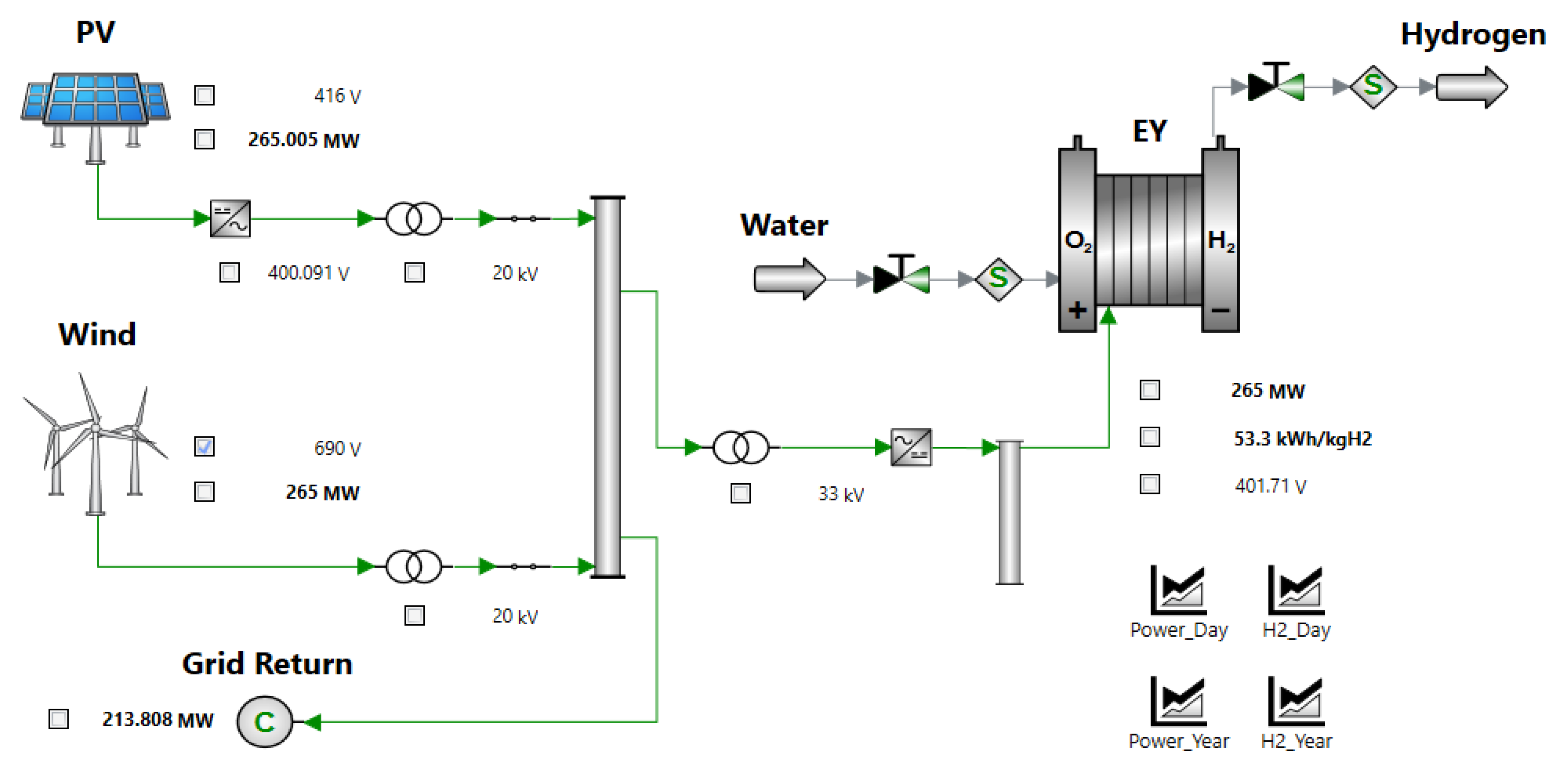
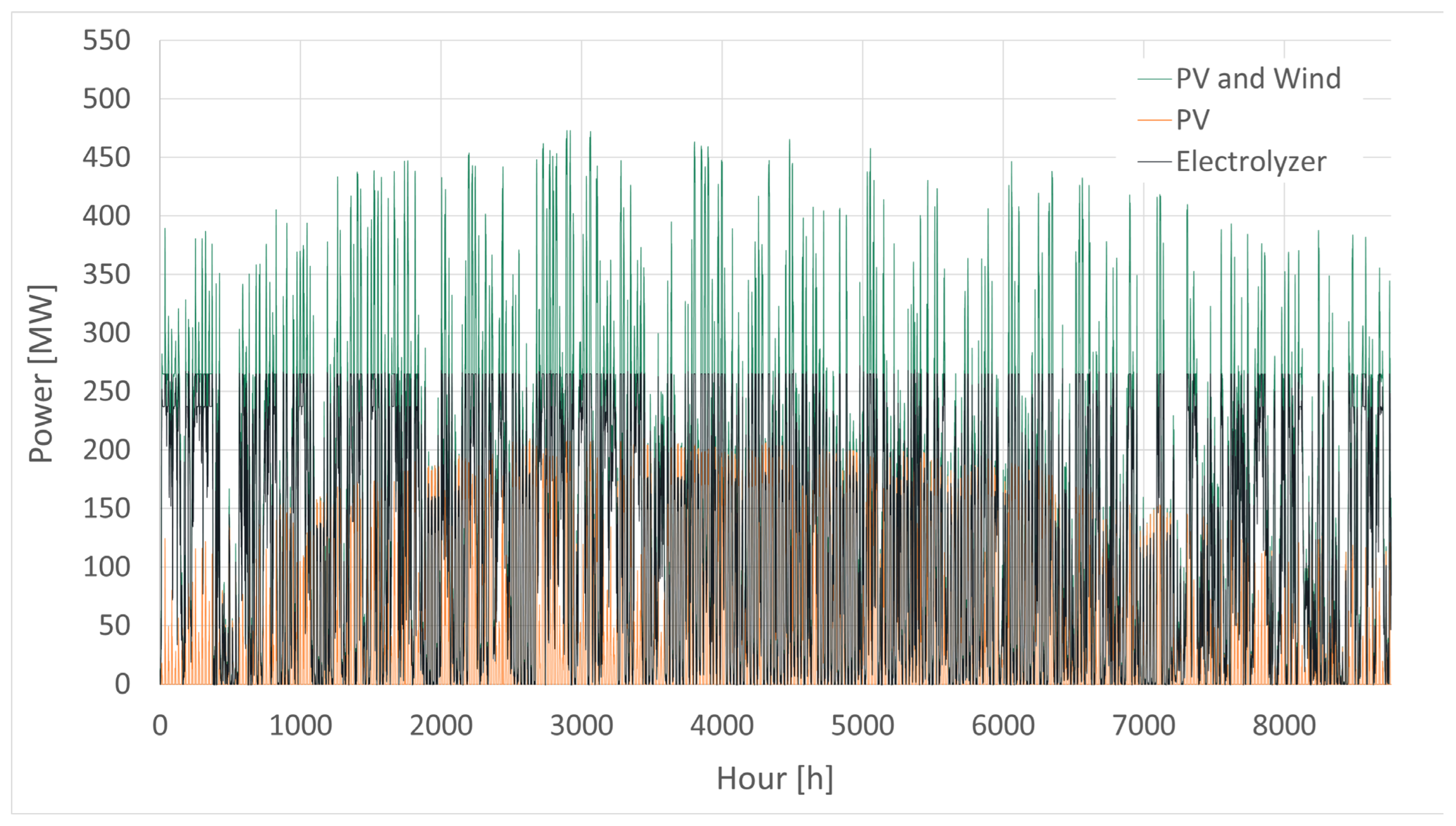
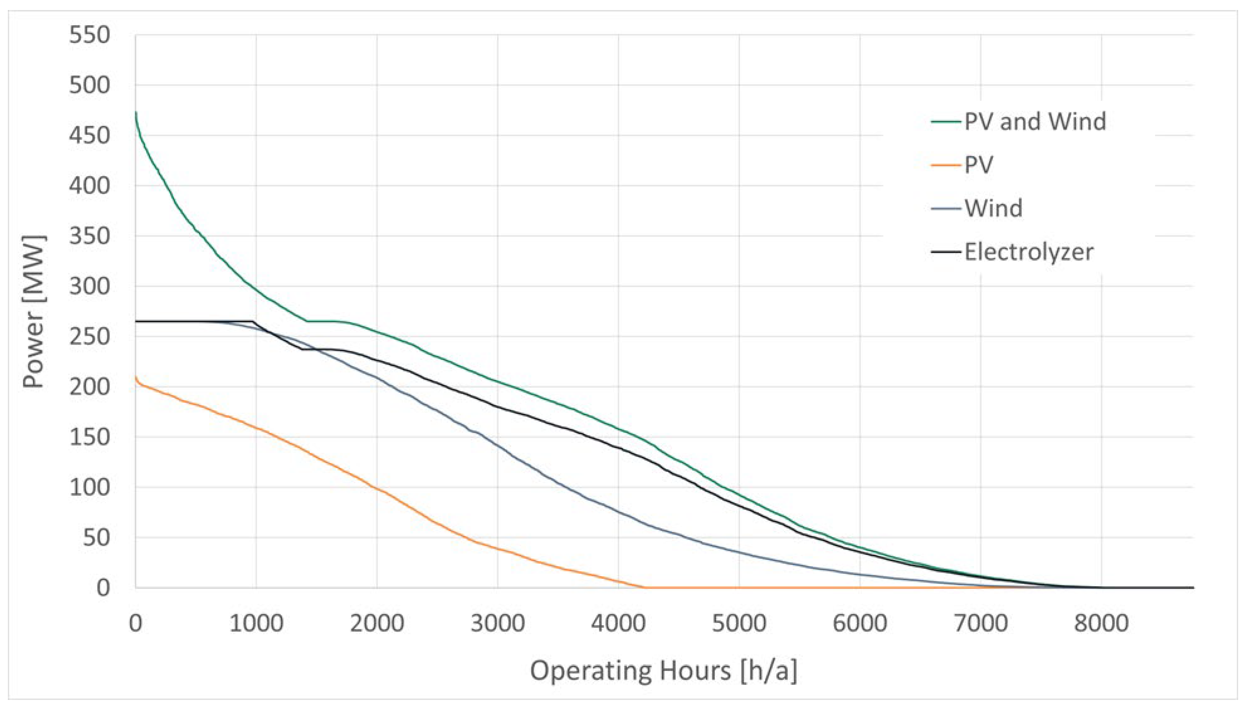

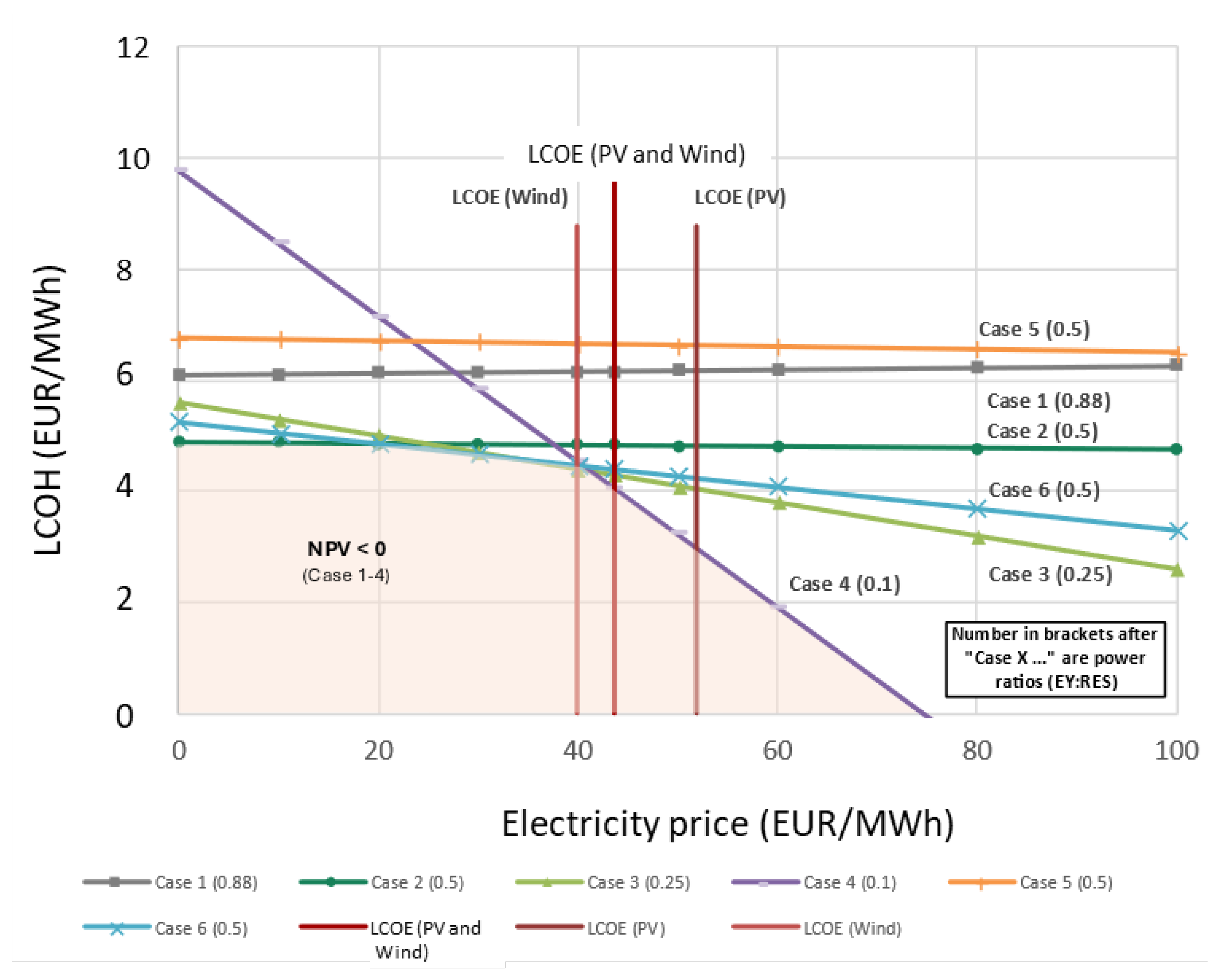
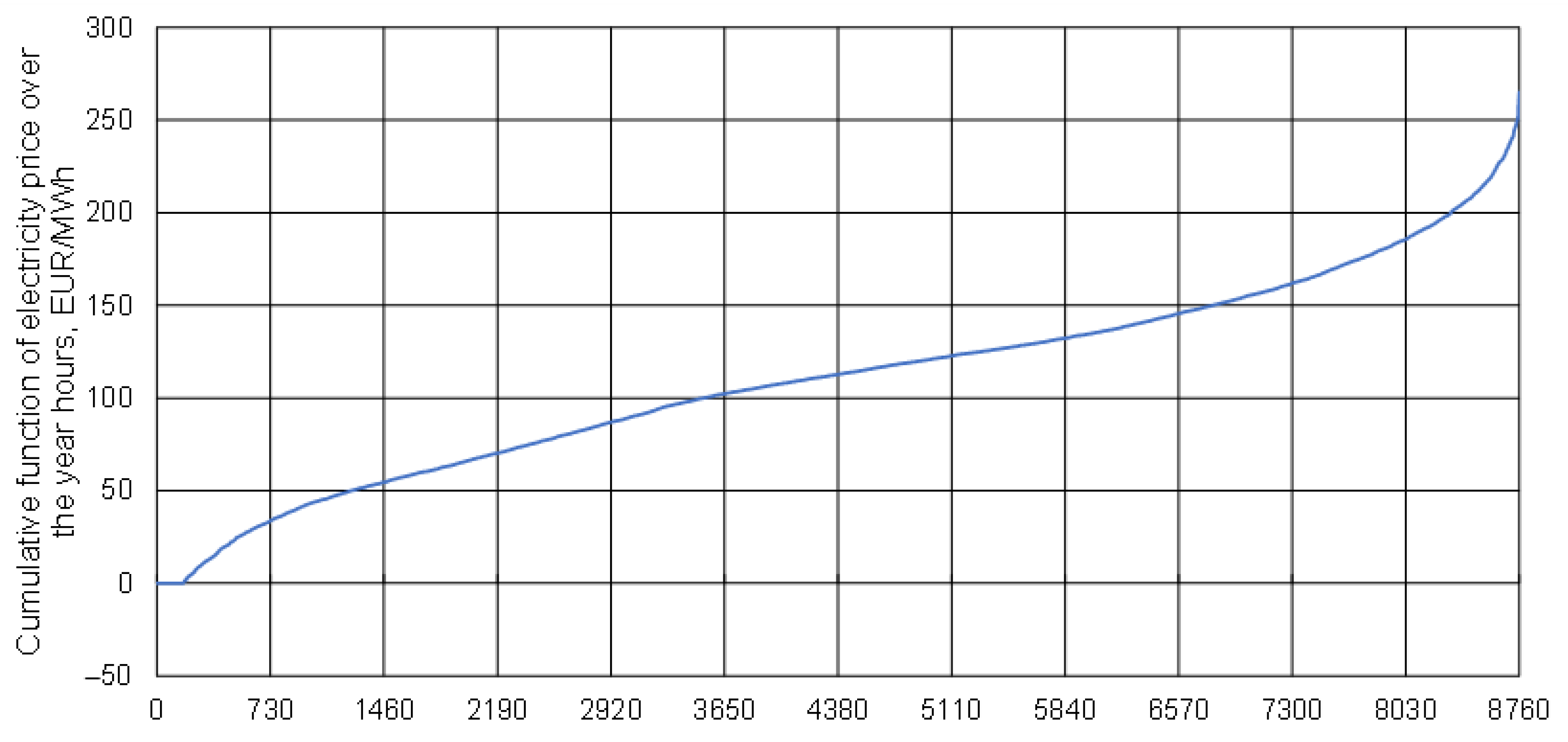
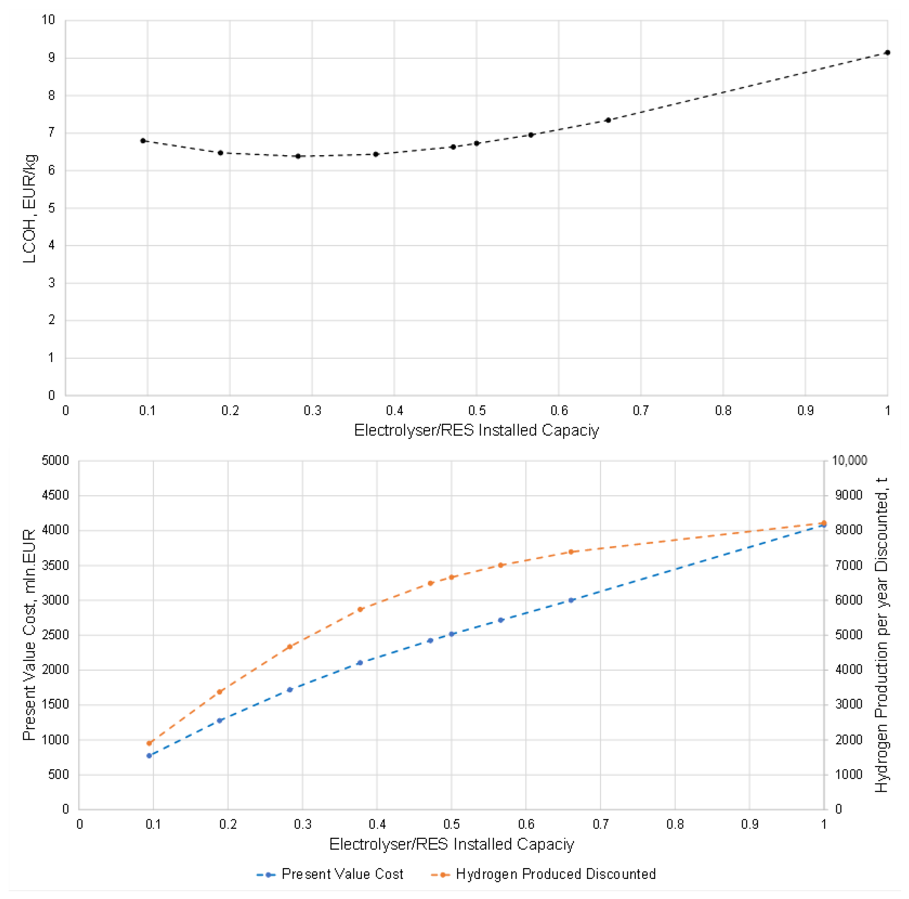
