Fault Diagnosis Method for Hydropower Station Measurement and Control System Based on ISSA-VMD and 1DCNN-BiLSTM

Abstract

Sudden failures of measurement and control circuits in hydropower plants may lead to unplanned shutdowns of generating units. Therefore, the diagnosis of hydropower station measurement and control system poses a great challenge. Existing fault diagnosis methods suffer from long fault identification time, inaccurate positioning, and low diagnostic efficiency. In order to improve the accuracy of fault diagnosis, this paper proposes a fault diagnosis method for hydropower station measurement and control system that combines variational modal decomposition (VMD), Pearson’s correlation coefficient, a one-dimensional convolutional neural network, and a bi-directional long and short-term memory network (1DCNN-BiLSTM). Firstly, the VMD parameters are optimised by the Improved Sparrow Search Algorithm (ISSA). Secondly, signal decomposition of the original fault signals is carried out by using ISSA-VMD, and meanwhile, the optimal intrinsic modal components (IMFs) are screened out by using Pearson’s correlation coefficient, and the optimal set of components is subjected to signal reconstruction in order to obtain the new signal sequences. Then, the 1DCNN-BiLSTM-based fault diagnosis model is proposed, which achieves accurate diagnosis of the faults of hydropower station measurement and control system. Finally, experimental verification reveals that, in comparison with other methods such as 1DCNN, BiLSTM, ELM, BP neural network, SVM, and DBN, the proposed approach in this paper achieves an exceptionally high average recognition accuracy of 99.8% in both simulation and example analysis. Additionally, it demonstrates faster convergence speed, indicating not only its superior diagnostic precision but also its high application value.

1. Introduction

In recent years, hydropower station measurement and control systems have become critical components in power generation control, playing an essential role in ensuring stable operations [1]. The occurrence of faults in these systems can lead to system failures, production interruptions, and significant economic losses [2]. Therefore, the ability to rapidly and accurately diagnose faults in the hydropower station measurement and control system is crucial for maintaining the stable operation of power systems. These systems are typically composed of multiple analog circuit boards that integrate power supply, signal acquisition, data processing, communication, and display functions. As the complexity of hydropower station measurement and control system increases, the difficulty of fault diagnosis also rises. Consequently, timely identification and localization of circuit faults within these systems are vital to prevent potential catastrophic outcomes [3].

Traditionally, fault diagnosis has relied on manual offline detection, which is complex and time-consuming. With the rapid advancement of artificial intelligence technologies, fault diagnosis in hydropower station measurement and control system has progressively shifted towards automated diagnosis, relying on the collection of system input and output signals, combined with feature extraction and classification algorithms. Fault diagnosis in hydropower station measurement and control system typically involves several key stages, including signal acquisition, signal decomposition, feature extraction, and fault classification. These systems employ sensors and data acquisition modules to monitor critical parameters such as voltage and current in real-time. When an abnormal event occurs during system operation, the system records fault signals. However, due to the nonlinear characteristics of hydropower station measurement and control system, these fault signals often exhibit non-stationary and nonlinear features [4], posing significant challenges for accurate diagnosis.

Signal decomposition and effective feature extraction from preprocessed fault signals are essential steps in fault diagnosis. Time-frequency domain analysis methods can jointly provide time and frequency information, making them highly valuable for comprehensive fault feature extraction. Methods such as wavelet packet decomposition [5], empirical mode decomposition (EMD) [6,7], synchrosqueezing wavelet transform (SWT) [8], and improved complete ensemble empirical mode decomposition with adaptive noise (ICEEMDAN) [9,10] have been widely applied for fault feature extraction. However, these approaches suffer from issues such as mode mixing or difficulty in selecting appropriate wavelet bases, limiting decomposition accuracy. Thus, choosing a suitable signal decomposition method is critical. To address these challenges, [10] proposed a finite sample fault diagnosis method based on signal feature extraction, and [7,11] introduced variational mode decomposition (VMD) for fault signal decomposition and extracted fault features using composite multiscale entropy. Compared to other methods, VMD demonstrates superior adaptive signal decomposition and feature extraction capabilities [12,13], achieving promising results in fault diagnosis. In recent years, the combination of VMD with other algorithms, such as fuzzy entropy [14] and multiscale fuzzy entropy [15], has shown significant performance improvements in motor bearing fault diagnosis. However, the effectiveness of VMD largely depends on parameter selection, which remains a key challenge in research. Traditional optimization algorithms, such as genetic algorithms (GA) [14], particle swarm optimization (PSO) [15], simulated annealing (SA) [16], and bat algorithms (BA) [17], have been applied to optimize VMD parameters, but they often suffer from local optima and unstable convergence, limiting further improvement in decomposition accuracy. To overcome this issue, the Sparrow Search Algorithm (SSA), a novel swarm intelligence optimization algorithm [18], has been introduced to optimize VMD parameters, owing to its superior convergence speed, stability, and robustness. However, SSA still faces challenges of local optima during the later iterations. Therefore, to enhance the efficiency and accuracy of VMD optimization for feature extraction in hydropower station measurement and control system, this paper proposes an improved Sparrow Search Algorithm (ISSA), incorporating Sine chaotic mapping and adaptive t-distribution.

In terms of fault classification and diagnosis, classification algorithms analyze fault features to determine the type and location of system faults. Traditional methods, such as BP neural networks [19], support vector machines (SVM) [20], and extreme learning machines (ELM) [21], have been widely used in fault diagnosis. More recently, deep learning algorithms, such as convolutional neural networks (CNN) [22], one-dimensional convolutional neural networks (1DCNN) [23], and bidirectional long short-term memory networks (BiLSTM) [24], have shown strong feature extraction capabilities when dealing with nonlinear fault signals. However, the application of these models in hydropower monitoring and control system fault diagnosis remains limited. The 1DCNN effectively extracts local features from fault signals, but it lacks the ability to handle sequential information, making it unable to address long-term dependencies. BiLSTM can resolve this issue, but its feature extraction capability is relatively weaker. Therefore, this paper combines the strengths of 1DCNN and BiLSTM by inputting spatial features extracted by 1DCNN into the BiLSTM network to enhance the accuracy of fault diagnosis in hydropower station measurement and control system [25].

This paper proposes to use ISSA-VMD to decompose the original fault signals and combine the Pearson correlation coefficient with the preferred IMF components to reconstruct the signal sequences, which are then inputted into a fault diagnosis model based on 1DCNN-BiLSTM to achieve the fault classification of hydropower station measurement and control system. The main contributions of this paper are as follows:

(1)

An improved Sparrow Search Algorithm (ISSA) is proposed, which incorporates Sine chaotic mapping and adaptive t-distribution to address the issues of local optima and premature convergence commonly encountered in traditional SSA.

(2)

The ISSA is employed to optimize the parameters of Variational Mode Decomposition (VMD), enhancing the decomposition accuracy. Additionally, the Pearson correlation coefficient is utilized to select intrinsic mode functions (IMFs), further improving the extraction and selection of fault signal features.

(3)

A fault classification method based on 1DCNN and BiLSTM is proposed, effectively extracting both spatial and temporal features of fault signals in hydropower station measurement and control system, significantly improving diagnostic accuracy.

The structure of this paper is organized as follows: Section 2 reviews the fundamental methods for signal decomposition and fault diagnosis, including the Sparrow Search Algorithm (SSA), Variational Mode Decomposition (VMD), 1D Convolutional Neural Networks (1DCNN), and Bidirectional Long Short-Term Memory (BiLSTM). Section 3 highlights the main contributions of this work, focusing on the proposed fault diagnosis method for hydropower station measurement and control systems based on ISSA-VMD and 1DCNN-BiLSTM. This section introduces the Improved Sparrow Search Algorithm (ISSA), its application in optimizing VMD, the combined 1DCNN-BiLSTM model, and the overall process of the proposed methodology. Section 4 provides experimental validation, including both simulation and case studies. Section 5 concludes the paper, summarizing the key findings and discussing the implications of the proposed method.

2. Theoretical Approach

2.1. Sparrow Search Algorithm

The Sparrow Search Algorithm (SSA) is a novel swarm intelligence optimization algorithm introduced by Jian Kai Xue and Bo Shen in 2020 [26]. In SSA, sparrow populations are categorized into two roles: discoverers and followers. Discoverers search for food and determine the direction of the food source for the entire population, while followers forage by following the direction provided by the discoverers.

In a sparrow population, discoverers and followers each make up a specific proportion of the group and adjust their positions based on their adaptation to the environment. The position update is governed by the following formula:

$$X_{i,j}^{t+1}=\left\{\begin{array}{l}{X}_{i,j}^t·\mathit{exp}\left(-{\displaystyle \frac{i}{\beta ·po{p}_m}}\right)\hspace{1em}if R_2<S_T\\ X_{i,j}^t+M·N\hspace{1em}\hspace{1em}\hspace{1em}\hspace{1em}if R_2\ge S_T\end{array}\right.$$

(1)

where: ${\mathit{pop}}_m$ is the maximum number of iterations, t is the current number of iterations, X_ij is the position of the ith sparrow in the jth dimension, β is a random number in the range of (0, 1], M is a random number obeying a normal distribution, N is a matrix of 1 row and d columns all of which are 1, $R_2\in [0, 1]$ is the early warning value of the risk of sparrow predation by the outside world, and $S_T\in [0.5, 1]$ is the safety value of the location position’s safety value.

When $R_2<S_T$, there is no risk of predation in the current foraging area; when $R_2>S_T$, all sparrows move as a whole to find a safe foraging area.

When the follower and the finder compete with each other, the sparrows re-update their position by the following equation:

$$X_{i,j}^{t+1}=\left\{\begin{array}{c}M·\mathit{exp}\left({\displaystyle \frac{X_w-X_{i,j}^t}{i^2}}\right)\hspace{1em}\hspace{1em}\hspace{1em}if i>{\displaystyle \frac{n}{2}}\hfill \\ X_p^{t+1}+\left|X_{i,j}^t-X_p^{t+1}\right|·A^{+}·N\hspace{1em}\mathrm{o}\mathrm{t}\mathrm{h}\mathrm{e}\mathrm{r}\mathrm{w}\mathrm{i}\mathrm{s}\mathrm{e}\end{array}\right.$$

(2)

where $X_w$ is the worst position the global is in, $X_p$ is the optimal position the finder is in the foraging region, A⁺ = A^T(AA^T)⁻¹, and A is a random 1 or −1 matrix of 1 row and d columns. When $i>n/2$, it indicates that the finder needs to travel to another area to re-forage.

Individuals with the ability to send early warning letters for other sparrows in a sparrow population make up 10–20% of the entire population.

$$X_{i,j}^{t+1}=\left\{\begin{array}{c}{X}_b^t+\xi \left|X_{i,j}^t-X_b^t\right|\hspace{1em}\hspace{1em}\hspace{1em}\hspace{1em}if\hspace{1em}{f}_i>f_g\\ X_{i,j}^t+J·\left({\displaystyle \frac{\left|X_{i,j}^t-X_w^t\right|}{(f_i-f_w)+\psi }}\right)\hspace{1em}if{f}_i=f_g\end{array}\right.$$

(3)

where: X_b is the global optimal position, ξ is the step parameter, $f_i$ is the individual fitness value of the sparrow, J is the random number in [−1, 1], ψ is the minimum constant, and $f_g$ and $f_w$ are the highest and lowest fitness values in the population. When $f_i>f_g$, sparrows are susceptible to predation; when $f_i=f_g$, some sparrows are aware of the danger in order to travel to a safe area and reduce predator attacks.

2.2. Variational Modal Decomposition Algorithm

Variational Mode Decomposition (VMD), proposed by Konstantin Dragomiretskiy and Dominique Zosso in 2014, can effectively solve the problems of endpoint effects and mode aliasing in EMD [7,27]. The algorithm consists of two main parts: constructing the variational problem and solving the variational problem.

(1)

Construction of variational problems

The constrained variational problem when VMD performs a K-order modal decomposition of a sequence signal is expressed as follows:

$$\begin{array}{l}\mathit{min}\left\{{\displaystyle \sum _{k=1}^K}{‖\mathsf{\partial }\left(t\right)\left[\left(\delta \left(t\right)+{\displaystyle \frac{j}{\pi t}}\right)\ast u_k\left(t\right)\right]e^{-j{\omega }_{k}t}‖}_2^2\right\}\\ s.t.\sum _{k=1}^K{u}_k=f\left(t\right)\end{array}$$

(4)

where: $f\left(t\right)$ represents the original sequence signal, $u_k$ and ${\omega }_k$ represent the modal function and centre frequency corresponding to the Kth IMF, respectively.

(2)

Solution of the variational problem

Introducing the augmented Lagrangian function for solving and transforming the constrained variational problem into an unconstrained variational problem.

$$\begin{array}{cc}\hfill L\left(\left\{u_k\right\},\left\{{\omega }_k\right\},\lambda \right)& ={‖f\left(t\right)-\sum _{k=1}^K{u}_k\left(t\right)‖}_2^2\hfill \\ & +\alpha {\sum _{k=1}^K‖{\partial }_t\left[\left(\delta \left(t\right)+{\displaystyle \frac{j}{\pi t}}\right)\ast u_k\left(t\right)\right]e^{-j{\omega }_{k}t}‖}_2^2\hfill \\ & +⟨\lambda \left(t\right),f\left(t\right)-\sum _{k=1}^K{u}_k\left(t\right)⟩\hfill \end{array}$$

(5)

where: λ is the Lagrange multiplier operator and α penalty factor.

The optimal solution of Equations (6) and (7) is solved using the alternating multiplier method and the results are shown below.

$${\widehat{u}}_k^{n+1}\left(\omega \right)={\displaystyle \frac{\widehat{f}\left(\omega \right)-{\sum }_{i<k}{\widehat{u}}_k^{n+1}\left(\omega \right)-{\sum }_{i>k}{\widehat{u}}_k^{n+1}\left(\omega \right)+\frac{{\widehat{\lambda }}^n\left(\omega \right)}{2}}{1+2\alpha {\left(\omega -{\omega }_k^n\right)}^2}}$$

(6)

$${\omega }_k^{n+1}={\displaystyle \frac{{\int }_0^{\infty }\omega {\left|{\widehat{u}}_k^{n+1}\left(\omega \right)\right|}^{2}d\omega }{{\int }_0^{\infty }{\left|{\widehat{u}}_k^{n+1}\left(\omega \right)\right|}^{2}d\omega }}$$

(7)

$${\widehat{\lambda }}^{n+1}\left(\omega \right)={\widehat{\lambda }}^n\left(\omega \right)+\tau \left(\widehat{f}\left(\omega \right)-\sum _k\left|{\widehat{u}}_k^{n+1}\left(\omega \right)\right|\right)$$

(8)

where: τ is the update parameter of VMD, n is the number of iterations until convergence.

Before using the VMD for signal decomposition, it is necessary to confirm the relevant parameters in the VMD in advance, when the convergence conditions of the algorithm are met Equation (11) and the discriminant accuracy ε > 0, the VMD algorithm reaches the convergence requirements and stops iterating; otherwise, it returns to continue the decomposition.

$${\displaystyle \sum _{k=1}^K}{‖{\widehat{u}}_k^{n+1}-{\widehat{u}}_k^n‖}_2^2/{‖{\widehat{u}}_k^n‖}_2^2<\epsilon$$

(9)

2.3. One-Dimensional Convolutional Neural Networks

The structure of a one-dimensional convolutional neural network (1DCNN) mainly consists of an input layer, a convolutional layer, a pooling and fully connected layer, and an output layer [28].

The role of the convolutional layer is to perform feature extraction on the input signal and its operational expression is:

$$X_j^l=f\left({\sum }_{i\in M_j}{X}_i^{l-1}{W}_{ij}^l+b_j\right)$$

(10)

where: f is the activation function; $M_j$ is the operation of the input; l is the length of the input; $X_i^{l-1}$ is the region of the target input to be convolved; $W_{ij}^l$ is the convolution kernel, also known as the weights; and $b_j$ is the bias coefficient of the corresponding convolution kernel.

The role of the pooling layer is to downsample the feature sequence data extracted from the convolutional layer to prevent overfitting from occurring by reducing the amount of data computation in the neural network. Maximum pooling is usually used for downsampling, and the operational expression for maximum pooling is:

$$y_i^l=maxpooling\left(x_j^l,scale,stride\right)$$

(11)

where: $y_i^l$ is the output of the neuron in the current layer; $maxpooling$ is the downsampling function, which is taken as the maximum value; scale is the size of pooling; and stride is the number of pooling steps.

The role of the fully connected layer is to integrate the features extracted from the convolutional and pooling layers to achieve accurate recognition of the detection target. At the same time the fully connected layer can transform the multidimensional input into a one-dimensional output to get the final classification result.

The output layer usually uses softmax classifier to output classification labels.

2.4. Bidirectional Long and Short-Term Memory Network Theory

BiLSTM model is composed of both forward and reverse LSTM models and is a kind of Bidirectional Recurrent Neural Network (BiRNN), thus taking full advantage of both to deal with the problem [29].

Both forward and reverse are connected to the output layer, which can obtain the information of each moment of sequence data forward and reverse in the hidden layer, and the state update formulas of its forward and reverse LSTM hidden layers are as follows, respectively:

$$h_t^{+}=LST{M}^{+}\left(h_{t-1},x_t\right)$$

(12)

$$h_t^{-}=LST{M}^{-}\left(h_{t-1},x_t\right)$$

(13)

where $h_t^{+}$ and $h_t^{-}$ are the states of the forward and reverse LSTM hidden layers at moment t, respectively.

Combining the outputs of the forward and reverse LSTMs and feeding them into the output layer, the formula for the output state is

$$O_t={\omega }^{+}{h}_t^{+}+{\omega }^{-}{h}_t^{-}+b_o$$

(14)

where: ω+, ω+ are the values of the weights of the forward and reverse LSTMs, respectively, and $b_o$ is the value of the bias of the BiLSTM output.

Among models of the same type, BiLSTM is particularly effective at processing time series data because it can analyze sequences in both forward and reverse directions. Given that the voltage signals collected in analog circuits are periodic and exhibit strong correlations within the sequences, the BiLSTM model is an ideal choice for fault classification in this context.

3. Fault Diagnosis of Hydropower Station Measurement and Control System Based on ISSA-VMD and 1DCNN-BiLSTM

3.1. Improvement of the Sparrow Search Algorithm

3.1.1. Sine Chaotic Mapping

When applying SSA to optimization problems, population initialization may lead to an uneven distribution of the population, and in the later stages of the iteration, it appears that the diversity of the population becomes less, which causes the algorithm to easily fall into a local optimal solution or converge prematurely.

According to the literature [30], Sine chaotic mapping is more capable of producing a uniform distribution than Logistic and Tent chaotic mapping. Therefore, in this paper, Sine chaotic mapping is introduced to initialize the sparrow population in order to improve the uniformity of the distribution of the sparrow population in the search space and the ability of global search, and to avoid SSA falling into a local optimal solution. Its expression is as follows:

$$x_{k+1}={\displaystyle \frac{\beta }{4}}\mathit{sin}\left(\pi x_k\right),\beta \in \left(0,\left.4\right]\right.$$

(15)

where: x_k is the iterative sequence value and k takes a non-negative integer.

3.1.2. Adaptive t-Distribution

The t-distribution was proposed by Gosset in 1908 [11] and its probability density function has the following expression:

$$f\left(x\right)={\displaystyle \frac{\Gamma \left(\frac{m+1}{2}\right)}{\sqrt{m·\pi }·\Gamma \left(\frac{m}{2}\right)}}{\left(1+{\displaystyle \frac{x^2}{m}}\right)}^{-\left(m+1\right)/2}$$

(16)

where: m is the parameter degrees of freedom of the t-distribution.

In order to improve the ability of SSA to jump out of the local optimum at the later stage of iteration, an adaptive t-distribution [31] is introduced to update the position of the sparrow with a perturbation variant at the optimal solution.

$$x_i^{\ast }=x_i^k+x_i^k·t\left(iter\right)$$

(17)

where: $x_i^{\ast }$ is the latest position that the sparrow is in after adaptive mutation; $x_i^k$ is the updated position of the sparrow after the kth iteration; where $x_i^k·t\left(\mathit{iter}\right)$ is the added random disturbance term, and t(iter) is the parameter degree of freedom of the adaptive t-distribution in terms of the number of algorithm iterations.

Define the probability of adaptive t-distribution mutation as P. After performing the mutation operation, the mutated individual is compared with the original individual, and the position at the time of highest fitness is selected as the latest position of the current sparrow individual

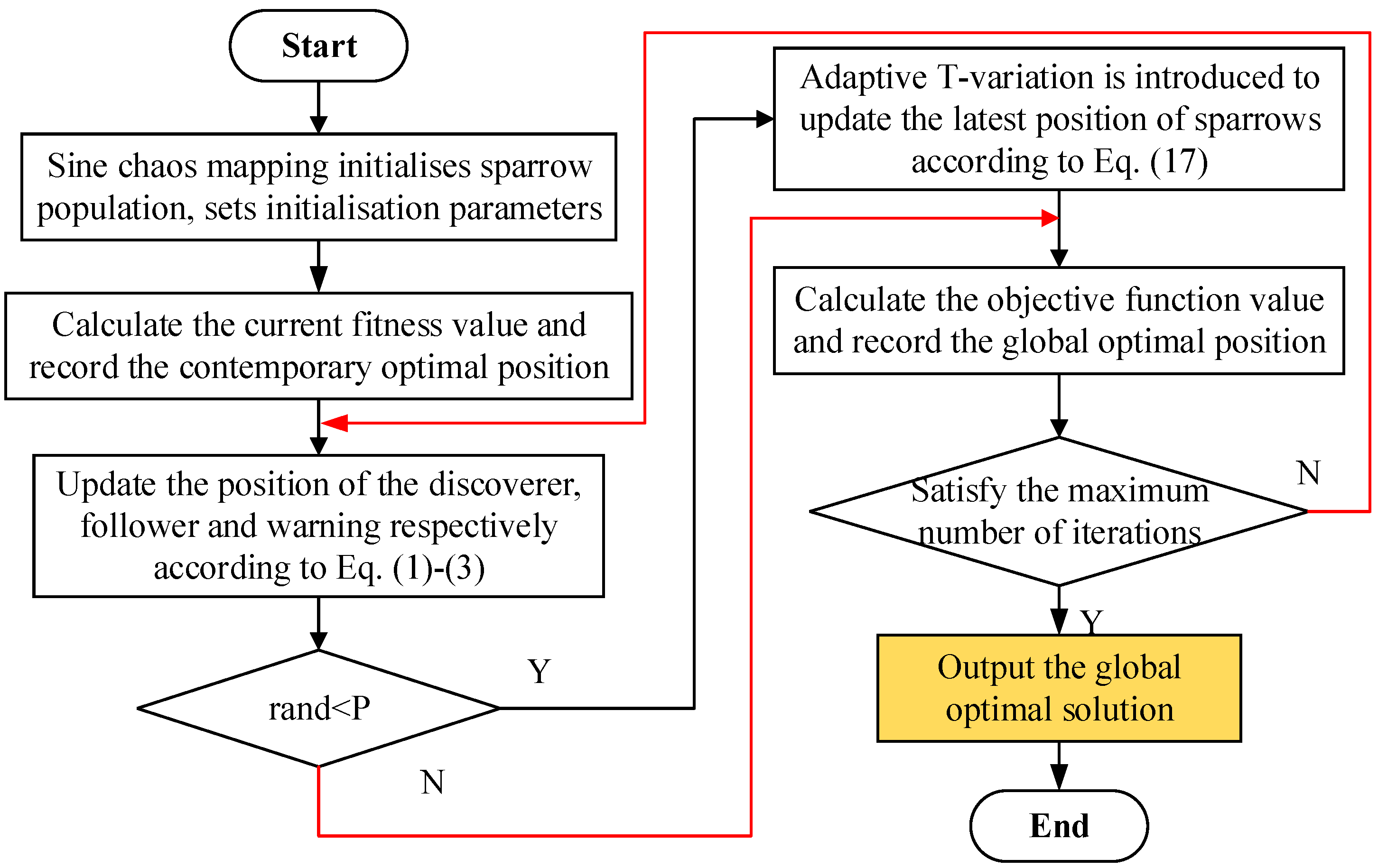
3.1.3. Improvement of the Flow of the Sparrow Search Algorithm

When addressing optimization problems with SSA, the algorithm may suffer from premature convergence during the later stages of iteration due to reduced population diversity, making it susceptible to getting trapped in local optima. To overcome this limitation, this paper proposes the introduction of Sine chaotic mapping and adaptive t-variation to develop an Improved Sparrow Search Algorithm (ISSA). These enhancements aim to boost the algorithm’s convergence speed and global optimization capability. The flowchart of the Improved Sparrow Search Algorithm is illustrated in Figure 1.

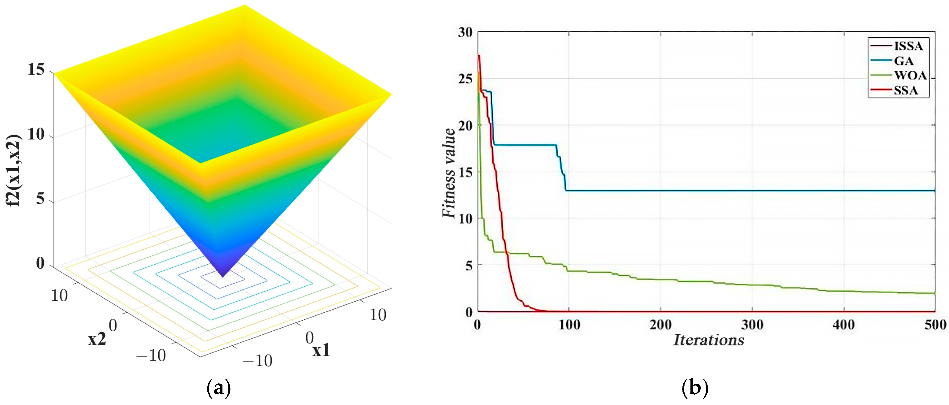
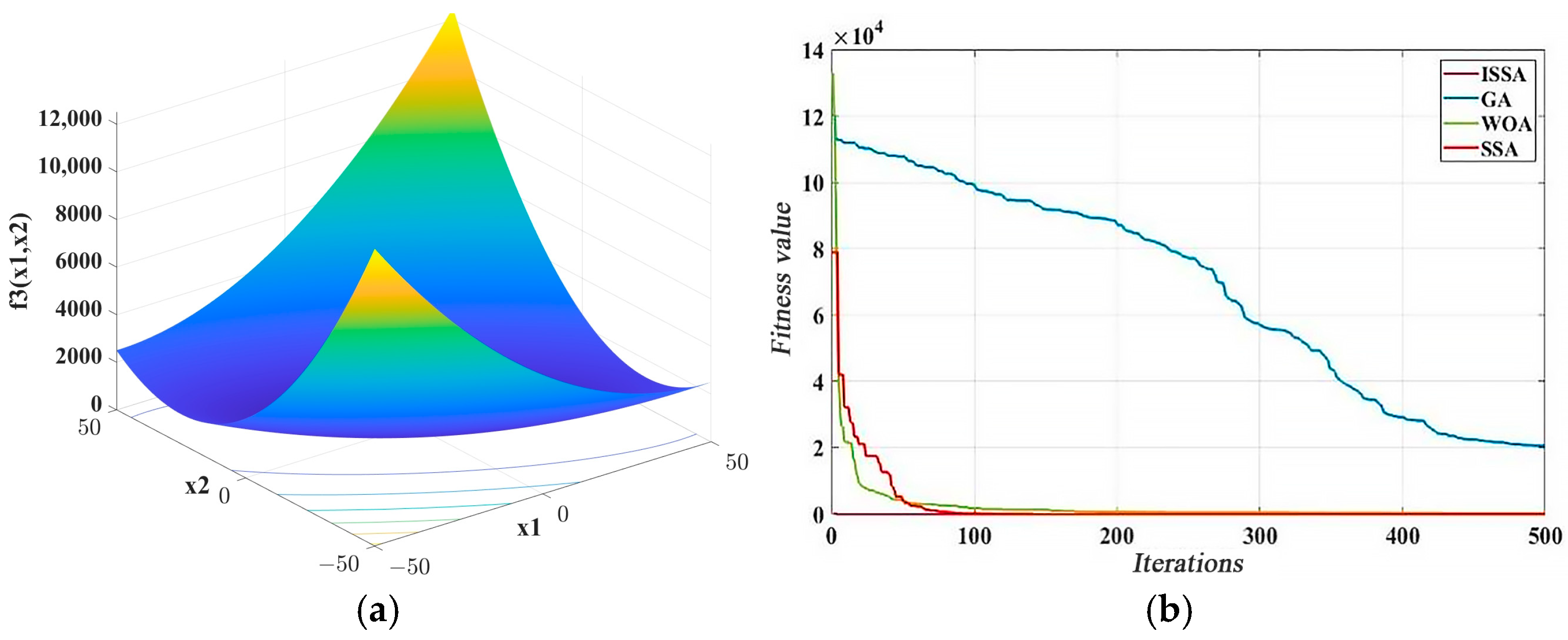
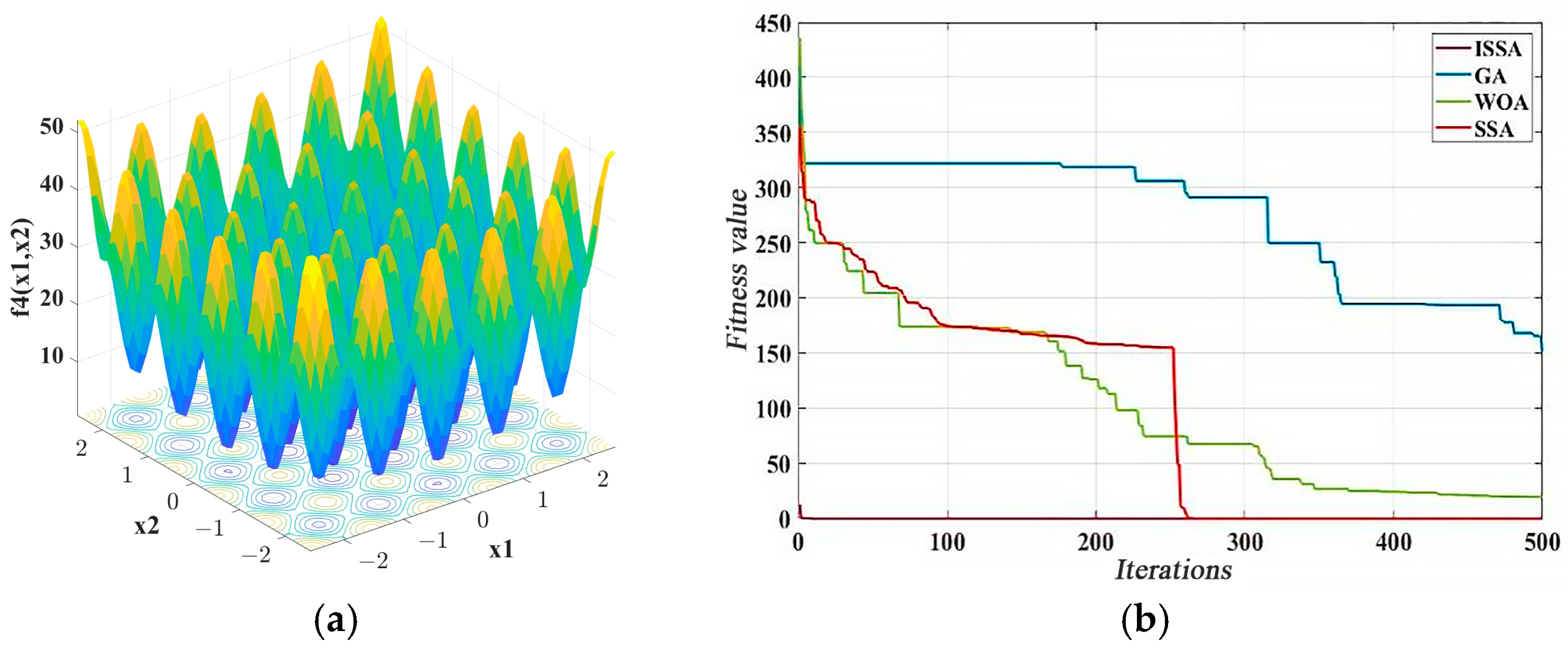
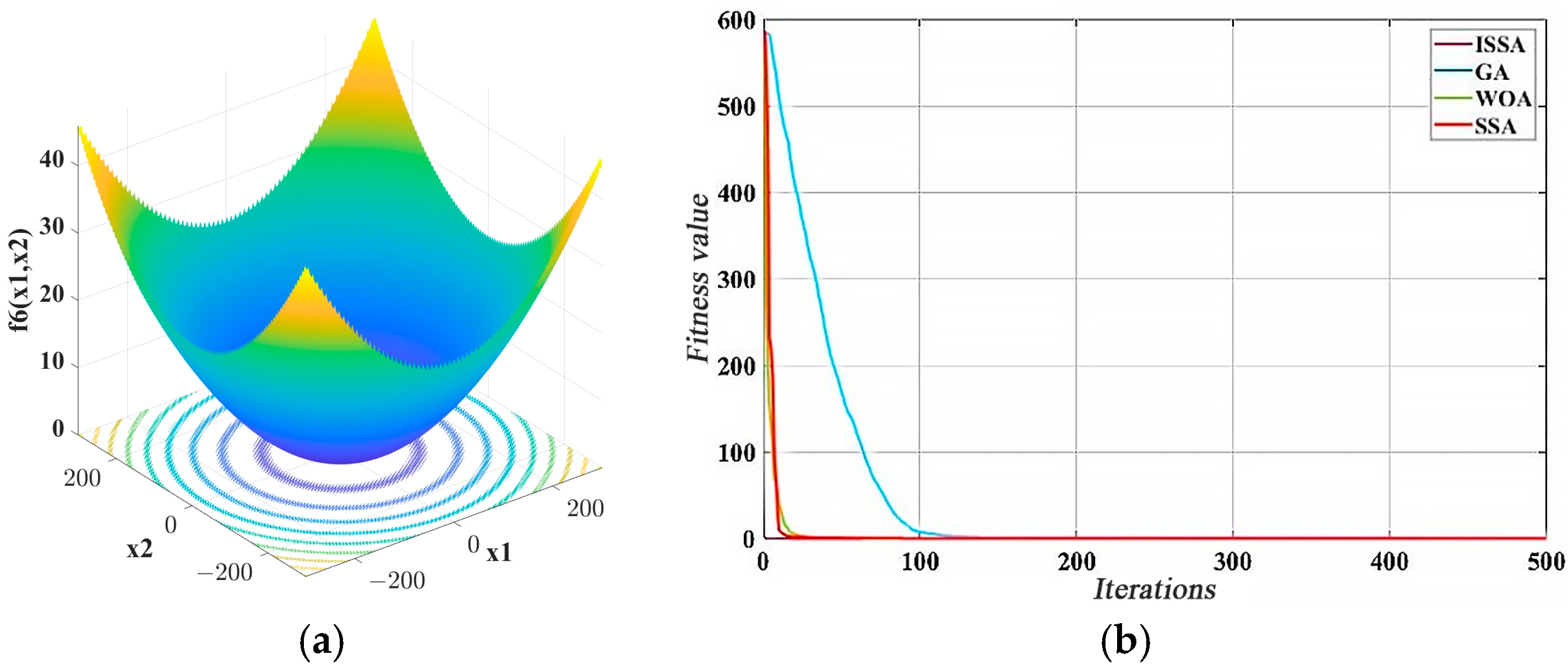
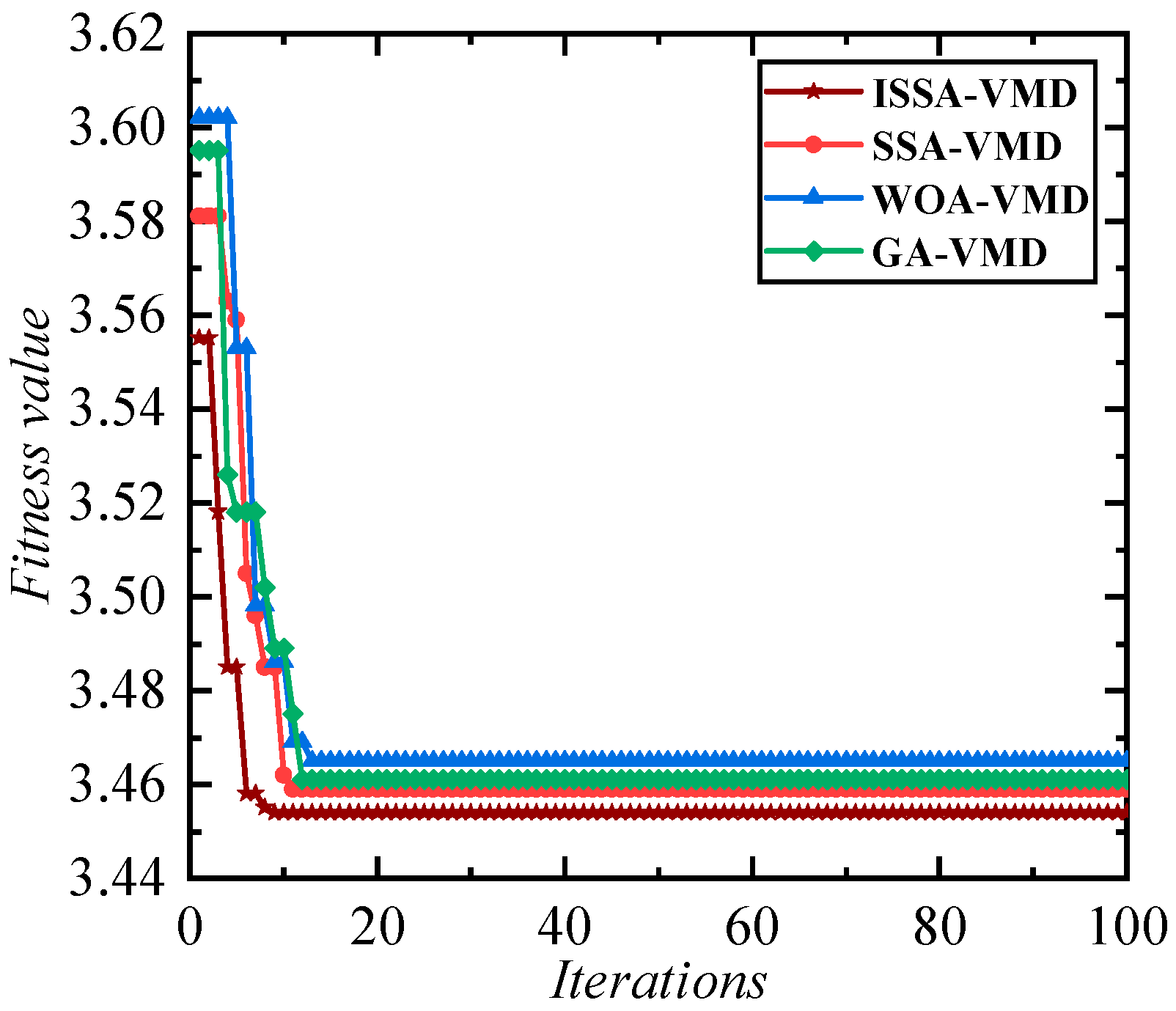
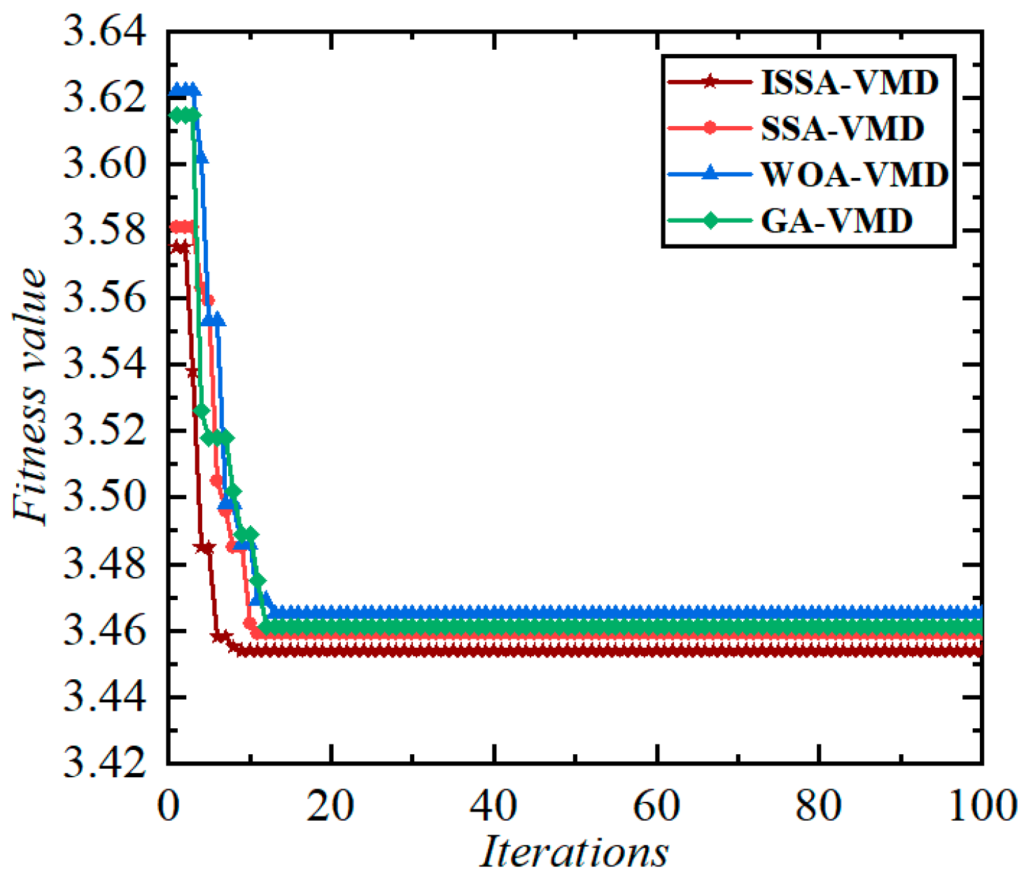
3.1.4. ISSA Performance Tests and Comparative Analyses

In order to verify the performance of ISSA, six benchmark test functions are selected to verify the convergence speed, global optimization ability and the ability to jump out of the local optimum of the algorithm. The basic information of the six benchmark test functions is shown in

Table 1. Information on the benchmarking function.

Type	Function Expression	Dimension	Scope of the Search for Excellence	Minimum Value
single peak function	$f_1\left(x\right)={\displaystyle \sum _{i=1}^n}{x}_i^2$	30	[−100, 100]	0
	$f_2\left(x\right)={\mathit{max}}_i\{\left|x_i\right|,1\le i\le n\}$	30	[−100, 100]	0
	$f_3\left(x\right)={{\displaystyle \sum _{i=1}^n}\left({\displaystyle \sum _{j=1}^i}{x}_j\right)}^2$	30	[−100, 100]	0
multimax multifunction	$f_4\left(x\right)={\displaystyle \sum _{i=1}^n}\left[x_i^2-10\mathit{cos}\left(2\pi x_i\right)+10\right]$	30	[−5.12, 5.12]	0
	$\begin{array}{ll}{f}_5\left(x\right)& =-20\mathit{exp}\left(-0.2\sqrt{{\displaystyle \frac{1}{n}}{\displaystyle \sum _{i=1}^n}{x}_i^2}\right)\\ & -\mathit{exp}\left({\displaystyle \frac{1}{n}}{\displaystyle \sum _{i=1}^n}\mathit{cos}\left(2\pi x_i\right)\right)+20+e\end{array}$	30	[−32, 32]	0
	$f_6\left(x\right)={\displaystyle \frac{1}{4000}}{\displaystyle \sum _{i=1}^n}{x}_i^2-{\displaystyle \prod ^{\stackrel{i=1}{n}}}\mathit{cos}\left({\displaystyle \frac{x_i}{\sqrt{i}}}\right)+1$	30	[−600, 600]	0

.

In order to accurately verify the performance of the ISSA algorithm, the dimensions of the test functions are all set to 30. According to the literature [7], the relevant parameter settings are carried out. The parameter settings of ISSA and SSA, Whale Optimization Algorithm (WOA), Genetic Algorithm (GA) are shown in

Table 2. Parameter settings of the optimization algorithm.

Algorithm Type	Parameterisation
ISSA	itermax = 500, Num = 50, ST = 0.8, PD = 0.7, SD = 0.2, P = 0.5
SSA	itermax = 500, Num = 50, ST = 0.8, PD = 0.7, SD = 0.2
WOA	itermax = 500, Num = 50
GA	itermax = 500, Num = 50, pc = 0.8, pm = 0.05, γ = 0.01

.

Table 3. Results of the mean and standard deviation of the four optimization algorithms.

Function	Norm	ISSA	SSA	WOA	GA
f1	Mean	5.07 × 10−140	5.63 × 10−84	7.15 × 10−34	1.72
	Standard deviation	2.728 × 10−139	2.42136 × 10−83	1.99205 × 10−33	0.702024047
f2	Mean	1.15 × 10−59	6.16 × 10−9	1.79	14.8
	Standard deviation	6.2091 × 10−59	5.19 × 10−9	0.222106	16.14894
f3	Mean	5.87 × 10−91	3.81 × 10−8	132	2.84 × 104
	Standard deviation	2.84527 × 10−90	1.05 × 10−7	51.02719	7877.528
f4	Mean	0.00	0.00	19.1	153
	Standard deviation	0.00	0.00	9.176026	29.31647
f5	Mean	4.44 × 10−16	3.16 × 10−6	2.38 × 10−7	2.17
	Standard deviation	1.97215 × 10−31	4.6892 × 10−18	3.6469 × 10−13	0.703959075
f6	Mean	0.00	8.45 × 10−3	5.92 × 10−3	8.46 × 10−2
	Standard deviation	0.00	0.032154	0.010103	0.031793

shows that the average result of ISSA is closest to the theoretical value of 0, indicating that ISSA has the highest optimization accuracy among the four algorithms, significantly enhancing the performance of SSA. Additionally, ISSA demonstrates the smallest standard deviation in the optimization results, reflecting its high stability. In five out of the six test functions, SSA’s standard deviation is second only to that of ISSA. Although ISSA does not achieve the smallest standard deviation in the f6 test function, it still outperforms the other three algorithms, further highlighting its ability to enhance the stability of SSA.

In order to observe more clearly the iterative optimization convergence process of ISSA, SSA, WOA, and GA algorithms, and to comprehensively compare the convergence speed of the four algorithms, the relationship between the fitness value of the test function and the number of iterations, this paper plots the iterative convergence curves of the optimization algorithms to better reveal the ability of each algorithm to globally find an optimal solution. Specifically, the iterative optimization convergence curves of the four optimization algorithms in the six test functions are shown in Figure 2, Figure 3, Figure 4, Figure 5, Figure 6 and Figure 7, respectively.

After the completion of the algorithm iteration, the mean and standard deviation of the objective function are selected as evaluation indexes to measure the performance of the algorithm, and the specific results are shown in Table 3.

Figure 2, Figure 3, Figure 4, Figure 5, Figure 6 and Figure 7 illustrate that during the solving process of various benchmark test functions, ISSA demonstrates a significantly faster iterative convergence speed compared to SSA, WOA, and GA algorithms, achieving lower adaptation values, which suggests higher optimization accuracy. When solving functions f2 and f4, WOA and GA tend to get trapped in local optima, while SSA converges after 84 and 268 iterations, respectively. In contrast, ISSA converges in fewer than 10 iterations, highlighting its ability to enhance the convergence speed of SSA.

A comprehensive analysis of the six test functions reveals that ISSA outperforms SSA, WOA, and GA in terms of optimization accuracy, convergence speed, and global optimization capability. Moreover, ISSA exhibits superior algorithmic stability, indicating that it not only improves the convergence speed of SSA but also effectively addresses the issue of premature convergence to local optima.

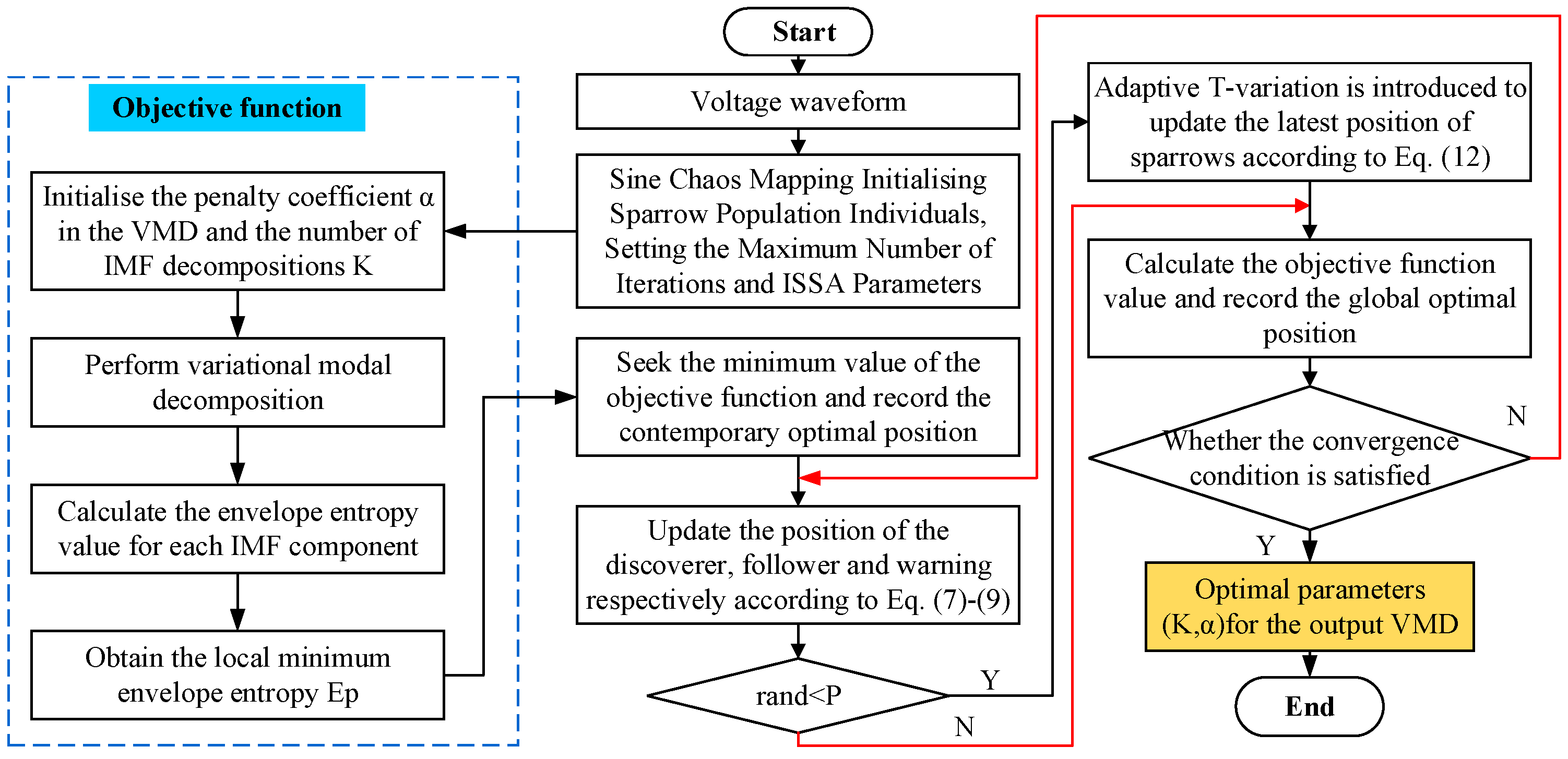
3.2. ISSA Optimization of the VMD Process

In the process of signal decomposition using VMD, the values of the number of IMF components, K, and the quadratic penalty factor, α, have a large impact on the signal decomposition results. In addition to K and α, the parameters such as convergence tolerance, noise tolerance τ, DC component, and initialization value in it have less influence on the decomposition results, and they are all set to the initial values. Therefore, before using VMD for signal decomposition, it is necessary to choose appropriate K and α.

When ISSA is used to optimize the parameters of the VMD, the envelope entropy Ep is selected as the fitness function, and the whole search process is to seek the optimal parameter combination [K, α] corresponding to the local minimum envelope entropy. Therefore, the constructed fitness function ${\mathrm{f}}_{\mathit{fitness}}$ is:

$$f_{fitness}=E_p$$

(18)

The expression for the envelope entropy E_p in E_q:

$$\left\{\begin{array}{l}{e}_j=a\left(j\right)/{\sum }_{j=1}^{n}a\left(j\right)\\ E_p=-{\sum }_{j=1}^n{e}_j\mathit{lg}{e}_j\hfill \end{array}\right.$$

(19)

where: j = 1, 2, 3, …, n; a(j) is the envelope signal of the IMF component and e_j is obtained by normalizing a(j).

When ISSA is used to optimize the parameters of the VMD, the flowchart is shown in Figure 8.

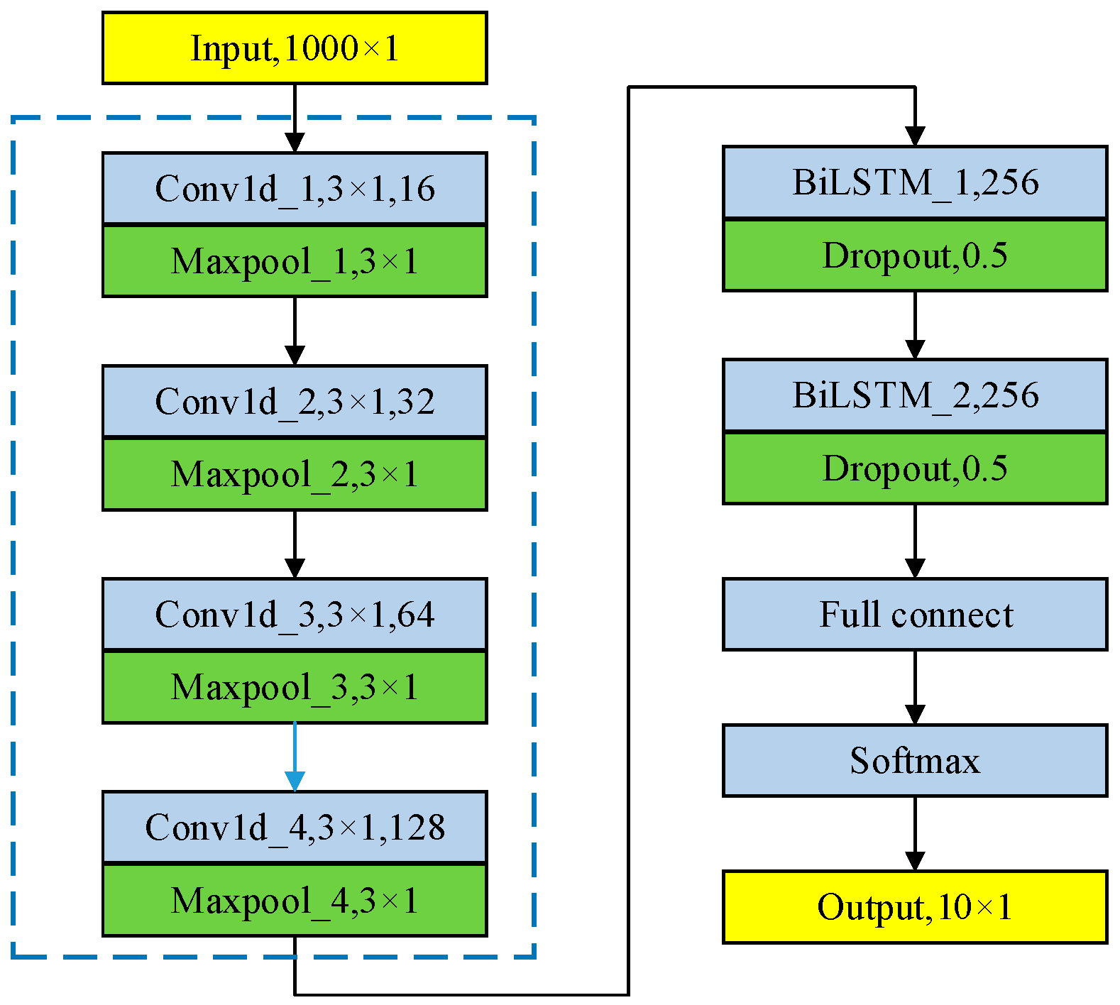
3.3. DCNN-BiLSTM Model

The 1DCNN layer can use less processing resources for feature extraction by arranging the identified features in a sparse matrix, which leads to better identification of correlations between features, reduces the number of parameters, and shortens the training time by a large amount of time. The BiLSTM layer is used to learn both forward and reverse time series data, and the hidden layer uses two units with the same inputs and connected to the same outputs, one processing the forward time series The hidden layer uses two units with the same input and connected to the same output, one processing the forward time series and the other processing the reverse time series. The combination of the two improves the training time while learning features better and achieving accurate recognition of large span time series data. In this paper, we combine the advantages of 1DCNN and BiLSTM to design a 1DCNN-BiLSTM-based fault diagnosis model, as shown in Figure 9.

The input signal to the signal input stage in the 1DCNN-BiLSTM model is a one-dimensional voltage signal of length 1000. According to the literature [22,24,25,26,27], combined with the requirements of circuit fault diagnosis scenarios of measurement and control systems, several experiments are conducted to set the model parameters. Firstly, the input signal is convolved, and the part of convolution is composed of four layers of convolutional layers and four layers of pooling layers, and the size of convolutional kernels are all 3, and the number of convolutional kernels in each layer is 16, 32, 64, and 128, respectively; and then two layers of BiLSTM layers are connected behind the convolutional network, and the hidden nodes are set to 256. Each BiLSTM layer is connected behind one Dropout layer, and the probability of the Dropout layer is set to 0.5; finally, the output of the BiLSTM network is connected to the fully connected layer, and the output of the simulated circuit fault category is output through the Softmax layer.

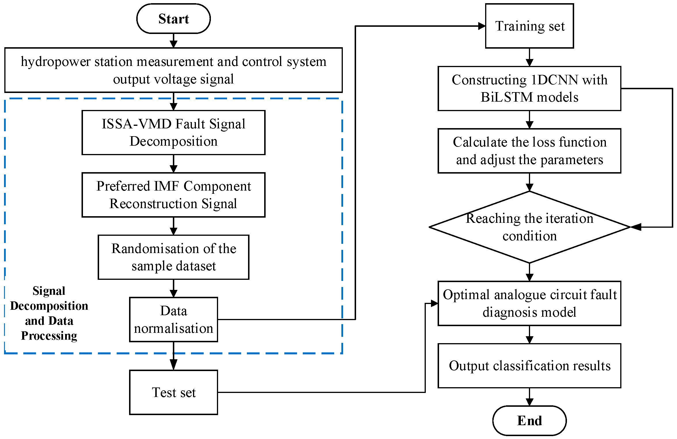
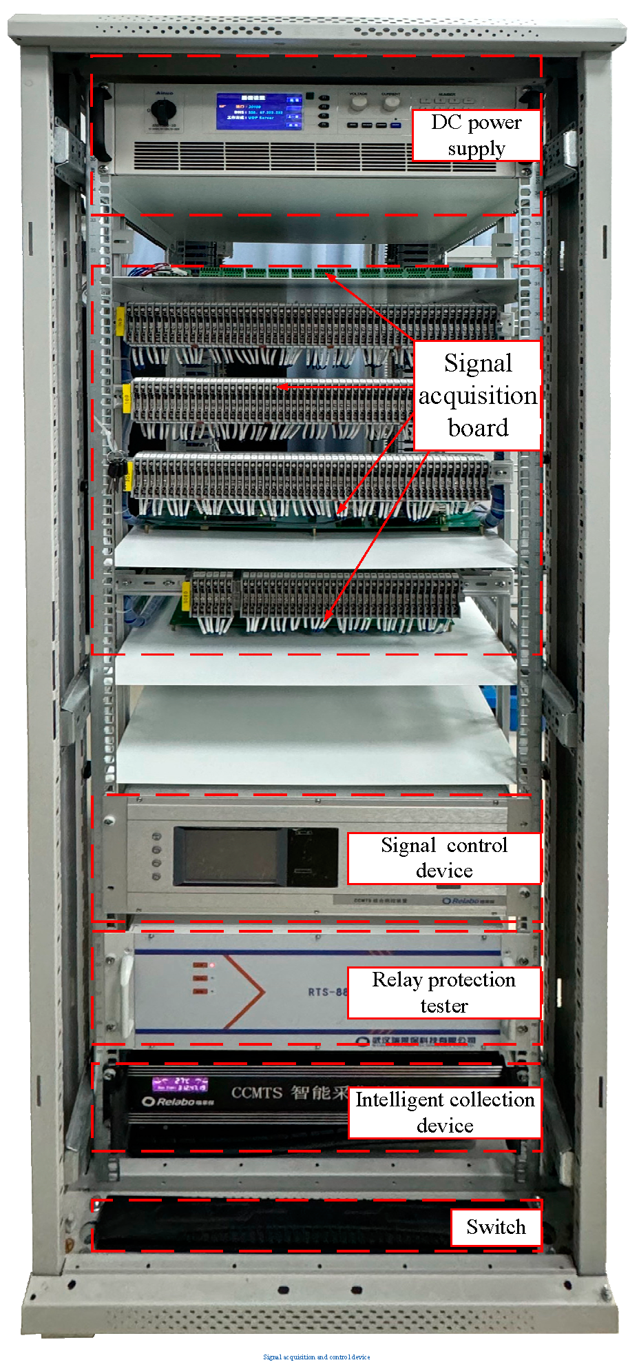
3.4. Troubleshooting Process for Hydropower Station Measurement and Control System

This paper proposes a fault diagnosis method for hydropower station measurement and control system based on the ISSA-VMD decomposition algorithm, which calculates the preferred IMF components for signal reconstruction and combines with 1DCNN-BiLSTM, which is mainly divided into four stages, namely, fault signal input, signal preprocessing, fault feature extraction, and fault diagnosis, and the fault diagnostic flowchart is shown in Figure 10, i.e., the fault diagnostic process is as follows:

(1)

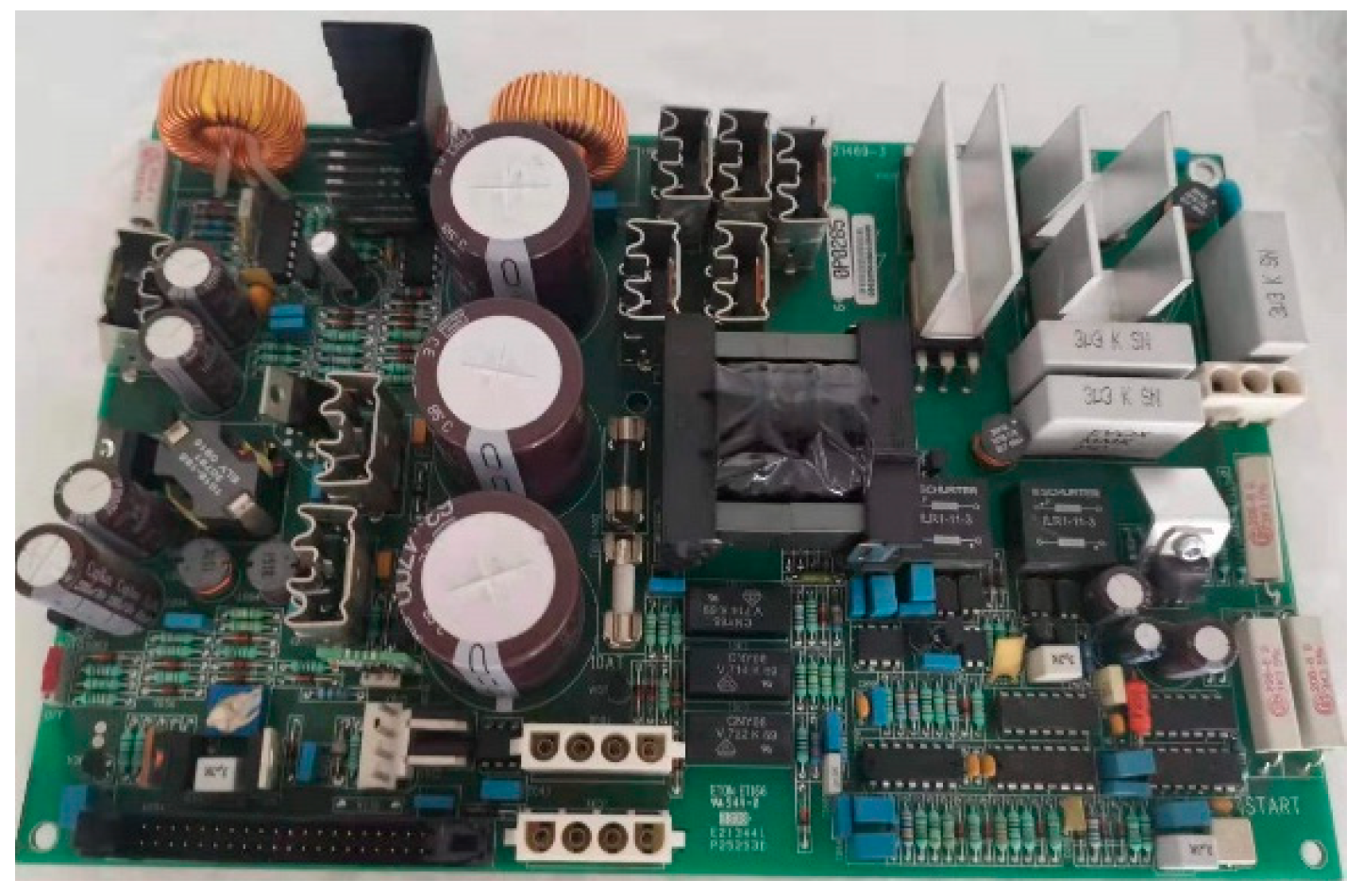
Signal acquisition: the output voltage signal of the measurement and control circuit of the hydropower station is taken as the signal input.

(2)

Signal decomposition: the ISSA-VMD algorithm is used to decompose the voltage signal output from the measurement and control circuit of the hydroelectric power station, and a number of IMF components are obtained.

(3)

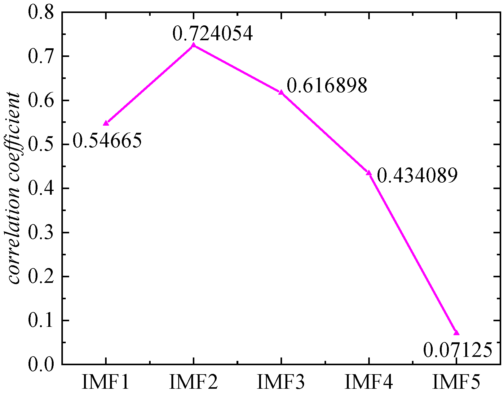
IMF component screening: by calculating the Pearson correlation coefficient of each IMF component, in order to screen out the effective IMF components.

(4)

Signal reconstruction: the new fault signal sequence is obtained by signal reconstruction of the screened IMF components to extract the effective feature information.

(5)

Fault feature extraction: the reconstructed fault signal is input into the 1DCNN-BiLSTM model to achieve deep self-extraction of fault features, and fault feature integration is performed at the fully connected layer.

(6)

Fault diagnosis: the extracted fault features are inputted into the softmax layer of the 1DCNN-BiLSTM model for fault classification, in order to realise the fault diagnosis of the hydropower station measurement and control system.

4. Experimental Validation

4.1. Simulation Analysis

A typical OPAMP high-pass filter circuit of hydropower station measurement and control system is selected to verify the effectiveness of the method. The literature [19] points out that analogue circuit combination faults have a greater impact on the output of the circuit compared to single faults, so for the test circuit, the data under single and combination faults are obtained by Pspice simulation software V16.6, respectively. Finally, a series of comparative experiments are conducted to evaluate the performance of the proposed parameter-optimized variational modal decomposition and 1DCNN-BiLSTM fault diagnosis method for hydropower station measurement and control system.

The four-OPAMP high-pass filter circuit is shown in Figure 11, and the Pspice sensitivity analysis is used to learn that R1, R3, R4, R9, C1 and C2 in the four-OPAMP high-pass filter circuit have a large impact on the output, so the fault states are simulated by setting the parameters of the four components, and the specific fault types are shown in

Table 4. Types of faults in four-OPAMP high-pass filter circuits.

Number	Fault Type	Nominal Value	Failure Value
F0	NF	/	/
F1	C1↑	5 nF	10 nF
F2	C1↓	5 nF	2.5 nF
F3	C2↑	5 nF	15 nF
F4	R4↓	6.2 kΩ	3 kΩ
F5	R3↑	6.2 kΩ	18 kΩ
F6	R1↑	6.2 kΩ	12 kΩ
F7	R9↓	1.6 kΩ	0.5 kΩ
F8	R1↑C1↓	6.2 kΩ, 5 nF	12 kΩ, 2.5 nF
F9	R3↓R9↑C2↓	6.2 kΩ, 1.6 kΩ, 5 nF	2 kΩ, 2.5 kΩ, 2.5 nF

. For each fault type, 1000 Monte Carlo analyses are performed respectively, generating a total of 1000 data samples, and the data set is divided into training set and test set in the form of 1:1.

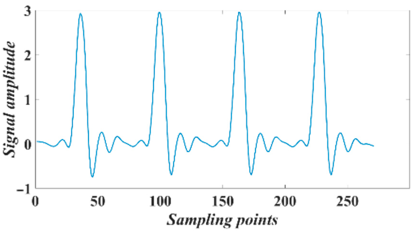
4.2. Fault Signal Decomposition and Analysis

To verify the advantages of ISSA, it is compared with SSA, GA and WOA. The values of the system parameters are set, i.e., τ = 0, init = 1, DC = 0, tol = 1 × 10⁻⁷, K ∈ [2, 7] and α ∈ [100, 2500], and the number of decision variables dim = 2. The maximum number of iterations for the four optimization algorithms, i.e., ISSA, SSA, GA, and WOA, itermax = 100, and the number of populations Num = 30, and all other parameters are set with reference to Table 2.

ISSA-VMD is used to decompose the signal, and its iterative convergence comparison results are shown in Figure 12.

From Figure 12, it can be seen that ISSA, SSA, WOA and GA reach convergence after the 9th, 11th, 15th and 13th iterations, at which time the fitness values are 3.454, 3.459, 3.465, 3.461, respectively. Compared with the other three algorithms, ISSA-VMD not only performs optimally in terms of the iterative convergence speed but also has the smallest fitness value, which indicates that it has faster optimization speed and stronger global search capability, and it shows that the introduction of Sine chaos mapping and adaptive t-distribution can effectively improve the SSA algorithm.

The ISSA-VMD decomposition is performed on the sample data with different fault types, and Figure 13 shows the original data waveforms under the F0–F9 fault state in the four-OPAMP high-pass filter circuit, which are decomposed by the ISSA-VMD algorithm, and the decomposition results are shown in Figure 14, and the optimal parameter combination of the VMD is obtained as [K,α] = [5300.42].

As can be seen in Figure 14, the frequency of each IMF component is concentrated in the center of its corresponding component, indicating that the IMF can successfully separate from the original fault signal and reduce the occurrence of modal aliasing. The original signal feature information contained in different IMF components is inconsistent, and the redundant information contained in the IMF components will affect the diagnosis results.

In order to filter out the effective IMF components, the Pearson correlation coefficient between the IMF components and the original signal is calculated, and then the original fault signal is reconstructed. The result of the correlation coefficient is shown in Figure 15.

From Figure 15, it is evident that the Pearson correlation coefficients for the IMF1-IMF3 components exceed the threshold value of 0.5. Consequently, these IMF components, characterized by correlation coefficients above 0.5, are filtered and utilized to reconstruct the fault signal waveforms. These reconstructed waveforms are subsequently fed into the fault classification model to generate the fault diagnosis results. The reconstructed signal waveforms are depicted in Figure 16.

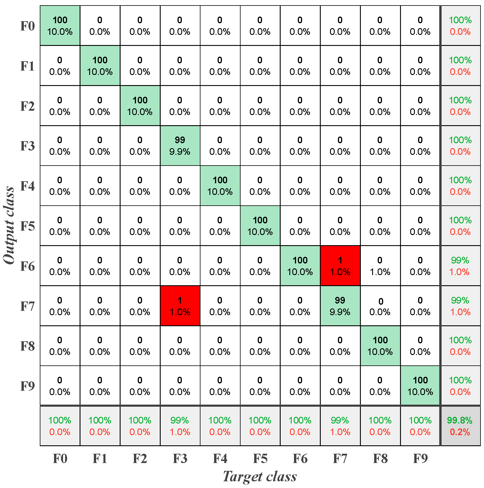
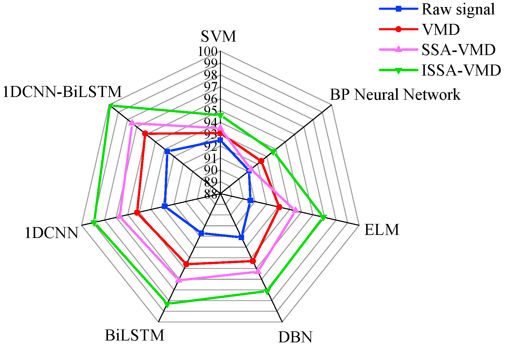
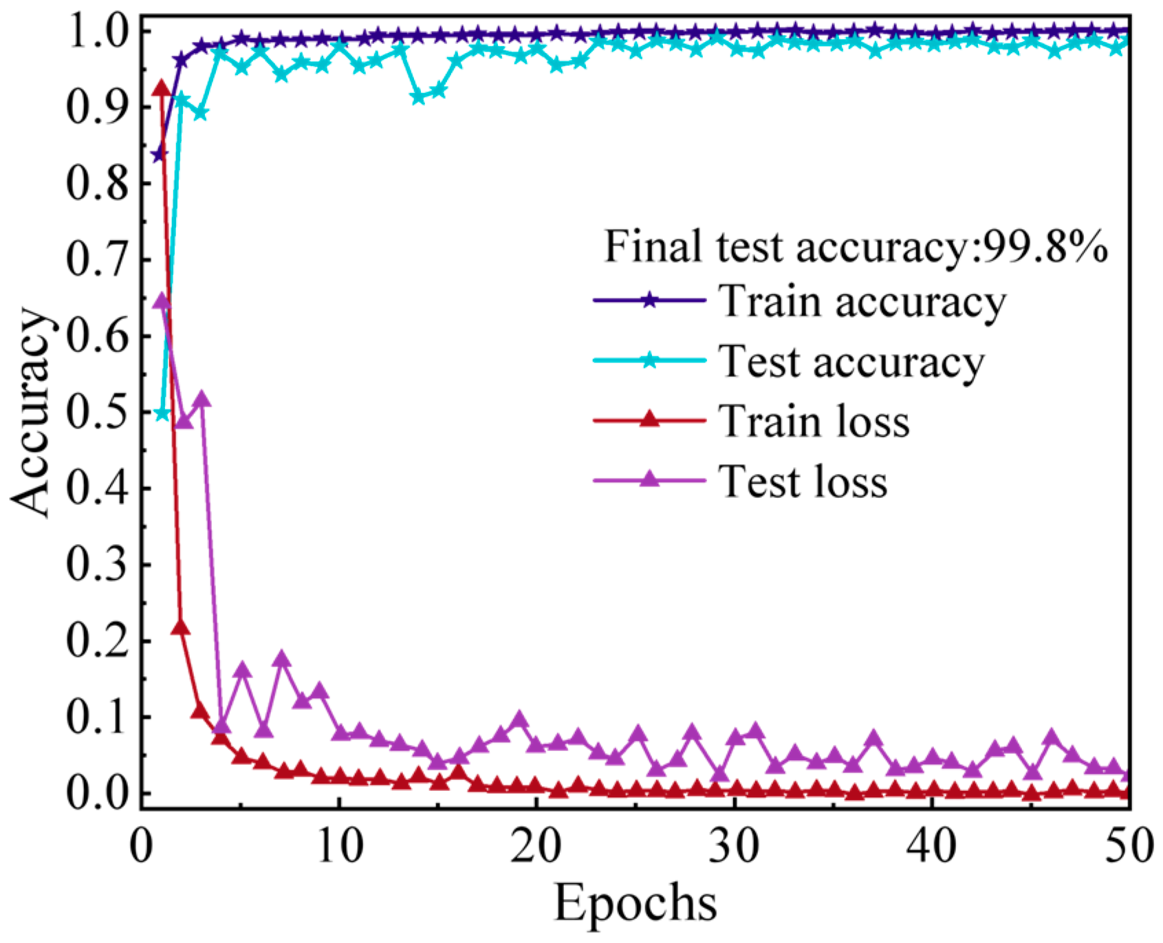
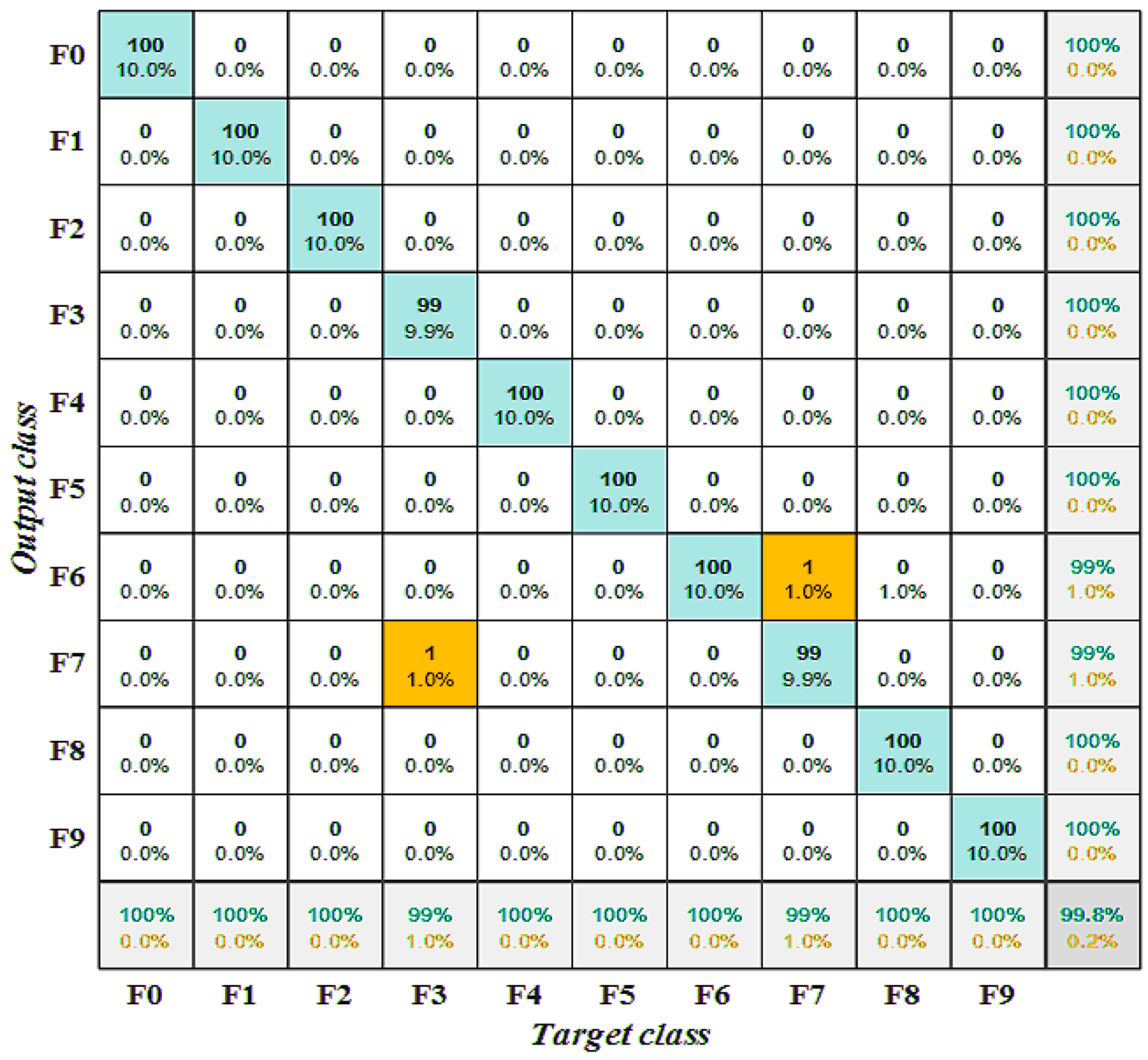
4.3. Fault Diagnosis Results and Analysis

In order to verify the reliability of the analogue circuit fault diagnosis model with parameter-optimized variational modal decomposition and 1DCNN-BiLSTM proposed in this paper, firstly, the Pearson’s correlation coefficient method is used to screen out the better IMF components of the fault signals that have been processed by the ISSA-VMD, and the preferred components are subjected to signal reconstruction in order to obtain a new signal sequence. Then, the reconstructed signal sequence is input to 1DCNN-BiLSTM, 1DCNN, BiLSTM, ELM, and BP neural networks, and SVM and DBN for fault diagnosis, respectively. Meanwhile, in order to verify the overall effectiveness and superiority of the ISSA-VMD algorithm proposed in this paper, the signal decomposition methods of SSA-VMD and VMD are selected for comparative analysis.

Under two different circuits, signal decomposition is performed separately using different signal decomposition methods and training set data with different fault types, and the reconstructed signal sequences under different fault states are input to seven classification models for model training. Finally, the test sets in two different circuits are input into the optimal fault diagnosis model for fault diagnosis validation.

Figure 17 shows the optimal model training curves for the parameter-optimized variational modal decomposition and 1DCNN-BiLSTM analogue circuit fault diagnosis method for the training set data of the four-OPAMP high-pass filtered circuits after 50 iterations, and the accuracy of the final test set reaches 99.8%. The confusion matrix of the analogue circuit fault diagnosis results of the method is shown in Figure 18.

As can be seen in Figure 18, there are only two misclassifications in the test set, misclassifying F7 fault type (R9↓) as F6 fault type (R1↑), and misclassifying F3 fault type (C2↑) as F7 fault type (R9↓), indicating that the method can be applied to fault diagnosis of analogue circuits.

In order to comprehensively compare the fault diagnosis effects of ISSA-VMD, SSA-VMD and VMD signal decomposition methods combined with 1DCNN-BiLSTM, 1DCNN, BiLSTM, ELM, and BP neural networks, and SVM, DBN classification methods, radar charts are chosen to visualize the accuracy of the different fault diagnosis models, and the comparison results are shown in Figure 19.

From the diagnostic results in Figure 19, it can be seen that the use of ISSA for parameter optimization of VMD combined with Pearson’s correlation coefficient for fault signal reconstruction not only improves the fault diagnosis accuracy of the analogue circuit but also adequately removes the ineffective fault feature information from the sample data. When the reconstructed signal sequence is applied to 1DCNN-BiLSTM, 1DCNN, BiLSTM, ELM, and BP neural networks and SVM and DBN fault classification models, the 1DCNN-BiLSTM model improves the fault diagnosis accuracy compared with other classification models. In summary, the diagnostic accuracy of all the analogue circuit fault diagnosis methods proposed in this paper is better than other methods.

4.4. Example Analyses

The above simulation circuit data were obtained by Pspice software, and in order to verify the effectiveness of its method in practical application, the power board card in the measurement and control circuit in a hydropower station was selected, and a fault classification experiment was carried out using the fault diagnosis experimental platform.

Figure 20 gives the fault diagnosis experimental platform, including a DC power supply, a four-layer signal acquisition board, a relay protection instrument, a control device, an intelligent acquisition device, and a switch. The board faults were simulated by replacing different components with different parameters, collecting fault sample data, and using signal decomposition and signal reconstruction methods to construct the fault data set.

The power supply board is shown in Figure 21, and the resistors and capacitors in its circuit have tolerances of 5% and 10%, respectively. When the actual value of the resistance or capacitance deviates by 50% relative to the standard value, the circuit fails, and the output voltage waveforms under the operating state of the circuit are obtained. Pspice sensitivity analysis was used to learn that the power board circuits R2, R5, C1 and C2 have a greater impact on the output, so by replacing four different components with different parameters, the fault states were simulated, the specific types of faults shown in

Table 5. Power board card circuit fault types.

Number	Fault Type	Nominal Value	Failure Value
F0	NF	/	/
F1	C1↑	5 nF	10 nF
F2	C1↓	5 nF	2.5 nF
F3	C2↓	5 nF	2.5 nF
F4	R2↑	3 kΩ	6 kΩ
F5	R2↓	3 kΩ	1.5 kΩ
F6	R5↑	2 kΩ	4 kΩ
F7	R2↑C1↓	3 kΩ, 5 nF	6 kΩ, 2.5 nF
F8	R2↓C1↑	3 kΩ, 5 nF	1.5 kΩ, 10 nF
F9	R2↓R5↑C2↓	3 kΩ, 2 kΩ, 5 nF	1.5 kΩ, 4 kΩ, 2.5 nF

. For each fault type, 20 samples were collected, resulting in a total of 200 data samples, as shown in Figure 22, and the data set was divided into training set and test set in the form of 1:1.

For the test data, according to the parameter settings in Section 4.2, four different methods were used to optimize VMD decomposition. The convergence curve comparison is shown in Figure 23, which is basically consistent with the simulation analysis results. ISSA-VMD performs the best.

Figure 24 shows the best model training curve after 50 iterations of the training set data for the power board card circuit, with 99.8% accuracy in the final test set. The confusion matrix of the fault diagnosis results of this method is shown in Figure 25. Comparing the fault diagnosis results of different signal decomposition methods in combination with different classification methods, a radar chart, shown in Figure 26, was used to visualize the accuracy of different fault diagnosis models.

As can be seen in Figure 24, there were only two misclassifications in the test set, misclassifying the F7 fault type (R9↓) as the F6 fault type (R1↑), and also misclassifying the F3 fault type (C2↑) as the F7 fault type (R9↓).

Based on the diagnostic results presented in Figure 26, the 1DCNN-BiLSTM model shows superior fault diagnosis accuracy compared to other classification models when applied to real-world circuit faults in the measurement and control systems of hydropower stations. To better illustrate the practical impact of these findings, we further analyzed the robustness and adaptability of the proposed method under various operational scenarios commonly encountered in hydropower stations, such as load fluctuations, environmental changes, and equipment aging.

The experimental results, derived from comprehensive measurement data, confirm the effectiveness of the proposed method. This high level of diagnostic accuracy suggests that the method is not only capable of identifying a wide range of fault types but is also resilient to different operating conditions. These results underline its practical value for enhancing fault diagnosis processes within hydropower measurement and control systems, thereby supporting more reliable and intelligent operational management in real-world applications.

5. Conclusions

To address the challenges in fault diagnosis for hydropower station measurement and control systems, this paper proposes a novel method combining ISSA-optimized VMD with a 1DCNN-BiLSTM model, which supports intelligent operation and maintenance of hydropower stations effectively.

• This study introduces Sine chaotic mapping and adaptive t-distribution to improve the uniformity of the sparrow population’s distribution within the search space, enhancing global search capabilities. These improvements resolve issues of premature convergence and local optima in traditional SSA, and their effectiveness is validated through comparative experiments.
• By using ISSA to optimize VMD parameters, the accuracy and efficiency of signal decomposition are significantly enhanced. Effective IMF components are selected based on the Pearson correlation coefficient, allowing for a reconstructed signal that reduces redundant information in the sample data and produces clearer, more informative sequences.
• A comprehensive comparison of various signal decomposition and fault classification methods demonstrates that the proposed method effectively diagnoses multiple fault types in hydropower station measurement and control system circuits. The experimental results indicate that this model significantly improves diagnostic accuracy, achieving an average recognition rate of 98.8% in both simulation and real-world analyses, underscoring its high applicability and value in practical hydropower fault diagnosis tasks.

References

1. Fan, J.; Yuan, W. Review of Parametric Fault Prediction Methods for Power Electronic Circuits. Eng. Res. Express 2021, 3, 042002. [Google Scholar] [CrossRef]
2. Jia, Z.; Liu, Z.; Gan, Y.; Vong, C.-M.; Pecht, M. A Deep Forest-Based Fault Diagnosis Scheme for Electronics-Rich Analog Circuit Systems. IEEE Trans. Ind. Electron. 2021, 68, 10087–10096. [Google Scholar] [CrossRef]
3. Zhang, C.; He, Y.; Yuan, L.; Xiang, S. Analog Circuit Incipient Fault Diagnosis Method Using DBN Based Features Extraction. IEEE Access 2018, 6, 23053–23064. [Google Scholar] [CrossRef]
4. Zhang, C.; Zha, D.; Wang, L.; Mu, N. A Novel Analog Circuit Soft Fault Diagnosis Method Based on Convolutional Neural Network and Backward Difference. Symmetry 2021, 13, 1096. [Google Scholar] [CrossRef]
5. Li, J.; Chen, W.; Han, K.; Wang, Q. Fault Diagnosis of Rolling Bearing Based on GA-VMD and Improved WOA-LSSVM. IEEE Access 2020, 8, 166753–166767. [Google Scholar] [CrossRef]
6. Khemani, V.; Azarian, M.H.; Pecht, M.G. Learnable Wavelet Scattering Networks: Applications to Fault Diagnosis of Analog Circuits and Rotating Machinery. Electronics 2022, 11, 451. [Google Scholar] [CrossRef]
7. Du, H.; Wang, J.; Qian, W.; Zhang, X. An Improved Sparrow Search Algorithm for the Optimization of Variational Modal Decomposition Parameters. Appl. Sci. 2024, 14, 2174. [Google Scholar] [CrossRef]
8. Lin, S.-L. Application Combining VMD and ResNet101 in Intelligent Diagnosis of Motor Faults. Sensors 2021, 21, 6065. [Google Scholar] [CrossRef]
9. Tang, S.; Yuan, S.; Zhu, Y. Data Preprocessing Techniques in Convolutional Neural Network Based on Fault Diagnosis Towards Rotating Machinery. IEEE Access 2020, 8, 149487–149496. [Google Scholar] [CrossRef]
10. Wang, Z.; Luo, Q.; Chen, H.; Zhao, J.; Yao, L.; Zhang, J.; Chu, F. A high-accuracy intelligent fault diagnosis method for aero-engine bearings with limited samples. Comput. Ind. 2024, 159, 104099. [Google Scholar] [CrossRef]
11. Sob, U.M.; Bester, H.L.; Smirnov, O.M.; Kenyon, J.S.; Grobler, T.L. Radio Interferometric Calibration Using a Complex Student’s t-Distribution and Wirtinger Derivatives. Mon. Not. R. Astron. Soc. 2020, 491, 1026–1042. [Google Scholar] [CrossRef]
12. Sharma, V.; Parey, A. Extraction of Weak Fault Transients Using Variational Mode Decomposition for Fault Diagnosis of Gearbox under Varying Speed. Eng. Fail. Anal. 2020, 107, 104204. [Google Scholar] [CrossRef]
13. He, Z.; Chen, G.; Hao, T.; Teng, C.; Hou, M.; Cheng, Z. Weak Fault Detection Method of Rolling Bearing Based on Testing Signal Far Away from Fault Source. J. Mech. Sci. Technol. 2020, 34, 1035–1048. [Google Scholar] [CrossRef]
14. Li, Y.; Huang, D.; Qin, Z. A Classification Algorithm of Fault Modes-Integrated LSSVM and PSO with Parameters’ Optimization of VMD. Math. Probl. Eng. 2021, 2021, 6627367. [Google Scholar] [CrossRef]
15. Xu, Z.; Mei, X.; Wang, X.; Yue, M.; Jin, J.; Yang, Y.; Li, C. Fault Diagnosis of Wind Turbine Bearing Using a Multi-Scale Convolutional Neural Network with Bidirectional Long Short Term Memory and Weighted Majority Voting for Multi-Sensors. Renew. Energy 2022, 182, 615–626. [Google Scholar] [CrossRef]
16. Yan, X.; Jia, M.; Xiang, L. Compound Fault Diagnosis of Rotating Machinery Based on OVMD and a 1.5-Dimension Envelope Spectrum. Meas. Sci. Technol. 2016, 27, 075002. [Google Scholar] [CrossRef]
17. Zhou, F.; Yang, X.; Shen, J.; Liu, W. Fault Diagnosis of Hydraulic Pumps Using PSO-VMD and Refined Composite Multiscale Fluctuation Dispersion Entropy. Shock Vib. 2020, 2020, 8840676. [Google Scholar] [CrossRef]
18. Yang, K.; Wang, G.; Dong, Y.; Zhang, Q.; Sang, L. Early Chatter Identification Based on an Optimized Variational Mode Decomposition. Mech. Syst. Signal Proc. 2019, 115, 238–254. [Google Scholar] [CrossRef]
19. Wu, Q.; Lin, H. Short-Term Wind Speed Forecasting Based on Hybrid Variational Mode Decomposition and Least Squares Support Vector Machine Optimized by Bat Algorithm Model. Sustainability 2019, 11, 652. [Google Scholar] [CrossRef]
20. Xue, J.; Shen, B. A Novel Swarm Intelligence Optimization Approach: Sparrow Search Algorithm. Syst. Sci. Control Eng. 2020, 8, 22–34. [Google Scholar] [CrossRef]
21. Wen, L.; Li, X.; Gao, L. A New Two-Level Hierarchical Diagnosis Network Based on Convolutional Neural Network. IEEE Trans. Instrum. Meas. 2020, 69, 330–338. [Google Scholar] [CrossRef]
22. Chen, L.; Khan, U.S.; Khattak, M.K.; Wen, S.; Wang, H.; Hu, H. An Effective Approach Based on Nonlinear Spectrum and Improved Convolution Neural Network for Analog Circuit Fault Diagnosis. Rev. Sci. Instrum. 2023, 94, 054709. [Google Scholar] [CrossRef] [PubMed]
23. Zhang, K.; Su, J.; Sun, S.; Liu, Z.; Wang, J.; Du, M.; Liu, Z.; Zhang, Q. Compressor Fault Diagnosis System Based on PCA-PSO-LSSVM Algorithm. Sci. Prog. 2021, 104, 00368504211026110. [Google Scholar] [CrossRef] [PubMed]
24. Jiang, Y.; Xia, L.; Zhang, J. A Fault Feature Extraction Method for DC-DC Converters Based on Automatic Hyperparameter-Optimized 1-D Convolution and Long Short-Term Memory Neural Networks. IEEE J. Emerg. Sel. Top. Power Electron. 2022, 10, 4703–4714. [Google Scholar] [CrossRef]
25. Rossi, A.; Hagenbuchner, M.; Scarselli, F.; Tsoi, A.C. A Study on the Effects of Recursive Convolutional Layers in Convolutional Neural Networks. Neurocomputing 2021, 460, 59–70. [Google Scholar] [CrossRef]
26. Dragomiretskiy, K.; Zosso, D. Variational Mode Decomposition. IEEE Trans. Signal Process. 2014, 62, 531–544. [Google Scholar] [CrossRef]
27. Wang, J.; Guo, J.; Wang, L.; Yang, Y.; Wang, Z.; Wang, R. A Hybrid Intelligent Rolling Bearing Fault Diagnosis Method Combining WKN-BiLSTM and Attention Mechanism. Meas. Sci. Technol. 2023, 34, 085106. [Google Scholar] [CrossRef]
28. Wang, L.; Zhou, D.; Zhang, H.; Zhang, W.; Chen, J. Application of Relative Entropy and Gradient Boosting Decision Tree to Fault Prognosis in Electronic Circuits. Symmetry 2018, 10, 495. [Google Scholar] [CrossRef]
29. Lundgren, A.; Jung, D. Data-Driven Fault Diagnosis Analysis and Open-Set Classification of Time-Series Data. Control Eng. Pract. 2022, 121, 105006. [Google Scholar] [CrossRef]
30. Wang, R.; Zhan, Y.; Chen, M.; Zhou, H. Fault Diagnosis Technology Based on Wigner-Ville Distribution in Power Electronics Circuit. Int. J. Electron. 2011, 98, 1247–1257. [Google Scholar] [CrossRef]
31. Ma, Z.; Zhang, X.; Yuan, H.; Zhu, X.; Yang, F.; Zhang, E.; Zhang, Q.; Yao, Y. An Adaptive T-Distribution Variation Based HS Algorithm for Power System ED. In Recent Developments in Intelligent Computing, Communication and Devices; Wu, C.H., Patnaik, S., Popentiu Vlãdicescu, F., Nakamatsu, K., Eds.; Springer: Singapore, 2021; pp. 125–133. [Google Scholar] [CrossRef]
Figure 1. Flowchart of ISSA algorithm.
Energies 17 05686 g001
Figure 2. Benchmarking function f1 image and optimization algorithm’s optimization process. (a) Benchmarking functions f1. (b) Optimization and convergence process.
Energies 17 05686 g002
Figure 3. Benchmarking function f2 image and optimization algorithm’s optimization process. (a) Benchmarking functions f2. (b) Optimization and convergence process.
Energies 17 05686 g003
Figure 4. Benchmarking function f3 image and optimization algorithm’s optimization process. (a) Benchmarking functions f3. (b) Optimization and convergence process.
Energies 17 05686 g004
Figure 5. Benchmarking function f4 image and optimization algorithm’s optimization process. (a) Benchmarking functions f4. (b) Optimization and convergence process.
Energies 17 05686 g005
Figure 6. Benchmarking function f5 image and optimization algorithm’s optimization process. (a) Benchmarking functions f5. (b) Optimization and convergence process.
Energies 17 05686 g006
Figure 7. Benchmarking function f6 image and optimization algorithm’s optimization process. (a) Benchmarking functions f6. (b) Optimization and convergence process.
Energies 17 05686 g007
Figure 8. Flowchart of ISSA optimization of VMD parameters.
Energies 17 05686 g008
Figure 9. 1DCNN-BiLSTM model.
Energies 17 05686 g009
Figure 10. Analogue circuit fault diagnosis flow.
Energies 17 05686 g010
Figure 11. Quad OPAMP high pass filter circuit.
Energies 17 05686 g011
Figure 12. Comparison of iterative convergence of the four methods.
Energies 17 05686 g012
Figure 13. Waveforms in F0-F9 fault condition.
Energies 17 05686 g013
Figure 14. ISSA-VMD signal decomposition results for F7.
Energies 17 05686 g014
Figure 15. IMF Component Correlation Coefficient Values.
Energies 17 05686 g015
Figure 16. Reconstructed signal waveform.
Energies 17 05686 g016
Figure 17. Training curves for the four-OPAMP high-pass filter circuit model.
Energies 17 05686 g017
Figure 18. Confusion matrix for four-OPAMP high-pass filtering circuits.
Energies 17 05686 g018
Figure 19. Results of different fault diagnosis models for four OPAMP high pass filter circuits.
Energies 17 05686 g019
Figure 20. Fault diagnosis experiment platform of hydropower station measurement and control system.
Energies 17 05686 g020
Figure 21. Power supply board of hydropower station measurement and control system.
Energies 17 05686 g021
Figure 22. Platform measured output voltage waveform.
Energies 17 05686 g022
Figure 23. Comparison of iterative convergence of the four methods.
Energies 17 05686 g023
Figure 24. Model training curves for the power board card circuits.
Energies 17 05686 g024
Figure 25. Confusion Matrix for Power Board Circuitry.
Energies 17 05686 g025
Figure 26. Results of different troubleshooting models for power board card circuits.
Energies 17 05686 g026