Article

Low-Carbon Dispatch Method for Active Distribution Network Based on Carbon Emission Flow Theory

1
Electric Power Science Research Institute, State Grid Tianjin Electric Power Company, Tianjin 300384, China
2
State Grid Tianjin Electric Power Company, Tianjin 300010, China
3
School of Electrical and Information Engineering, Tianjin University, Tianjin 300072, China
*
Author to whom correspondence should be addressed.
Energies 2024, 17(22), 5610; https://doi.org/10.3390/en17225610
Submission received: 5 September 2024 / Revised: 28 September 2024 / Accepted: 1 October 2024 / Published: 9 November 2024
(This article belongs to the Section B: Energy and Environment)

Abstract

:
In the context of integrating renewable energy sources such as wind and solar energy sources into distribution networks, this paper proposes a proactive low-carbon dispatch model for active distribution networks based on carbon flow calculation theory. This model aims to achieve accurate carbon measurement across all operational aspects of distribution networks, reduce their carbon emissions through controlling unit operations, and ensure stable and safe operation. First, we propose a method for measuring carbon emission intensity on the source and network sides of active distribution networks with network losses, allowing for the calculation of total carbon emissions throughout the operation of networks and their equipment. Next, based on the carbon flow distribution of distribution networks, we construct a low-carbon dispatch model and formulate its optimization problem within a Markov Decision Process framework. We improve the Soft Actor–Critic (SAC) algorithm by adopting a Gaussian-distribution-based reward function to train and deploy agents for optimal low-carbon dispatch. Finally, the effectiveness of the proposed model and the superiority of the improved algorithm are demonstrated using a modified IEEE 33-bus distribution network test case.

1. Introduction

With the rapid growth of the global economy and population, energy demand is rising, and the impact of carbon emissions on the environment is becoming increasingly significant. To address environmental challenges, some regions, including the United States [1], Europe [2], and China [3], have introduced relevant policies and plans to reduce carbon emissions. The global power industry is accelerating its transition towards low-carbon development, with sustainable energy gradually replacing traditional energy sources and becoming a crucial component of energy structure adjustment. An important direction in the current development of decarbonization in the power industry is the utilization of active distribution networks (ADNs) as the primary carrier for distributed energy resources, such as wind and photovoltaic energy. These networks facilitate the development and utilization of renewable energy sources, reduce the consumption of fossil fuels, and contribute to achieving cleaner and lower carbon emissions [4,5].
The problem of low-carbon dispatch in ADNs begins with an accurate representation of carbon emissions from their operational processes. The use of equivalent transformations is currently more frequently studied in power system control problems. Xu et al. [6] used new energy in a distribution network as its carbon emission reduction indicator. Chen et al. [7] fit the carbon emissions of a unit and used conversion coefficients to convert the carbon emissions into economic costs. In order to describe the economic cost of carbon emissions in more detail, Qing et al. [8] took into account carbon emission taxes, carbon trading, and the penalty cost of wind and solar power abandonment. Chen et al. [9] took the economic benefits brought by the purchase and sale of carbon emission allowances as the objective function in the context of carbon trading. However, the results of such equivalent conversion methods are largely affected by the reasonableness of the conversion coefficients and the reasonableness of the economic model, ignoring the impact of time and space changes on the carbon emissions of distributed equipment. Since electricity production is driven by electricity consumption, some studies have shown that the demand side can be considered as the main cause of carbon emissions [10]. A number of countries have introduced carbon market or carbon tax policies that specify that in addition to power producers being responsible for carbon emissions, electricity consumers are also responsible for carbon emissions. Under these policies, electricity consumers are supposed to pay for the carbon emissions generated from the production of the electricity they consume, which can be calculated by multiplying the electricity consumption by the grid carbon emission factor. Therefore, the policy requires more timely and spatially differentiated carbon emission intensities to calculate and charge consumers according to their true level of carbon emission responsibility. Carbon emission flow evaluation results can provide consumers with timely and regionally differentiated carbon emission signals to inform the implementation and settlement of consumer-side charges. In addition, with appropriate incentive programs, this carbon emission distribution information can guide active carbon emission reduction on the demand side, further promoting low-carbon operation and planning of the power system. By employing the concept of carbon emission flow (CEF) as a virtual network flow, Kang et al. [11,12] networked CEF, attached carbon emission flow to the active current of the power system, analyzed and calculated the carbon emission generated in each link of energy production, transmission, and consumption, and tracked the carbon distribution in a power network. However, this model does not consider the power losses in lines in order to simplify calculations, while the line loss rate in ADNs is usually higher than that of the main network, so the line losses are not negligible, and a CEF model for ADNs is needed.
The large number of sustainable energy sources, such as wind power and photovoltaic sources, connected to the grid has transformed the traditional distribution network into an active network that actively controls the bidirectional flow of power, i.e., an ADN. At the same time, the distributed sustainable energy output is characterized by randomness, volatility, and intermittency [13], and its high penetration rate affects the power balance, power quality, and power supply reliability of the distribution network [14]. Distributed energy storage systems are crucial for addressing the challenges of intermittent new energy output and the poor temporal and spatial matching of distribution network loads. Implementing reasonable and effective energy storage control strategies can lead to the efficient operation of distribution networks [15]. In order to characterize sustainable energy uncertainty, the study [16] has established predictive probabilistic models for wind power and photovoltaic power and established an optimal dispatch method based on uncertainty boundaries; the study [17] also predicts new energy outputs and loads on dispatch days by using historical and weather data, but both probabilistic models and model-free prediction methods inevitably lead to the accumulation of errors and are only applicable to some specific scenarios. Compared with the stochastic sequential decision-making problem with continuous decision variables for optimal dispatch of distribution networks taking into account the uncertainty of new sustainable energy [18], deep reinforcement learning, as a model-free method, does not need to predict uncertainty in advance and, at the same time, is able to deal with higher-dimensional and complex state spaces [19]. Cao et al. [20] used a proximal policy optimization algorithm to solve a Markov decision problem for the dispatch of renewable energy and energy storage devices in distribution networks to assess the economics of distribution network operations. Hosseini et al. [21] optimized the reinforcement learning exploration process and imposed penalties on infeasible solutions to ensure the feasibility and optimality of training results. Xing et al. [22] used a graph reinforcement learning approach to solve the real-time optimal dispatch problem for an active distribution network, combining the topological characteristics of the distribution network and using a graph attention mechanism to extract and aggregate the node and line information in each training round to improve the data fusion capability of intelligent systems. Lu et al. [23] used the dual-DQN algorithm to construct a multiple-intelligent-body system, with the goal of minimum network loss and voltage deviation, and the two intelligent systems provide each other with incentives and strategies to achieve optimal problem-solving strategies. However, the aforementioned studies have focused on the economic and security aspects of distribution network operations. There is a noticeable gap in research concerning methods to address the low-carbon operation challenges of distribution networks.
In summary, this paper proposes a low-carbon dispatch method for ADNs, optimizes the CEF theory according to the nature of ADNs, proposes a carbon emission flow calculation method considering the network loss, and establishes a control framework for gas units and energy storage devices with low-carbon dispatch for ADNs on this basis, and under a series of constraints to ensure the safe and stable operation of ADNs, trains and applies deep reinforcement learning intelligence to achieve the lowest carbon emission control. The main innovations and contributions of this paper are as follows:
(1)
Based on the CEF theory, the dynamic carbon emission intensity calculation model of gas units, energy storage equipment, and a lossy ADN is established to realize the carbon emission measurement of each link. On this basis, a low-carbon dispatch model is proposed for distributed sustainable energy access scenarios, taking into account operational safety and low-carbon benefits.
(2)
The ADN low-carbon dispatch problem is modeled as a Markov decision-making process, which takes into account the uncertainties caused by carbon emission intensity changes in the main network, load changes, and changes in distributed sustainable energy generation, and improves the SAC algorithm of deep reinforcement learning by adopting a Gaussian distribution reward function sampling strategy, which effectively improves the stability of the training process of the intelligence and the algorithm performance.

2. Distributed Power Modeling for ADNs

In ADNs, distributed power sources mainly include gas-fired units, energy storage devices, and sustainable energy sources such as photovoltaic power generation and wind power generation, which are coordinated with the main grid power supply dispatch to jointly meet the power demand. The structure of the carbon emission flow model of an ADN is shown in Figure 1. In the study of this paper, the equipment that performs power dispatch is gas-fired units and energy storage equipment, and their operational mathematical models and carbon emission characteristics are explained in this section.

2.1. Gas Unit Model

The gas unit converts thermal energy produced by gas combustion into mechanical energy and then converts the mechanical energy into electrical energy through a generator, which has high flexibility and fast start-up capability and can respond quickly to changes in power demand [24]. The operation of the gas-fired unit is limited by the output power and climbing power, and its operation is mathematically modeled as follows:
p MT ( t ) p MT max
p MT down p MT ( t ) p MT ( t 1 ) p MT up
where pMT(t) is the output power of the gas unit at the time t; Hg indicates the calorific value of natural gas; ξg indicates the gas unit gas-to-electricity conversion efficiency; Mg(t) indicates the amount of natural gas used; p MT max is the maximum value of the output power of the gas unit; p MT down and p MT up are the minimum and maximum value of the climbing power of the gas unit, respectively.
We define the carbon intensity of a generating unit as the amount of carbon dioxide emitted per kWh of electricity produced, in gCO2/kWh. The magnitude of the carbon intensity of a gas-fired generating unit is largely dependent on the efficiency of the equipment and the composition of the natural gas, usually ranging from 350 gCO2/kWh to 600 gCO2/kWh.

2.2. Energy Storage Equipment Model

The electric energy storage devices in ADNs realize the regulation effect by charging and discharging at different moments, and the process of charging and discharging will also have an impact on the carbon emission of the distribution system.
Charge state is an important operation index for electric energy storage, defined as the ratio of the remaining capacity of the battery to the nominal capacity, and deep charging and discharging will cause damage to the energy storage equipment [25]. Therefore, in order to ensure the healthy operation of electric energy storage equipment, it is necessary to limit its charging and discharging power and charge state. Assuming that the charging and discharging power of the electric energy storage device is the same, its operation mathematical model is as follows:
S O C ( t ) = S O C ( t 1 ) p ESS ( t ) η ESS Δ t E capacity , p ESS ( t ) 0 S O C ( t 1 ) p ESS ( t ) Δ t E capacity η ESS , p ESS ( t ) > 0
S O C ESS min S O C ( t ) S O C ESS max
p ESS min p ESS ( t ) p ESS max
where pESS(t) indicates the charging and discharging power at the time t, for which a negative value indicates the charging state of the equipment and a positive value indicates the discharging state; p ESS min and p ESS max are the lower limit and upper limit; η ESS  is the charging and discharging efficiency of the energy storage equipment; SOC(t) indicates the charging state of the energy storage equipment at the time; S O C ESS min and S O C ESS max are the lower limit and upper limit.
Energy storage devices produce very little carbon emissions of their own during operation, which is negligible, but the transfer of carbon emissions from their storage of released electricity needs to be analyzed. Considering the different levels of carbon emissions generated per unit of electricity produced as an attribute, the energy storage device is equivalent to an electrical load when it is in the charging state, which cumulatively stores a mixture of electricity with different levels of carbon emissions. We define QESS(t1) as the amount of electricity stored by the storage device from the beginning t0 to the end of the charging cycle t1; FESS(t1) represents the amount of QESS(t1) carbon emissions generated during production:
Q ESS ( t 1 ) = S O C ( t 0 ) E C + t 0 t 1 p ESS ( t ) d t
F ESS ( t 1 ) = F ESS ( t 0 ) + t 0 t 1 e n i ( t ) p ESS ( t ) d t
where eni(t) denotes the carbon emission factor of the grid side of the access point i of the energy storage device at the time t, and pESS(t) is the charging power.
Combined with the carbon emission of a single cycle of energy storage equipment and the carbon emission transfer analysis of charging and discharging quantity, the carbon emission factor model of energy storage equipment operation is established: the carbon emission factor of discharging is constant from the state of charging to the state of discharging until the end of discharging into the next charging and discharging cycle of the energy storage equipment:
e ESS = F ESS ( t 1 ) + F cycle Q ESS ( t 1 ) η ESS
where η ESS is the conversion efficiency of charging and discharging of the energy storage device.

3. Carbon Emission Flow Theory for ADNs

Carbon emissions from the power system come from the power production at the source side, but in the final analysis, the load side of the distribution network is the source that guides the power production at the source side. Based on the CEF theory, this section proposes a carbon flow calculation model for ADNs taking line loss into account and establishes a source–network correlation analysis.

3.1. Calculation of Carbon Emission Distribution in ADNs

The CEF theory focuses on the analysis of the production, transfer, and consumption of carbon costs in the power system and combines the carbon emission flow with the power flow to quantitatively represent the carbon emissions contained in the power flowing through a particular branch to obtain the carbon emission distribution in the power system network [26].
We define the carbon flow rate R as the carbon emission per unit time in tCO2/h. We define the branch carbon flow density ρs for a branch s as the ratio of the carbon flow rate Rs to the active power flow Ps.
ρ s = R s P s
The carbon potential describes the relationship between the carbon flow rate of a node and the active power flow, and in combination with Equation (10), the carbon potential enj of node j is calculated as shown in the following equation:
e n j = s L j + P s ρ s s L j + P s = s L j + R s s L j + P s
where L j + is the set of branches of the power flow into the node.
The ADN’s voltage levels are low, and the total share of electric energy lost in the lines is large and often non-negligible [27]. The above carbon potential calculation method does not consider the power loss in the lines. Therefore, we add virtual loss nodes in the middle of each branch for the ADN to transform the lossy network into a lossless network.
Figure 2 demonstrates the process of line lossless processing; nodes No. 1 and No. 2 are the original nodes of the distribution network, and node No. 3 is the virtual node of the new loss of line j. The calculation of carbon potential evnj at the virtual node is the same as that at the real node, as shown in Equation (11).
e v n j = s L t + P s ρ s s L t + P s = e n i
For a node connected to a unit, its nodal carbon potential enj in the case of active unit injection is determined by the combination of the CEF generated by the generating unit connected to the node and the CEF into the node from other nodes:
e n j = s L j + P s ρ s + g G j + P g e g s L j + P s + g G j + P g
where Ps is the branch active power flow of branch s after equating to a lossless network, G j + is the set of injected units at node j, and Pg and eg denote the injected power of the units at node j and the carbon intensity of the units, respectively.

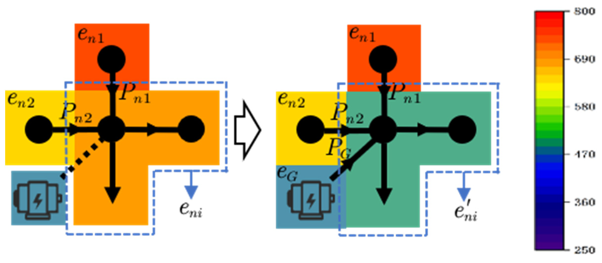
3.2. Dynamic Effects of Distributed Power Sources on Nodal Carbon Potentials

According to the definition of node carbon potential, in the case that a node j in the ADN is not connected to a distributed power source, the node carbon potential is only related to the node carbon potential flowing into that node with the power flow. And the inflow power to this node in the distribution network is equal to the total amount of its nodal load and sub-nodal load P0. According to Equation (12), the current nodal carbon potential is obtained as
e n j = s L j + , i Ω j + P s e n i P 0
where Ω j + is the set of injected power nodes at node j. When the generating equipment with carbon emission factor eg is connected to the node, its generating power Pg replaces a certain input power flow, and the carbon potential of node j becomes
e n j = ( P 0 P G ) e n j + P g e g P 0
The carbon potential change before and after the node is derived from Equations (13) and (14) as shown in Equation (15).
Δ e n j = e n j e n j = P g ( e g e n j ) P 0
As shown in Figure 3, when the outflow of node i connected to the generating equipment is fixed, the larger the difference between the original node carbon potential and the carbon emission factor of the generating equipment, or the larger the injected power of the generating unit, the larger the change in the node carbon potential before and after. Therefore, the operation status can be judged according to the carbon potential difference of the nodes: when the node carbon potential is higher than the carbon emission factor of the generating unit, the carbon emission intensity at the node load is reduced by increasing the input power of the generating unit.

4. Low-Carbon Dispatch Model for ADN

In this section, the objective function and model constraints for the low-carbon dispatch of ADNs are proposed based on CEF theory to construct a complete low-carbon optimal dispatch model for ADNs.

4.1. The Objective Function

Let there be a total of K distributed generating units in the distribution network, containing KW wind turbines, KP photovoltaic power plants, KM gas turbines, and another M energy storage devices. Minimizing the total carbon emissions generated from the operation of the main grid and the distribution grid during the dispatch cycle T is taken as the objective function:
m i n E T = t = 0 T P Grid ( t ) e Grid ( t ) + i = 1 K p G i ( t ) e G i + p ESS j ( t ) e ESS j ( t ) Δ t
where ET denotes the total carbon emissions during the dispatch cycle; PGrid(t) and eGrid(t) denote the active power and carbon potential of the main network at moment t; PGi(t) denotes the active output at moment t, and eGi(t) denotes carbon potential of the i-th distributed generator; PESSj(t) is the power of the j-th storage device, and eESSj(t) is the carbon potential, which is computed from Equation (8); and Δt is the data sampling interval
In the dispatch model, the power demand of the distribution network loads needs to be satisfied, so the power PGrid(t) input from the main network to the distribution network is calculated from the power balance constraints:
P Grid ( t ) = P Load ( t ) + P ESS ( t ) P MT ( t ) + P PV ( t ) + P WT ( t )
where PMT(t), PPV(t), and PWT(t) are the total output power of gas turbine, photovoltaic, and wind turbine at time t; PESS(t) is the total power of energy storage equipment; PLoad(t) is the total load of distribution network.

4.2. The Constraints

To ensure the stable and normal operation of the ADN, the constraints of the dispatch model include the distribution network current constraints, security constraints, stable operation constraints, and the operation constraints of each device.
(1)
Power flow constraints
P i ( t ) = U i ( t ) j = 1 N U j t B i , j ( t ) sin θ i , j ( t ) + G i , j ( t ) cos θ i , j ( t ) Q i ( t ) = U i ( t ) j = 1 N U j t G i , j ( t ) sin θ i , j ( t ) B i , j ( t ) cos θ i , j ( t )
where Pi(t) and Qi(t) denote the active and reactive power of node i at time t, respectively; Ui(t) and Uj(t) represent the voltage values of node i and node j at time t, respectively; Gi,j(t) and Bi,j(t) denote the conductance and conductance of node i and j, respectively; and θi,j(t) denotes the phase angle difference of node i and j.
(2)
Security constraints
U i min U i ( t ) U i max
I i , j 2 ( t ) I i , j 2 max
P i , j ( t ) P i , j max
Q i , j ( t ) Q i , j max
where U i max and U i min are the node voltage upper and voltage lower limits; I i , j 2 (t) is the line i-j current squared; I i , j 2   max (t) is the thermal capacity limit of the line; Pi,j(t) and Qi,j(t) denote the active and reactive power of line i-j; P i , j max and Q i , j max denote the maximum power limit of the line.
(3)
Stabilization constraints
Nodal voltage deviation is an important indicator of power quality in distribution networks [28]. We define the maximum deviation voltage ratio Δ U max ( t )  in distribution networks as
Δ U max ( t ) = max i N | U i ( t ) U i , ref | U i , ref
where Ui(t) denotes the voltage value of node i at time t; Ui,ref is the reference voltage value of node i. In order to ensure the voltage stability of the distribution network, the voltage deviation needs to be constrained within the ideal range:
Δ U max ( t ) Δ U max
(4)
Unit operating constraints
The operation of gas-fired generating units and energy storage devices satisfies the operational constraints of Equations (1)–(5) in Section 1.

5. Solving Low-Carbon Dispatch Model for ADN Based on Improved SAC

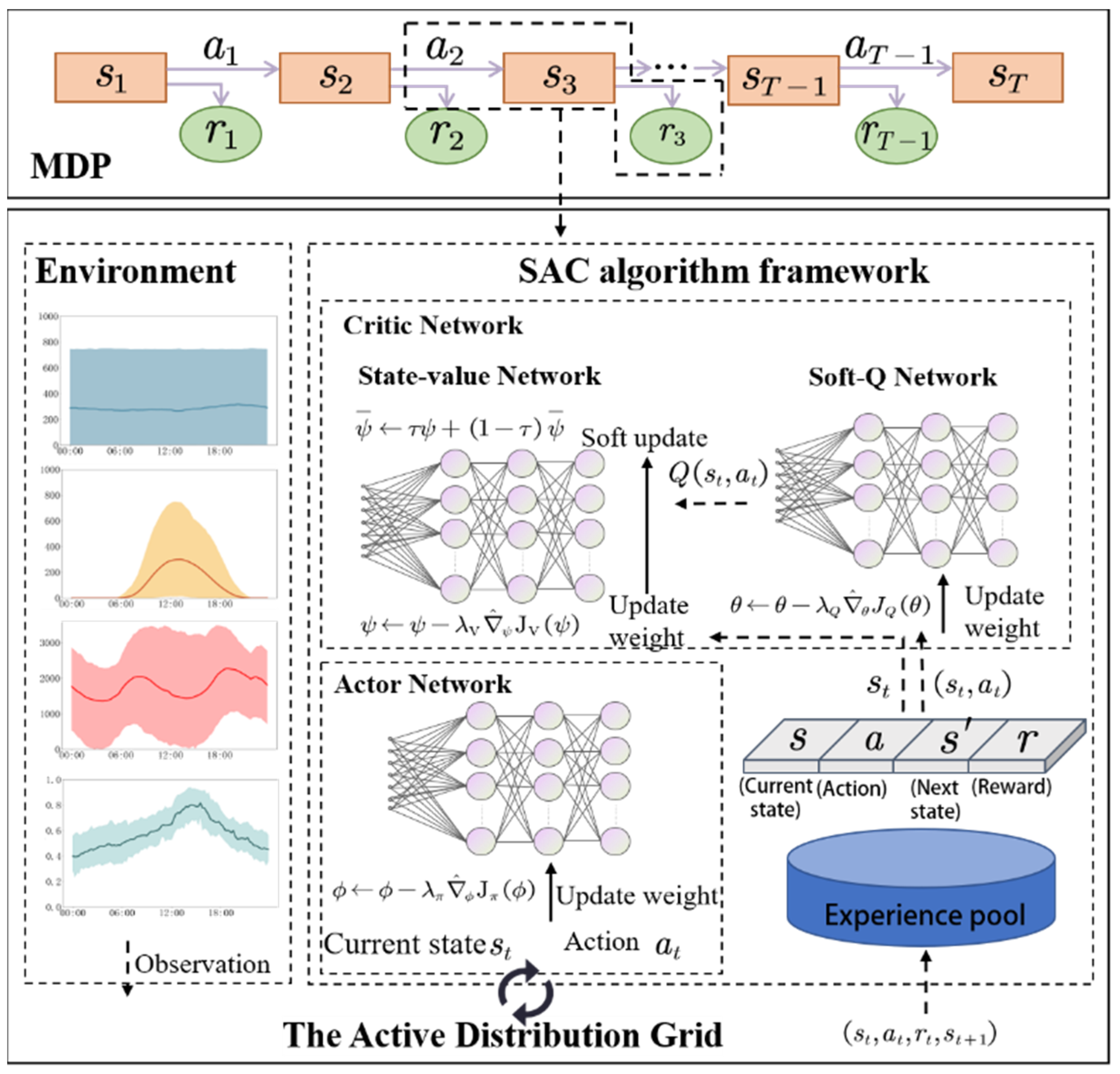
5.1. Markov Decision Process Framework

The low-carbon scheduling problem is a stochastic sequential decision-making problem, which requires continuous decision-making on the operation of gas units and energy storage devices with respect to the uncertainty conditions of new energy outputs, nodal loads, and carbon potentials of the main network in the distribution network.
We use Markov Decision Process (MDP) as a mathematical framework for modeling stochastic sequential decision-making problems, and model the dispatch model as an MDP framework with a finite time step according to the characteristics of the carbon potential calculation of the distribution network, which contains four elements ( S , A , p , r ):
(1)
S is the state space that supports all gas units and energy storage devices in the distribution network to make action decisions. The variables in the state space are all continuous values.
The observation state st is denoted as
s t = e Grid ( t ) , P Load N ( t ) , P WT K W ( t ) , P PV K F ( t ) , e Node K M ( t ) , e Node M ( t ) , P MT K M ( t 1 ) , S O C M ( t 1 )
The state contains variables such as the carbon potential eGrid(t) of the main grid, the load vector P Load N (t) of each node, the turbine power vector P WT K W (t), the PV power vector P PV K P (t), the carbon potential e Node K W (t) of the node to which the combustion turbine is connected, and the carbon potential e Node M (t) of the node to which the energy storage is connected, as well as the combustion turbine power P WT K W (t − 1) and the energy storage charge state SOCM(t − 1). Excluding the main network carbon potential, the rest of the vectors contain multiple state quantities; the superscript indicates the number of state quantities.
(2)
A is the action space. During the time period t, the intelligent body outputs the optimal action according to the environmental changes. The action at contains the unit output and the operating status of the energy storage device:
a t = P MT K M ( t ) , P ESS M ( t )
where P WT K W (t) denotes the active power of KM gas units at moment t and P ESS M (t) denotes the charging power or discharging power of M energy storage devices.
(3)
p is the state transfer probability, which denotes the probability density of the current state st to move to the next state st+1 under action at. The transition process from st to st+1 can be expressed as
s t + 1 = f trans s t , w t , P MT K M ( t ) , P ESS M ( t )
where P MT K M (t) and P ESS M (t) are the action values in the current state and wt denotes the environmental randomness.
(4)
r denotes the reward returned from the environment for taking action at during each round of state transfer:
r t ( s t , a t ) = - E T ( t )
where ET(t) is the single-step carbon emission cost during the dispatch cycle.

5.2. Improvement of Soft Actor–Critic Algorithm

In the actual operation situation, the environmental stochasticity makes it difficult to establish an accurate model; we propose the use of the improved Soft Actor–Critic (SAC) algorithm to solve the above MDP problem [29]. The overall structure is shown in Figure 4.
SAC uses one Actor Network and two Critic Networks to model strategies and value functions:
(1)
Actor Network
The Actor Network is used to decide the action that should be taken in a given state. It takes the current state as input, outputs the action and the corresponding policy entropy, and learns the optimal policy π * by maximizing the entropy objective, as shown in (29).
π * = arg   max π E [ t r ( s t , a t ) + α H ( π ( | s t ) ) ]
where E represents the expectation function, π * and π represent the optimal and current strategies, respectively, and px is the probability distribution corresponding to the state action under strategy π ; the entropy reward term H ( π ( | s t ) ) = a t π ( a t | s t ) log π ( a t | s t ) is used to increase the strategy diversity; and the weight of the entropy term in the overall reward function is adjusted by the temperature factor α.
To address the uncertainty of sustainable energy sources and loads in the operating environment of an ADN, we improve the reward function r t ( s t , a t ) of the SAC algorithm to improve the robustness of the model. In the reward function, the strategies that do not satisfy the constraints are penalized by the penalty term δ:
δ = δ 0 + δ DN + δ MT + δ ESS
δ DN = η DN ( Δ U max ( t ) Δ U max ) , Δ U max ( t ) > Δ U max 0 , Δ U max ( t ) Δ U max
δ MT = η MT ( p MT ( t ) p MT max ) , p MT ( t ) > p MT max 0 , p MT ( t ) p MT max
δ ESS = η ESS ( S O C ESS min S O C ( t ) ) , S O C ( t ) < S O C ESS min 0 , S O C ESS min S O C ( t ) S O C ESS max η ESS ( S O C ( t ) S O C ESS max ) , S O C ( t ) > S O C ESS max
where δ0 is the distribution network tidal current, security, and power balance constraint penalty term; δDN is the distribution network allowable voltage deviation value penalty term; δMT is the maximum output power penalty term for gas-fired units; δESS is the energy storage equipment charge state limitation penalty term; and η is the penalty coefficient.
At the same time, we consider that the objective used to evaluate the difference between the cost and the penalty is large, which affects the solution. In this paper, we use the reward function based on Gaussian distribution for each item, firstly, we calculate the target value ET and the penalty term δ of the current strategy according to Equations (16) and (30), and we select the corresponding standard deviation σ1 and σ2 according to the value domain, and since the target values are all positive, we take the mean value of Gaussian distribution to be 0 and obtain the improved reward function:
r ( s t , a t ) = λ 1 σ 1 2 π e E T 2 2 σ 1 2 + λ 2 σ 2 2 π e δ 2 2 σ 2 2
where λ1 and λ2 are the respective adjustable weight coefficients used to modulate the effects of the two Gaussian distributions.
Then, the update of the optimization objective function and the temperature parameter α in the Actor Network is expressed as
J π ϕ = E s t ~ D α log π ϕ f ϕ ϵ t ; s t s t Q θ s t , f ϕ ϵ t ; s t
J π ( α ) = E s t ~ D , a t π t [ α ln π ( a t | s t ) α H 0 ]
where D is the experience pool; f ϕ ( ϵ t ; s t ) is the Actor Network; ϕ is the network parameters; H0 is the dimension of the action matrix.
(2)
Critic Networks
The core task of the Critic Networks is to learn and approximate a state-action value function Q ( s t , a t ) to evaluate the expected reward of the current policy for taking a given action in a given state. SAC uses two independent Critic Networks to implement this function, reducing the overestimation bias in the estimation of the Q-value and improving the stability of the algorithm. The Q-value y is calculated by the current reward r t and the Q-value of the next state to be computed:
y = r t + γ min ( Q θ 1 ( s t + 1 , a t + 1 ) , Q θ 2 ( s t + 1 , a t + 1 ) ) α log π ϕ ( a t + 1 | s t + 1 )
where γ is the discount factor, which measures the importance of future rewards; Q θ 1 and Q θ 2 are the target Q networks, which are used to compute the Q-value for the next state; α is the temperature parameter; and log π ϕ ( a t + 1 | s t + 1 ) is the logarithmic probability that the strategy network will choose action at+1 in the next state.
The loss function J Q ( θ i ) of each Critic Network i is achieved by minimizing the mean square error between the target Q-value and the predicted Q-value:
J Q ( θ i ) = E ( s i , a i , r i , s i + 1 ) ~ D 1 2 ( Q θ i ( s t , a t ) y ) 2
where D is the experience pool, storing previous state transfer samples; θi is a parameter of the Critic Network Q θ i . The agent training process is shown in Algorithm 1.
In each step of the decision-making process, the intelligent agent firstly carries out ADN power flow calculation and carbon flow calculation according to the node load changes and the power changes of sustainable energy sources to obtain the distribution of the node carbon potential of the node that has not been connected to the power generation equipment and updates the state space variables. Subsequently, decision-making actions are made based on the state information of load and carbon potential in the state space, in which, according to the analysis of the dynamic impact of distributed power on node carbon potential in Section 2.2, the carbon potential state of the node is an important basis for influencing the action decision. Subsequently, it judges whether the constraints are satisfied, calculates the reward value, and completes the decision-making of a dispatch cycle.
Algorithm 1 Solving dispatch model based on improved SAC
1: Initialize:
    Policy network πϕ
    Two Q networks Q θ 1 and Q θ 2 .
    Target Q networks Q θ 1 and Q θ 2 .
    Replay buffer D .
2: for each environment step do:
3:     Sample action at∼πϕ(⋅∣st) from the policy at state st.
4:     Execute action at, receive reward r t and next state st+1.
5:     Store transition (st, at, r t , st+1) in D .
end for
6: for each update step do:
7:     Randomly sample a batch of transitions (st, at, r t , st+1) from D .
8:     Compute target value according to Equation (37).
9:     Update critic networks according to Equation (38):
θ i θ i θ i J Q ( θ i )
10:   Update policy network according to Equation (35):
ϕ ϕ ϕ J π ( ϕ )
11:   Adjust temperature parameter α according to Equation (36):
α α α J ( α )
12: Update target Q networks:
θ i τ θ i + ( 1 τ ) θ i
end for
13: Output: Learned policy network parameters
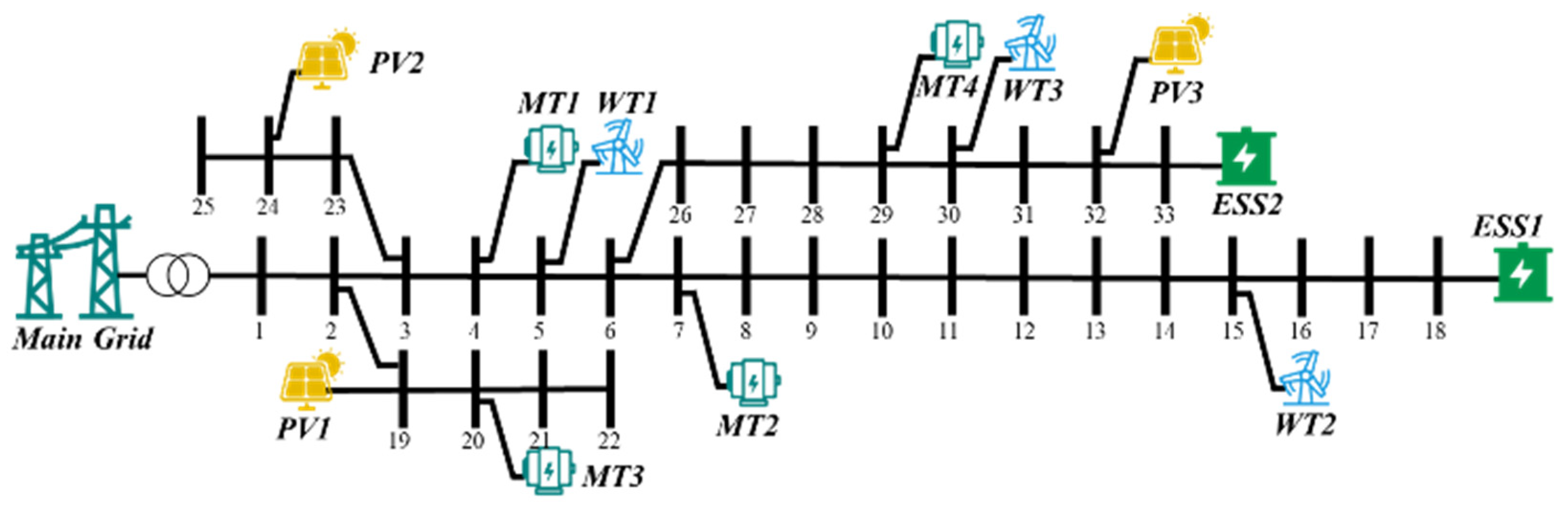
6. Case Simulation

6.1. Experimental Configuration

In order to validate the effectiveness and advantages of the low-carbon dispatch methodology proposed in this paper for active distribution networks, it is validated on a modified IEEE 33-bus system. The node system is shown in Figure 5, with WTs at nodes 5, 15, and 30, photovoltaic arrays at nodes 19, 24, and 32, dispatchable gas-fired units at nodes 4, 11, and 29, and electrical energy storage devices at nodes 18 and 33. The operating parameters of the devices are shown in Table 1.
The wind power generation, PV generation data, load data, and main grid carbon potential change data in distribution network operation are obtained from Tianjin, China, with a sampling interval of 15 min. The dataset is subjected to data cleansing, and the data in the dataset are scaled to the corresponding level of the IEEE 33-node data.
The hyperparameter configuration of the SAC network parameter training process is shown in Table 2.
The training of all models in this paper was deployed in a Python 3.6.9 environment under a Windows 11 operating system with computer hardware configurations of CPU: AMD Ryzen 7 4800H and GPU: RTX 3060.

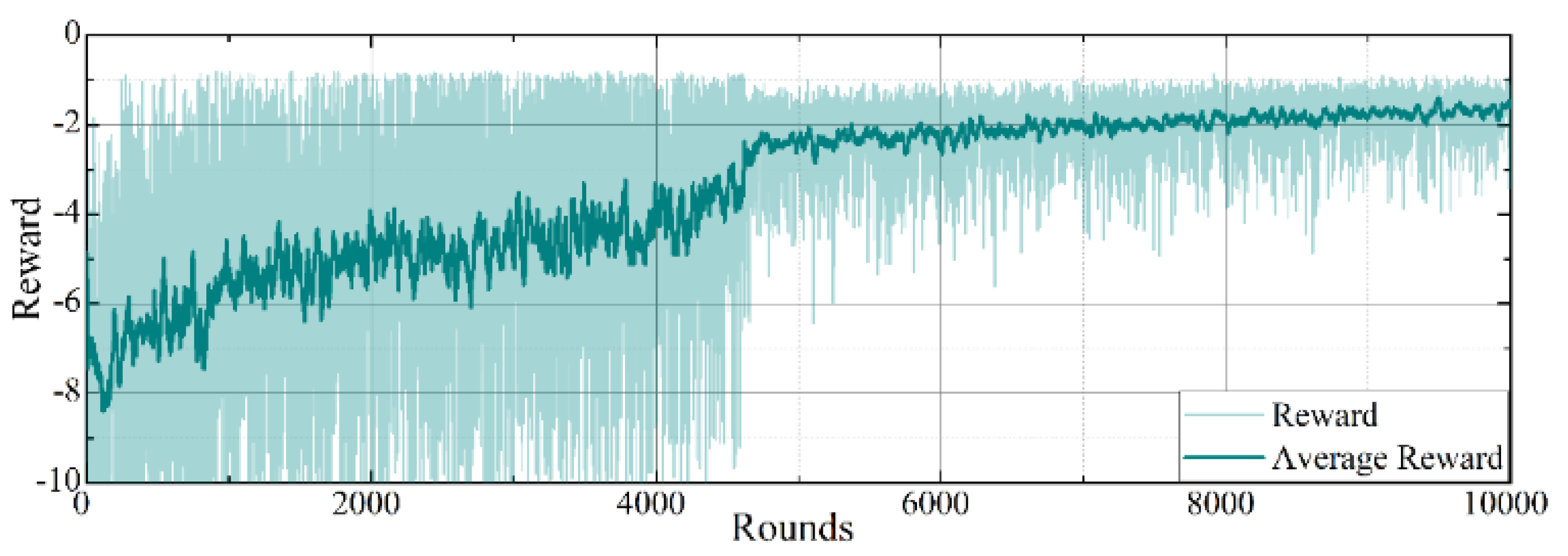
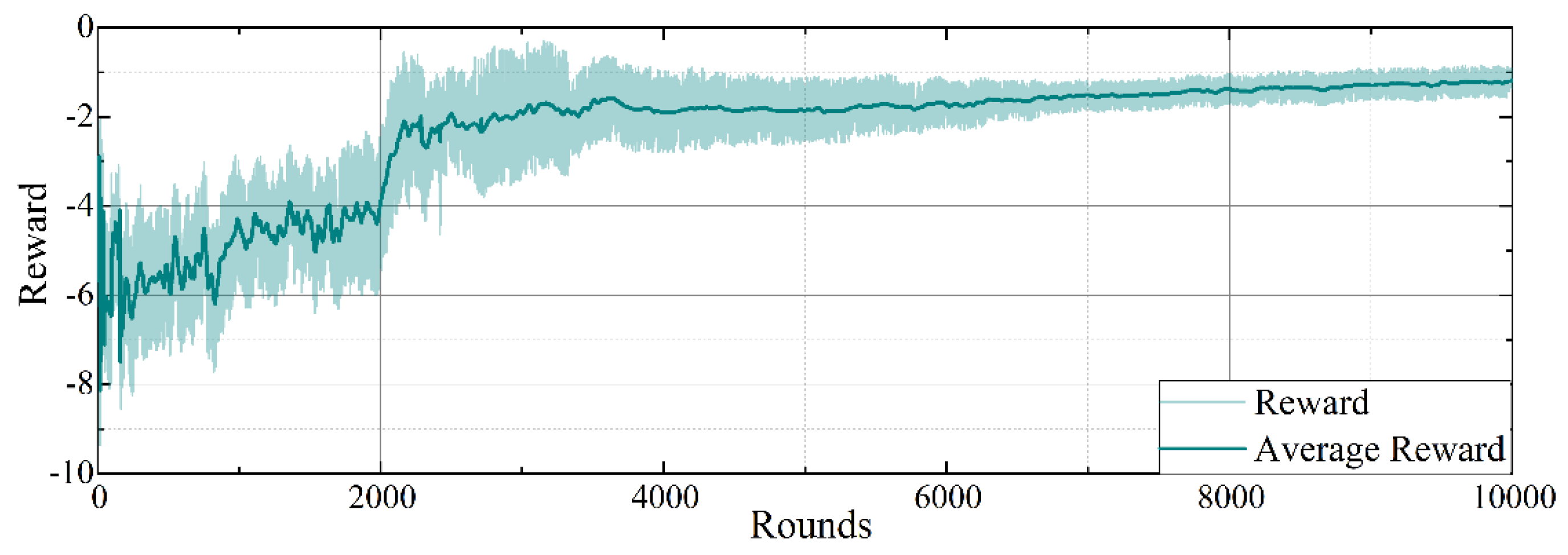
6.2. Evaluation of the Training Process

The convergence trend of the average reward curve obtained during training is an important indicator for evaluating the performance of deep reinforcement learning algorithms. Figure 6 shows the training process curves of the intelligence using the original reward function in 10,000 rounds of training. We use the linear sum of the objective function and the normalized penalty term as the original reward function. Meanwhile, the change curve of the reward value of the improved algorithm proposed in this paper is shown in Figure 7.
The intelligent body achieves high stochasticity exploration through the maximum entropy strategy in the initial stage, and most of the decisions will deviate from the optimization objective, so the reward curve shows a large change. As the training process continues, the interaction between the intelligent body and the operating environment of the distribution network becomes more obvious, the reward value gradually rises, and finally, the reward curve converges to a certain high value at the end of the training, indicating that the intelligent body learns the optimal dispatch strategy to realize the multi-objective. Compared with the simple linear combination of reward functions, the reward curve of the method improved with Gaussian distribution fluctuates less, indicating that the algorithm is more stable, and at the same time the rewards converge at about 2200 rounds, which is faster compared to the control group method that converges at about 4600 rounds. Thus, the improved reward function algorithm using Gaussian sampling outperforms the normal algorithm for most of the training time.

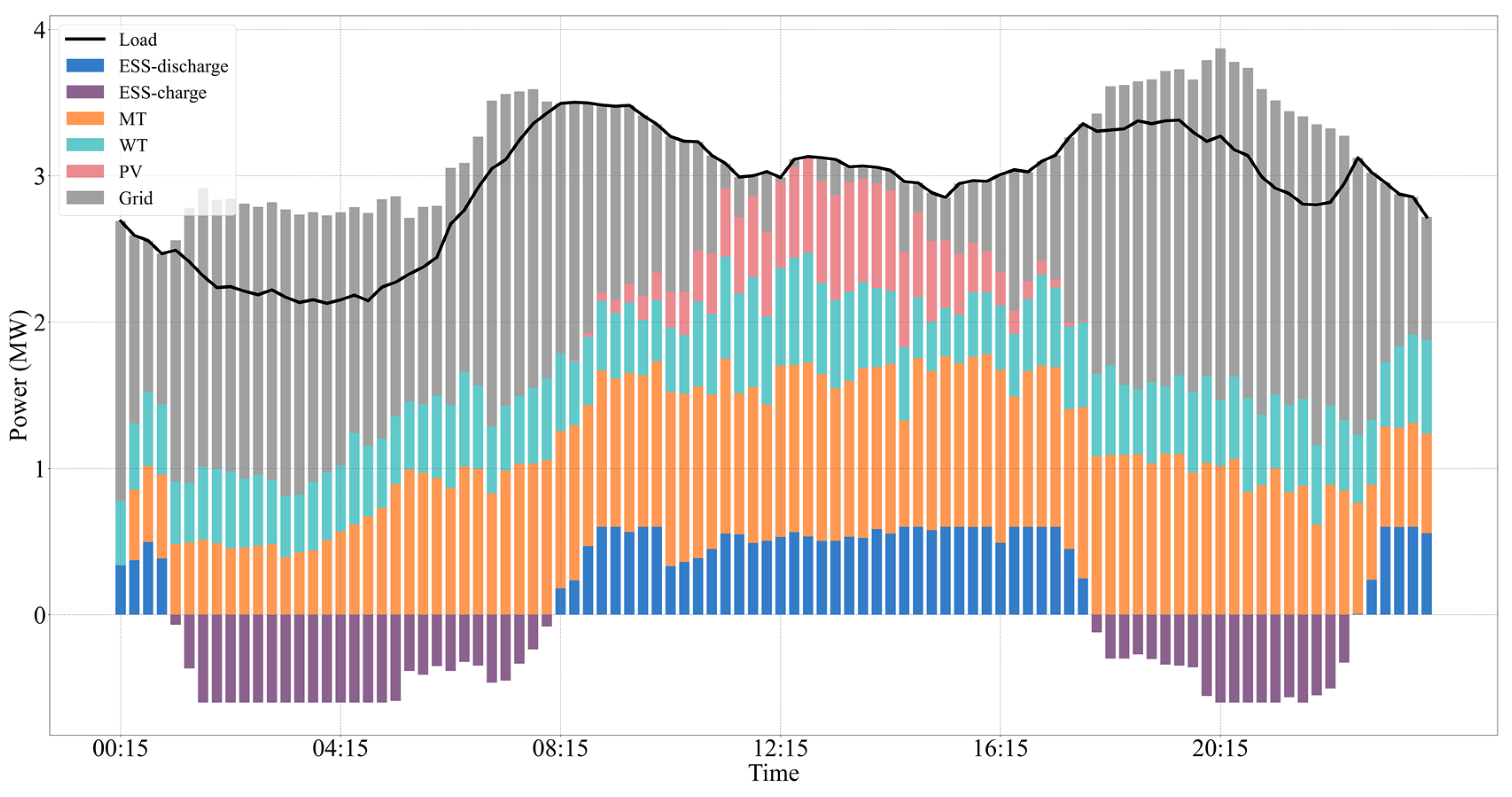
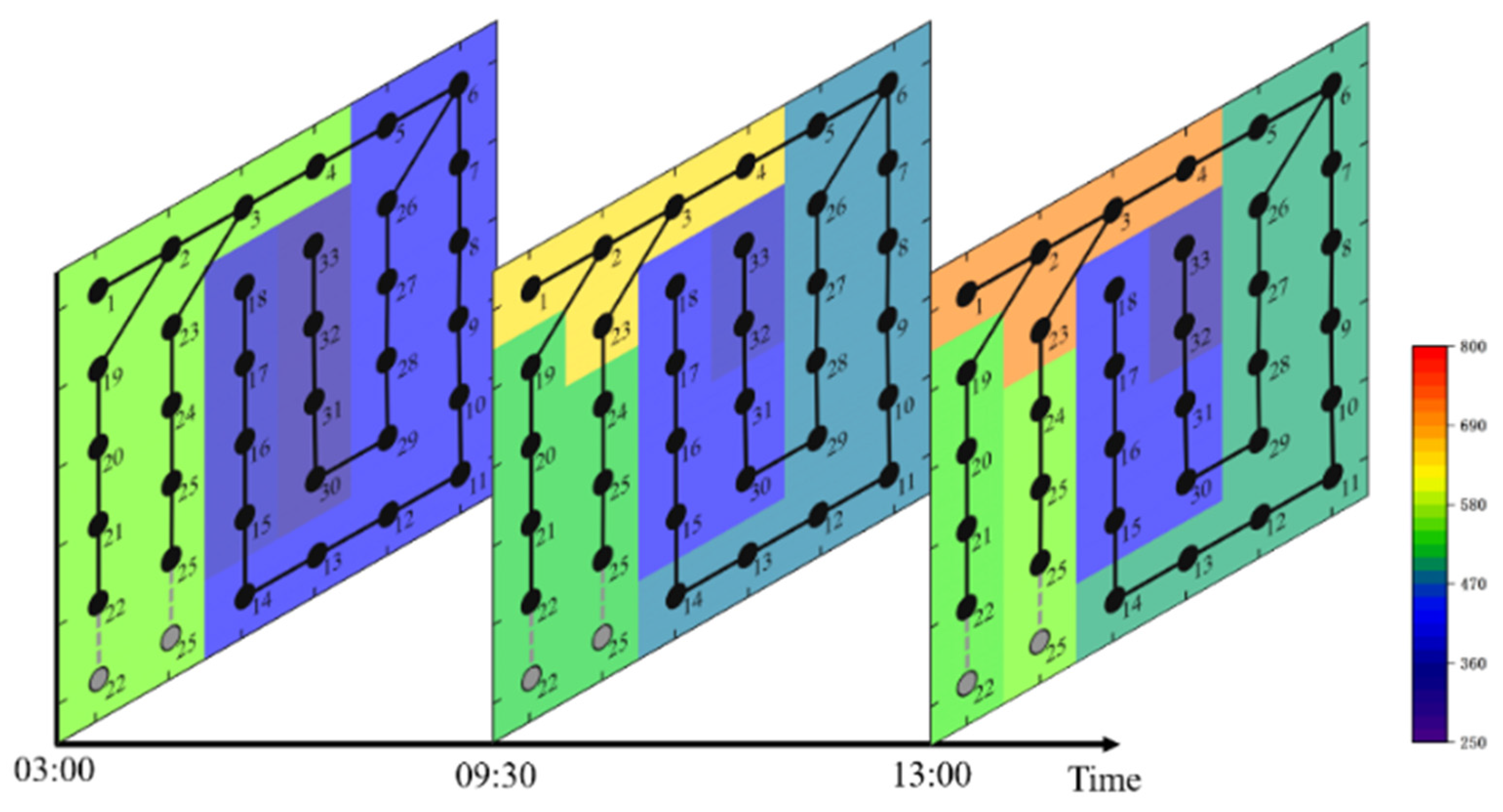
6.3. Scheduling Result Performance

The intelligent body trained using the training set dataset is capable of realizing real-time optimal scheduling of the active distribution network, in order to verify the performance of the improved SAC algorithm, the data of one scheduling cycle (24 h) are selected in the test set to evaluate the scheduling of each device in the operation of the active distribution network, as well as the changes in the distribution network indices.
From Figure 8, it can be seen that the gas unit and energy storage equipment in the ADN act according to the carbon potential of the main grid, the power output of wind and solar sustainable energy, and load changes. In the low power consumption time, such as 1:15–6:00, the carbon potential of the main grid is at a low level, the gas unit reduces the power output, the energy storage equipment is in a charging state, and the distribution network increases the low-carbon power input from the main grid. During peak hours, such as 16:30–18:30, when the carbon potential of the main grid is at a higher level, the distribution network is controlled to increase the output power of the gas-fired units, and the energy storage equipment is discharged to output the clean power stored during the low carbon potential hours, so as to reduce the use of high carbon power in the main grid.
The change in the operating status of 1# gas unit under the change in carbon potential of the main grid is shown in Figure 9. When the carbon potential of the main grid is lower than the carbon emission factor of the gas unit, such as during the 0:00–7:00 time period, the output power of the gas unit is lower, mainly playing the role of regulating the stable operation of the distribution network. When the carbon potential of the main grid is higher than the carbon emission factor of the gas-fired units, such as during the 10:00–17:00 time period, the gas-fired units are used to replace part of the main grid power input, and at this time, under the fixed load and storage demand, the gas-fired units have a better low-carbon benefit compared with the main grid transmission of the same amount of electricity, and thus the unit output power increases.
Figure 10 shows the scheduling results of 1# energy storage equipment under the change in carbon potential of its connected 3# node, setting the initial 2 of the energy storage equipment as 80%, and the initial carbon flow rate as 0.6 kgCO2/kWh. In the initial stage, the energy storage equipment discharges continuously in order to respond to the high load demand of the distribution network, and when the load demand decreases, and the node carbon potential is lower than the carbon emission factor of the energy storage equipment, such as in the time period from 1:45 to 7:30, the energy storage equipment changes to charging state and absorbs the low-carbon power from the distribution network, and its discharge carbon emission factor is calculated to be 0.57 kgCO2/kWh at the end of the charging state based on the changes in the nodal carbon potential and charging power in the model of Equation (9). When the load demand increases, such as 7:45–17:30, the energy storage device continuously discharges and outputs the low-carbon power stored in the previous charging state, and the carbon emission factor of the discharge is 0.57 kgCO2/kWh, which is lower than the node carbon potential, thus realizing the effect of reducing carbon emissions.
The 33-node distribution network is plotted as a 6 × 6 grid diagram, which represents the distribution of nodal carbon potential at a certain moment in time, and the color represents the numerical level of nodal carbon potential. Figure 11 shows the distribution of nodal carbon potential at different times of the distribution network without considering the dispatch of gas units and energy storage devices. Figure 12 shows the distribution of carbon potential in different time periods using the proposed model and the optimal operation strategy. Comparing the two figures, it can be intuitively seen that this method reduces the overall carbon potential during active distribution network operation, expands the radiation range of zero-carbon emission energy sources such as wind and photovoltaic, and improves the utilization rate by controlling gas-fired units and energy storage devices in response to the new energy output and the high carbon and low carbon changes in the main network.
In summary, under the multivariate changes in carbon potential, wind power, and load in the active distribution network, the intelligent agent trained by using the improved SAC algorithm can control the operating state of gas units and energy storage devices in the distribution network, reduce the output of gas units and increase the charging power of energy storage devices to absorb low-carbon power during the low-carbon time of the main network, and increase the output of gas units and control the release of stored low-carbon power from energy storage devices during the high-carbon time of the main network. During the high-carbon hours of the main grid, it increases the output of gas units and controls the energy storage equipment to release the stored low-carbon power, so as to realize the low-carbon operation of the distribution network and meet the load supply and stable operation.

6.4. Comparison of Model-Solving Algorithms

Under the hyperparameter configuration of Table 2, the improved SAC algorithm proposed in this paper is compared with the classical SAC, DDPG [30], and PPO [31] algorithms, and the results of carbon emission cost comparison are shown in Table 3.
The DDPG method defines two neural networks: one for the policy (Actor) and one for the value function (Critic), similar to the SAC method discussed in this paper. It uses an experience replay buffer to store the agent’s experiences, allowing for random sampling during training to break data correlation. PPO includes a shared main network for generating policies and estimating value functions. It optimizes the objective function through gradient ascent to update the network parameters, facilitating the learning of the agent.
The improved SAC algorithm used in this paper utilizes a Gaussian distribution reward function, which is able to converge to the optimal solution faster, and reduces carbon emissions by 6.4% compared to the classical SAC algorithm. Compared to the PPO, which requires massive data training, and the DDPG algorithm, which adopts a deterministic policy, the carbon emissions of the methods used in this paper are reduced by 7% and 12.7%, respectively, to realize the optimal operation of the active distribution network low carbon scheduling model proposed in this paper.

7. Conclusions

In this paper, a model and method for low-carbon scheduling of active distribution networks combining carbon flow calculation theory and deep reinforcement learning are constructed. By establishing the operation model and carbon flow calculation model of lossy distribution networks, we realize the carbon measurement of each operational link, and based on this, we establish the active low-carbon dispatch model of the distribution network taking into account the wind and solar intermittent energy, so as to make the carbon emission cost of the operation of the distribution network have a better explanation, and the calculation of the node carbon potential provides support for the optimal decision-making of the combustion turbine and the energy storage equipment. The powerful data fitting and decision-making ability of deep reinforcement learning is utilized to solve the optimal operation strategy, and the method of using the combination of Gaussian distributions is improved on the basis of the classical SAC algorithm, which significantly improves the training effect of the intelligent agent. Finally, in the arithmetic test, the intelligent body is able to make decisions based on the real-time measured demand load, wind and solar output, and carbon potential data of the main network without any prediction information, which improves the adaptability of the system to uncertainty and verifies the effectiveness of the model and algorithm improvement in this paper.

Author Contributions

Conceptualization, J.B. and T.Y.; methodology, Z.D.; validation, J.B. and T.Y. and Z.D.; formal analysis, Z.D.; investigation, Z.D.; resources, J.B. and Y.W.; data curation, Y.W., T.X. and Z.G.; writing—original draft preparation, Z.D.; writing—review and editing, Z.D. and T.Y.; visualization, Z.D.; supervision, T.Y.; project administration, J.B., T.X. and Z.G.; funding acquisition, J.B., T.X. and Z.G. All authors have read and agreed to the published version of the manuscript.

Funding

This paper is supported by the Science and Technology Project of State Grid Tianjin Electric Power Company “Research on Key Technology of Carbon Emission Accounting and Carbon Monitoring and Calibration of New Electric Power System Based on Energy and Electric Power Big Data and Carbon Emission Trend Analysis Technology for Mega Cities” under Grant DK-YF2023-46.

Data Availability Statement

Not available due to data privacy.

Conflicts of Interest

Authors Jiang Bian and Zhiyong Gan were employed by the company Electric Power Science Research Institute, State Grid Tianjin Electric Power Company. Authors Yang Wang and Tianchun Xiang were employed by the company State Grid Tianjin Electric Power Company. The authors declare that this study received funding from State Grid Tianjin Electric Power Company. The funder was not involved in the study design, collection, analysis, interpretation of data, the writing of this article or the decision to submit it for publication. The remaining authors declare that the research was conducted in the absence of any commercial or financial relationships that could be construed as a potential conflict of interest.

References

  1. Nakhli, M.S.; Shahbaz, M.; Jebli, M.B.; Wang, S. Nexus between economic policy uncertainty, renewable & non-renewable energy and carbon emissions: Contextual evidence in carbon neutrality dream of USA. Renew. Energy 2022, 185, 75–85. [Google Scholar]
  2. Scarlat, N.; Prussi, M.; Padella, M. Quantification of the carbon intensity of electricity produced and used in Europe. Appl. Energy 2022, 305, 117901. [Google Scholar] [CrossRef]
  3. Zhao, G.; Yu, B.; An, R.; Wu, Y.; Zhao, Z. Energy system transformations and carbon emission mitigation for China to achieve global 2 C climate target. J. Environ. Manag. 2021, 292, 112721. [Google Scholar] [CrossRef] [PubMed]
  4. Chilvers, J.; Bellamy, R.; Pallett, H.; Hargreaves, T. A systemic approach to mapping participation with low-carbon energy transitions. Nat. Energy 2021, 6, 250–259. [Google Scholar] [CrossRef]
  5. Gu, C.; Liu, Y.; Wang, J.; Li, Q.; Wu, L. Carbon-oriented planning of distributed generation and energy storage assets in power distribution network with hydrogen-based microgrids. IEEE Trans. Sustain. Energy 2022, 14, 790–802. [Google Scholar] [CrossRef]
  6. Xu, W.; Yu, B.; Song, Q.; Weng, L.; Luo, M.; Zhang, F. Economic and low-carbon-oriented distribution network planning considering the uncertainties of photovoltaic generation and load demand to achieve their reliability. Energies 2022, 15, 9639. [Google Scholar] [CrossRef]
  7. Chen, S.; Liu, Y.; Guo, Z.; Luo, H.; Zhou, Y.; Qiu, Y.; Zhou, B.; Zang, T. Deep reinforcement learning based research on low-carbon scheduling with distribution network schedulable resources. IET Gener. Transm. Distrib. 2023, 17, 2289–2300. [Google Scholar] [CrossRef]
  8. Qing, Y.; Liu, T.; He, C.; Nan, L.; Dong, G.; Gao, W.; Yu, Y. Low-carbon coordinated scheduling of integrated electricity-gas distribution system with hybrid AC/DC network. IET Renew. Power Gener. 2022, 16, 2566–2578. [Google Scholar] [CrossRef]
  9. Chen, L.; Zhou, Y. Low carbon economic scheduling of residential distribution network based on multi-dimensional network integration. Energy Rep. 2023, 9, 438–448. [Google Scholar] [CrossRef]
  10. Li, B.; Song, Y.; Hu, Z. Carbon flow tracing method for assessment of demand side carbon emissions obligation. IEEE Trans. Sustain. Energy 2013, 4, 1100–1107. [Google Scholar] [CrossRef]
  11. Kang, C.; Zhou, T.; Chen, Q.; Xu, Q.; Xia, Q.; Ji, Z. Carbon emission flow in networks. Sci. Rep. 2012, 2, 479. [Google Scholar] [CrossRef] [PubMed]
  12. Kang, C.; Zhou, T.; Chen, Q.; Wang, J.; Sun, Y.; Xia, Q.; Yan, H. Carbon emission flow from generation to demand: A network-based model. IEEE Trans. Smart Grid 2015, 6, 2386–2394. [Google Scholar] [CrossRef]
  13. Notton, G.; Nivet, M.L.; Voyant, C.; Paoli, C.; Darras, C.; Motte, F.; Fouilloy, A. Intermittent and stochastic character of renewable energy sources: Consequences, cost of intermittence and benefit of forecasting. Renew. Sustain. Energy Rev. 2018, 87, 96–105. [Google Scholar] [CrossRef]
  14. Notton, G.; Nivet, M.L.; Voyant, C.; Paoli, C.; Darras, C.; Motte, F.; Fouilloy, A. Enhancing smart grid integrated renewable distributed generation capacities: Implications for sustainable energy transformation. Sustain. Energy Technol. Assess. 2024, 66, 103793. [Google Scholar]
  15. Dashtaki, A.A.; Hakimi, S.M.; Hasankhani, A.; Derakhshani, G.; Abdi, B. Optimal management algorithm of microgrid connected to the distribution network considering renewable energy system uncertainties. Int. J. Electr. Power Energy Syst. 2023, 145, 108633. [Google Scholar] [CrossRef]
  16. Zhao, C.; Qin, X.; Wang, A.; Song, R.; Zhou, W.; Sun, Z. Design of photovoltaic-energy storage-load forecasting and optimal control method for distributed distribution network based on reinforcement learning. In Proceedings of the Ninth International Conference on Energy Materials and Electrical Engineering (ICEMEE 2023), Guilin, China, 25–27 August 2023; SPIE: Bellingham, WA, USA, 2024; Volume 12979, pp. 902–907. [Google Scholar]
  17. Zhang, X.; Wu, Z.; Sun, Q.; Gu, W.; Zheng, S.; Zhao, J. Application and progress of artificial intelligence technology in the field of distribution network voltage Control: A review. Renew. Sustain. Energy Rev. 2024, 192, 114282. [Google Scholar] [CrossRef]
  18. Yang, T.; Zhao, L.Y.; Liu, Y.; Feng, S.; Pen, H. Dynamic Economic Dispatch for Integrated Energy System Based on Deep Reinforcement Learning. Autom. Electr. Power Syst. 2021, 45, 39–47. (In Chinese) [Google Scholar]
  19. Li, Y. Deep reinforcement learning: An overview. arXiv 2017, arXiv:1701.07274. [Google Scholar]
  20. Cao, D.; Hu, W.; Xu, X.; Wu, Q.; Huang, Q.; Chen, Z.; Blaabjerg, F. Deep reinforcement learning based approach for optimal power flow of distribution networks embedded with renewable energy and storage devices. J. Mod. Power Syst. Clean Energy 2021, 9, 1101–1110. [Google Scholar] [CrossRef]
  21. Hosseini, M.M.; Parvania, M. On the feasibility guarantees of deep reinforcement learning solutions for distribution system operation. IEEE Trans. Smart Grid 2023, 14, 954–964. [Google Scholar] [CrossRef]
  22. Xing, Q.; Chen, Z.; Zhang, T.; Li, X.; Sun, K. Real-time optimal scheduling for active distribution networks: A graph reinforcement learning method. Int. J. Electr. Power Energy Syst. 2023, 145, 108637. [Google Scholar] [CrossRef]
  23. Lu, Y.; Xiang, Y.; Huang, Y.; Yu, B.; Weng, L.; Liu, J. Deep reinforcement learning based optimal scheduling of active distribution system considering distributed generation, energy storage and flexible load. Energy 2023, 271, 127087. [Google Scholar] [CrossRef]
  24. Xu, D.; Wu, Q.; Zhou, B.; Li, C.; Bai, L.; Huang, S. Distributed Multi-Energy Operation of Coupled Electricity, Heating, and Natural Gas Networks. IEEE Trans. Sustain. Energy 2019, 11, 2457–2469. [Google Scholar] [CrossRef]
  25. Ibrahim, H.; Ilinca, A.; Perron, J. Energy storage systems—Characteristics and comparisons. Renew. Sustain. Energy Rev. 2008, 12, 1221–1250. [Google Scholar] [CrossRef]
  26. Zhou, T.; Kang, C.; Xu, Q.; Chen, Q. Preliminary Investigation on a Method for Carbon Emission Flow Calculation of Power System. Autom. Electr. Power Syst. 2012, 36, 44–49. (In Chinese) [Google Scholar]
  27. Shirmohammadi, D.; Hong, H.W. Reconfiguration of electric distribution networks for resistive line losses reduction. IEEE Trans. Power Deliv. 1989, 4, 1492–1498. [Google Scholar] [CrossRef]
  28. Gupta, N.; Swarnkar, A.; Niazi, K.R. Distribution network reconfiguration for power quality and reliability improvement using Genetic Algorithms. Int. J. Electr. Power Energy Syst. 2014, 54, 664–671. [Google Scholar] [CrossRef]
  29. Haarnoja, T.; Zhou, A.; Hartikainen, K.; Tucker, G.; Ha, S.; Tan, J.; Kumar, V.; Zhu, H.; Gupta, A.; Abbeel, P.; et al. Soft actor-critic algorithms and applications. arXiv 2018, arXiv:1812.05905. [Google Scholar]
  30. Silver, D.; Lever, G.; Heess, N.; Degris, T.; Wierstra, D.; Riedmiller, M. Deterministic policy gradient algorithms. In Proceedings of the International Conference on Machine Learning, PMLR, Beijing, China, 22–24 June 2014; pp. 387–395. [Google Scholar]
  31. Schulman, J.; Wolski, F.; Dhariwal, P.; Radford, A.; Klimov, O. Proximal policy optimization algorithms. arXiv 2017, arXiv:1707.06347. [Google Scholar]
Figure 1. Schematic diagram of the ADN and its carbon flow distribution.
Energies 17 05610 g001
Figure 2. Schematic diagram of the lossless network equivalent process.
Energies 17 05610 g002
Figure 3. Schematic diagram of carbon reduction of power generation equipment.
Energies 17 05610 g003
Figure 4. Improved SAC algorithm structure.
Energies 17 05610 g004
Figure 5. Sample topology of 33-node distribution network operation.
Energies 17 05610 g005
Figure 6. Change curve of intelligent agent training reward for control group.
Energies 17 05610 g006
Figure 7. Intelligent agent training reward change curve for proposed method.
Energies 17 05610 g007
Figure 8. Test day electric power dispatch results.
Energies 17 05610 g008
Figure 9. Operation of 1# gas-fired unit under the change in carbon potential of the main network.
Energies 17 05610 g009
Figure 10. Results of energy storage device operation under carbon potential change at the connected node.
Energies 17 05610 g010
Figure 11. Distribution of carbon potential at distribution network nodes for different time periods.
Energies 17 05610 g011
Figure 12. Distribution of carbon potential at distribution network nodes for the proposed method.
Energies 17 05610 g012
Table 1. Units running parameters.
TypeParametersValue
Wind power units P WT max 250 kW
Photovoltaic array P WT max 250 kW
Gas units p MT max 300 kW
p MT down / p MT up −60/60 kW/15 min
Energy storage devices η ESS 0.85
p ESS min / p ESS max −300/300 kW
S O C ESS min 20%
S O C ESS max 85%
Ncycle8000
The main net Δ U max 7%
Table 2. Training hyperparameter setting of sac model.
ParametersValue
Learning rate of Actor1 × 10−5
Learning rate of Critic1 × 10−5
Decay ratio of learning rate0.5
Batch size256
Epoch10,000
Discount factor0.97
Parameter update speed0.01
Temperature parameter0.01
Buffer size1 × 104
Buffer initial fill2560
Updates frequency 10
Table 3. Comparative results of carbon emission costs of different algorithms.
MethodProposed MethodSACPPODDPG
Carbon Emission (kgCO2)50,32553,74954,05157,668
Disclaimer/Publisher’s Note: The statements, opinions and data contained in all publications are solely those of the individual author(s) and contributor(s) and not of MDPI and/or the editor(s). MDPI and/or the editor(s) disclaim responsibility for any injury to people or property resulting from any ideas, methods, instructions or products referred to in the content.

