Adaptive Remaining Capacity Estimator of Lithium-Ion Battery Using Genetic Algorithm-Tuned Random Forest Regressor Under Dynamic Thermal and Operational Environments

Abstract

The increasing interests and recent advancements in artificial intelligence and machine learning have significantly accelerated the development of novel techniques for the state estimation of batteries in electrified vehicles’ battery management systems (BMSs). Determining the remaining capacity among the several BMS states is crucial for ensuring the safe and stable functioning of an electric vehicle. This paper proposes an adaptive estimator for the remaining capacity of lithium-ion batteries, leveraging a Genetic Algorithm (GA)-tuned random forest (RF) regressor. The estimator is designed to function effectively under varying thermal conditions. The optimization of critical parameters, namely, the number of estimators (n-estimators) and the minimum number of samples per leaf (min-samples-leaf), is a focal point of this study to enhance model accuracy and robustness. The model effectively captures the battery’s dynamic behavior and inherent non-linearity. The Mean Absolute Error (MAE) and Root Mean Square Error (RMSE) achieved during testing demonstrate promising accuracy and superior prediction. The results demonstrated significant improvements in state of charge (SOC) estimation accuracy. The proposed GA-optimized RF model achieved an MAE of 0.0026 at 25 °C and 0.0102 at −20 °C, showing a 41.37% to 50% reduction in the MAE compared to traditional random forest models without GA optimization. The RMSE was also reduced by 18.57% to 31.01% across the tested temperature range. These improvements highlight the model’s ability to accurately estimate the SOC in varying thermal conditions.

1. Introduction

1.1. Background and Overview of SOC Estimation

Advancements in ground-based transportation are critically needed due to the shortage of fossil fuels, rising demand for personal mobility, pollution emissions, and global warming. According to the Global EV Outlook, despite market obstacles and unfavorable attitudes towards electric vehicles (EVs), sales of electric cars are expected to increase globally. According to the projection, 17 million electric cars will be sold this year, with more than 20% of all automobiles sold worldwide, or more than one in five, being electric [1]. For the past decade, lithium-ion batteries have been a focus of research in both industry and academia due to their high cost in electric vehicles. Because of their slower self-discharge rate, improved energy density, and power efficiency, batteries in EVs require more affordable designs to offset their high initial costs [2,3].

Machine learning is used in a wide range of applications that include cybersecurity, EVs, and smart grid systems by strengthening threat detection, ensuring the system optimizes energy management and works as it should in terms of efficiency [4]. The battery management system (BMS) is crucial for overseeing individual battery cells within a battery pack. It monitors current and SOC imbalances, enabling real-time adjustments to enhance performance [5].

The innovative technologies for battery state estimation pursued inside the BMS of electrified vehicles have been considerably advanced by the growing demand and recent advances in artificial intelligence and machine learning thought, consequently improving their performance and operational efficiency. To ensure the safe and reliable operation of an electric vehicle, it is essential to determine the SOC among the battery’s numerous states [6]. The SOC is determined by comparing its residual capacity (Q_t) to its nominal capacity (Q_n). The SOC has a mathematical definition found in Equation (1).

$$\mathrm{SOC}={\displaystyle \frac{Q_t}{Q_n}}\times 100\%$$

(1)

Traditional methods for SOC estimation, such as the ampere-hour integration method (Coulomb counting) and open-circuit voltage (OCV) method, are straightforward and widely used. The Coulomb counting method tracks the charge and discharge currents over time; however, it can accumulate errors due to inaccuracies in the initial SOC and does not account for self-discharge or temperature effects. Similarly, the OCV method relies on a measured voltage at rest to estimate the SOC but requires rest periods and is affected by temperature and aging factors [7]. In contrast, model-based methods utilize mathematical models to describe battery dynamics, such as Equivalent Circuit Models (ECMs) and Electrochemical Models (EMs). While ECMs can yield accurate SOC estimates and are suitable for use with filtering algorithms, they require extensive testing for parameterization, leading to computational complexity. EMs provide high accuracy due to their detailed representation but are challenging to implement in real-time applications due to their complexity [8,9]. Filter-based methods, notably the Extended Kalman Filter (EKF) and Particle Filter (PF), enhance the robustness of SOC estimation by combining models with iterative estimation processes. The EKF effectively handles non-linearities and uncertainties in battery models but may be computationally intensive, thus limiting its use in low-power embedded systems. On the other hand, the PF handles non-linearities and non-Gaussian noise but it demands significant computational resources and memory [10,11]. Collectively, while the various SOC estimation methods offer distinct advantages, they also possess limitations that can affect their practical implementation, highlighting the need for advanced approaches to improve accuracy and reliability in battery management systems. Several challenges remain in the accurate estimation of the SOC, especially in dynamic environments, such as electric vehicle operation.

• Temperature Sensitivity: Temperature significantly affects battery performance and SOC estimation. Many SOC estimation models struggle to adapt to varying thermal conditions. Although techniques like PFs and KF have been used to account for these variations, they remain computationally intensive, making them difficult to deploy in low-power embedded systems.
• Battery Aging: As batteries age, their capacity degrades, which impacts SOC accuracy. Most estimation techniques assume a fixed nominal capacity, leading to inaccuracies over time. Advanced algorithms, such as those incorporating adaptive filtering and deep learning, are being explored to address this issue by dynamically adjusting to aging effects.
• Real-Time Application: Many state-of-the-art SOC estimation techniques, such as Electrochemical Models and deep learning-based methods, require substantial computational resources, making their real-time application challenging. Simplified models like ECMs combined with filters (e.g., EKF, PF) provide a compromise between accuracy and computational feasibility but still have room for improvement.
• Generalization Across Different Conditions: Another significant challenge is the generalization of SOC estimation models across a variety of operating conditions, including different temperatures, loads, and driving cycles. Machine learning approaches, like RF and GA-optimized models, have shown promise in this area due to their flexibility and adaptability to different input features.

As battery technology advances and matures, a significant amount of data is being collected and evaluated in a partially or fully programmed manner to optimize battery design and usage.

Algorithms such as machine learning algorithms have advanced significantly in the last few years in data-driven models. To improve the accuracy of SOC measurements, high-precision data-driven models with robust generalization performance and learning capabilities are employed. Machine learning approaches for computing the SOC in a BMS provide at least two major advantages over model-driven methods: high precision and the ability to overcome the challenge of selecting ECM parameters [8,12].

1.2. Related Works

Recently, machine learning techniques have gained traction for EV battery SOC prediction; multiple articles have examined different approaches, as summarized in review studies [11,13,14]. According to [15], a novel hybrid technique combining LSTM and the unscented Kalman Filter (UKF) is used to predict the SOC of lithium-ion batteries. The proposed method is model free and data driven. Moreover, the UKF facilitates noise removal and reduces estimation mistakes even more. The errors for the RMSE and MAE at room temperature are 1.06% and 0.93%, respectively. The proposed method is model free and data driven. Moreover, the UKF facilitates noise removal and reduces estimation mistakes even more. The errors for the RMSE and MAE at room temperature are 1.06% and 0.93%, respectively. Ref. [16] offers a novel method for estimating the charge level of lithium batteries based on Bayesian-optimized bidirectional long- and short-term memory neural networks. The Bayesian approach can be used to determine the optimal network parameters. The circulation block’s RMSE and MAPE at 45 °C are 0.89% and 6.56%, respectively. The model’s RMSE and MAPE increased by 0.8% and 14.31%, respectively, at 25 °C compared to the pre-optimized model and by 0.5% and 24.08%, respectively, at 0 °C. The authors in [17] suggest an LSTM neural network based on particle swarm optimization (PSO-LSTM) for the assessment of lithium-ion batteries’ state of charge. When random noise is introduced into the network, the MAE and RMSE of the PSO-LSTM approach are 0.4307% and 0.5816%, respectively, whereas the SOC estimate based on the PSO-LSTM technique is 0.3493% and 0.4540%, respectively, under the same conditions. The authors propose a novel Bayesian Hyperparameter Optimization framework using a Gaussian Process (BOGP) in [18] to tune a stacked Bidirectional Long Short-Term Memory (BiLSTM) neural network for SOC estimation. They expand the hyperparameter space to include multiple BiLSTM layers, dropout rates, and fully connected layers, enhancing model performance with minimal manual tuning. Validated on two public datasets, the method demonstrates low estimation errors and analyzes the impact of time granularity on accuracy and computational efficiency. The study results show that the proposed Bayesian Hyperparameter Optimization framework effectively reduces errors in predicting the SOC of batteries. For the McMaster dataset, the MAE values range from approximately 1.66% to 2.10%, while the RMSE values range from about 2.44% to 3.06%. In the case of the CALCE dataset, the MAE values range from around 1.28% to 1.70%, and the RMSE values range from approximately 1.63% to 2.44%. El Fallah et al. present a comparative analysis of experimental and simulation data for SOC estimation using Deep Neural Networks (DNNs) and Artificial Neural Networks (ANNs). Their results highlight the effectiveness of the proposed DNN model for SOC estimation in lithium-ion batteries. The DNN achieved an average error of less than 0.8% for a 5.4 Ah capacity battery and less than 2.8% for a 48 Ah capacity battery. Furthermore, the statistical metrics emphasize the model’s accuracy, with a RMSE as low as 0.463%, a MAE of 0.341%, and a Mean Squared Error (MSE) of 0.021 (in 10⁻³) [19]. The novelty of the paper [20] lies in the development of the Fb-Ada-CNN-GRU-KF model, which integrates an adaptive convolutional neural network (CNN) with a gated recurrent unit (GRU) and a KF to enhance SOC estimation for lithium-ion batteries. This model uniquely addresses the distribution differences in training data through transfer learning and incorporates a feedback mechanism that uses predicted SOC errors as additional training features. This approach not only improves the accuracy and robustness of SOC predictions but also effectively reduces systematic errors. The Fb-Ada-CNN-GRU model achieves an MAE of 0.2% under the HWFET driving cycle and 0.8% under the UDDS driving cycle. The Fb-Ada-CNN-GRU-KF model further improves this performance, achieving an MAE below 0.2% under the HWFET driving cycle and an MAE below 0.8% under the UDDS driving cycle, indicating significant enhancements in accuracy compared to existing methods.

Table 1. Comparison of error rates in previous research for SOC estimation.

Lithium-Ion Battery Used	Model Used for SOC Estimation	Vector Inputs Used	Drive Cycle Conditions	MAE (%) Over Varying Ambient Temperatures		References
Panasonic NCR18650PF	The Fb-Ada-CNN-GRU-KF	Voltage (Ui), Current (Ii), and Temperature (Ti)	HWFET, UUDS	0.13 at 0 °C	Under HWFET drive cycle	[20]
				0.16 at 10 °C
				0.18 at 25 °C
				0.39 at 0 °C	Under UDDS drive cycle
				0.54 at 10 °C
				0.70 at 25 °C
18650 lithium nickel manganese cobalt oxide (NMC), 18650 LiNiMnCoO2	Bayesian–Gaussian Process-BiLSTM	Terminal Voltage (Vt), Terminal Current (It), and Surface Temperature (Tt)	LA92, UDDS, US06, Mixed1, Mixed2, Mixed7, and Mixed8 for training, Mixed4, Mixed5, and Mixed6 for testing, BJDST and the DST for training, FUDS and US06 for testing	1.903 for McMaster dataset 1.283 for CALCE dataset		[18]
18650 LiCoO2 2 Ah and 48 Ah LiNiO2	DNN	Voltage, Current, Temperature, and Corresponding SOC	NASA PCOE (charging and discharging data)	Less than 0.8% for a 5.4 Ah capacity		[19]
				Less than 2.8% for a 48 Ah capacity battery
A123 18650 cylindrical 18650 LiFePO4	LSTM-UKF	Voltage (Vt), Current (It), and Temperature (Tt)	US06, DST, FUDS	0.82 at 30 °C 0.21 at 10 °C 0.63 at 0 °C		[15]
Lithium-ion 18650 NCA (3 Ah), INR 18650-20R (2 Ah)	Bayesian-Optimized BiLSTM	Voltage (Vt) and Current (It)	BJDST, US06, DST, FUDS	0.93 at a temperature range of 0 °C to 45 °C		[16]
Lithium-ion battery pack (60 Ah)	Random Forest Regressor	Voltage, Current, and Temperature	Real driving trips of a BMW i3 EV	4.4321%		[21]

summarizes recent research in SOC estimation using a range of filtering and machine learning techniques.

1.3. Contributions of This Work

When using an RF model for SOC estimation, the accuracy of the model largely depends on selecting optimal hyperparameters, such as the number of estimators (trees) and the minimum number of samples required to split nodes (min-sample-split). Without proper tuning, the RF model may overfit, underfit, or fail to generalize well across different datasets, leading to higher estimation errors.

This work introduces a model-based method for SOC estimation that addresses the limitations of current estimation approaches. Consequently, the proposed SOC estimation method achieves high accuracy and computational efficiency simultaneously. Furthermore, the following key contributions distinguish it from the existing literature:

• This paper proposes an RF-GA-based model for accurate SOC estimation in Li-ion batteries.
• To enhance model performance, a GA was employed to optimize key RF hyperparameters, such as the number of estimators and minimum sample splits.
• The model’s performance was rigorously evaluated under varying ambient thermal conditions and different sets of input features, demonstrating its robustness in diverse operational scenarios.
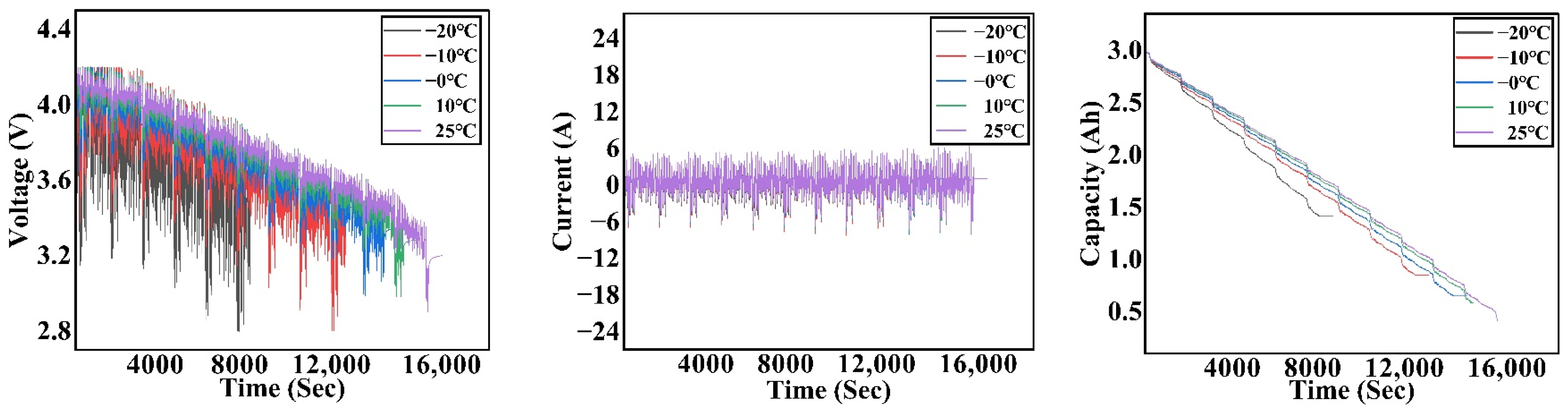
• Data from the LGHG2 18650 (H-NMC) lithium-ion cell under UDDS drive cycle conditions were used to evaluate model performance across a wide ambient temperature range (−20 °C to 25 °C).

1.4. Organization of This Article

This paper is organized as follows. After the introduction, Section 2 discusses the proposed framework for remaining capacity estimation using a GA. Section 3 provides details on data acquisition, experimental setup, and implementation details. Finally, Section 4 presents the results and discussion, while Section 5 concludes with a summary of the findings and future research directions.

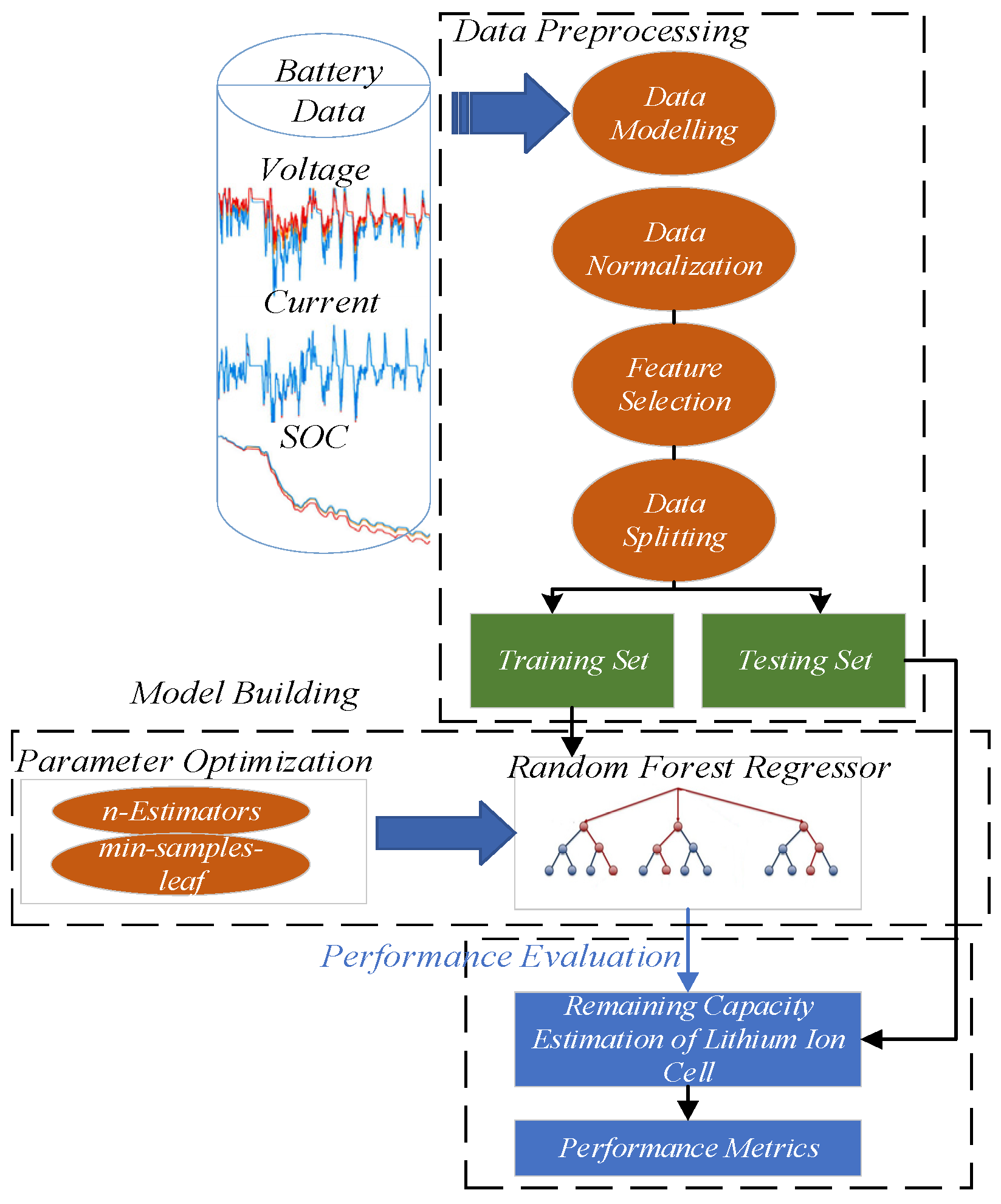
2. Proposed Framework for Remaining Capacity Estimation

The random forest regressor, a machine learning algorithm optimized using a GA, is utilized in this study to perform SOC estimation in lithium-ion batteries. The theory underlying this framework is presented in this section.

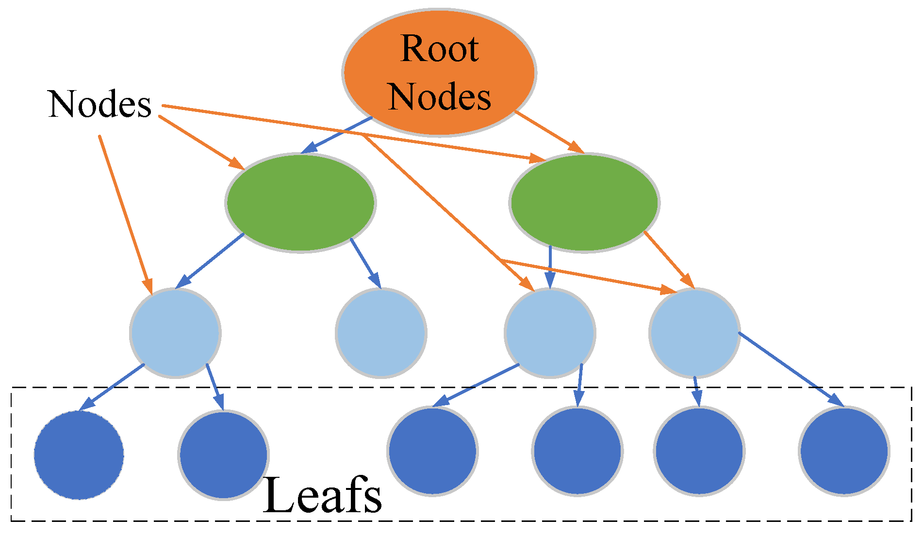
2.1. Random Forest Regressor for SOC Estimation

RF (Figure 1)is a general purpose machine learning technique that is frequently used for regression and classification applications. In this study, the remarkable regression capability of the RF model is utilized to precisely estimate the SOC of batteries used in electric vehicles. Leo Breiman first presented RF in 2001 [22]. An advanced form of the decision tree is the random forest [23]. A different subset of the training data is used to train each decision tree, and the outputs of all the trees are combined to get the final predictions. By training each decision tree on a random subset of the training data with replacement, RF uses the bagging method. This tactic improves model generalization and successfully lowers overfitting [24]. Due to its many benefits, RF is a good choice for the current SOC estimation assignment. It performs well with big, high-dimensional datasets, manages noisy data, and shows resilience to missing values and outliers. The number of trees in the forest is one of the key RF hyperparameters that greatly affect model performance. Hyperparameter adjustment was performed for the SOC estimation task to determine the optimal arrangement. The equations below form the core of RF regression and its training process.

(a)

Prediction Mechanism

$$\widehat{\mathrm{y}}={\displaystyle \frac{1}{\mathrm{N}}}\sum _{\mathrm{i}=1}^{\mathrm{N}}{\mathrm{T}}_{\mathrm{i}}\left(\mathrm{x}\right)$$

(2)

where $\widehat{\mathrm{y}}$ is the final predicted output, N is the total number of the decision tree, and Tx(x) is the prediction of the ith decision tree for input x.

(b)

Feature Importance

$${\mathrm{I}}_{\mathrm{f}}=\sum _{\mathrm{i}=1}^{\mathrm{N}}∆{\mathrm{G}}_{\mathrm{i}}\left(\mathrm{f}\right)$$

(3)

where $∆{\mathrm{G}}_{\mathrm{i}}\left(\mathrm{f}\right)$ is the improvement in the splitting criterion in tree i due to feature f.

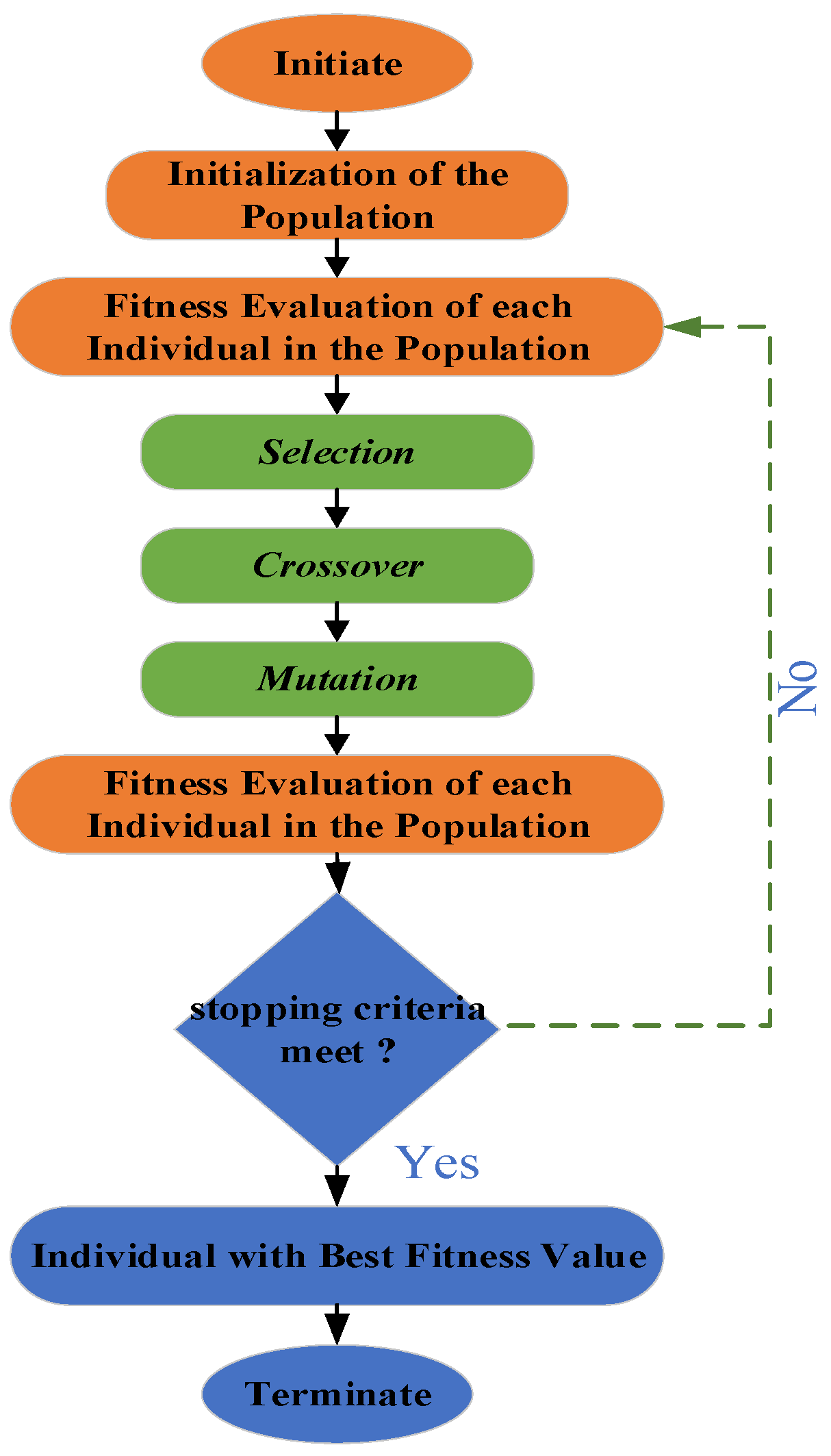
2.2. Genetic Algorithm for Parameter Optimization

Genetics and evolution provide the theoretical foundation for the GA, which scientist John Holland first created in 1975 [25]. The highly effective encoding method of the GA allows a solution vector to be represented as either a binary string or a real-coded string. Both encodings have different purposes in different problem domains. The GA is regarded as a global optimizer that can often identify a potential region, locate it, or even correctly obtain the optimum solution, which is also known as the global minimum [26,27]. The three operators that support this widely used method’s ability to function well in optimization jobs are as follows:

(i)

Selection: Using the idea of survival of the fittest, the goal is to provide preference to individuals (offspring) with high fitness scores and allow them to pass on their genes to future generations.

(ii)

Crossover: This denotes interindividual mating. The selection operator chooses a pair of individuals, and crossing sites are chosen at random. Subsequently, the genes at these crossover sites are transferred, creating an entirely new person. Throughout its duration, the crossover preserves and increases the diversity of the population.

(iii)

Mutation: The mutation operator inserts random genes into offspring to preserve population diversity by flipping certain chromosomal bits.

Below are set of equations related to the GA that are typically used for optimization problems.

(a)

Initialization of Population

P = {x₁, x₂…, x_n}

(4)

where P is the population of n individuals.

(b)

Selection

f(x_i) = Fitness (x_i)

(5)

where f(x_i) is the fitness of an individual x_i determined via a fitness evaluation function.

(c)

Crossover (Recombination)

P′ = Selection(P)

(6)

where P′ is the selected subset of the population based on fitness.

(d)

Crossover

Two parents x_i and x_j are selected, and crossover produces offspring x_new.

x_new = α·x_i + (1 − α) x_j

(7)

where α∈[0,1] is a random crossover parameter.

(e)

Mutation

x_i′ = x_i + δ

(8)

where δ is a small random perturbation.

(f)

Replacement

The new population P(t + 1) is formed by replacing some or all individuals from the previous generation.

P(t + 1) = Select from {x_new, xi}

(9)

(g)

Termination

The algorithm terminates when a stopping criterion is met, typically when the maximum number of generations G_max is reached or the solution converges.

Figure 2 illustrates the relevant figure that shows the GA workflow.

3. Data Acquisition, Experimental Setup, and Implementation Details

3.1. Data Collection and Cell Specifications

An LG 18650HG2 Li-ion battery with a nominal capacity of 3 Ah and a lithium nickel manganese cobalt oxide (LiNiMnCoO₂) chemistry was used to gather experimental datasets for SOC estimate. The cell has a long lifespan and a high specific energy. The LiNiMnCoO₂ cell’s key specifications are shown in

Table 2. Specifications of the Li-ion battery cell used in this study.

Specification	Details
Battery Model/Chemistry	LG HG2 18650 SN62A4/Lithium Nickel Manganese Cobalt Oxide (NMC)
Nominal Current/Open Circuit Voltage (OCV)	3 A/3.6 V
Nominal Capacity	3 Ah
Maximum Charge Voltage	4.2 V
Discharge Voltage (Cut-Off)	2.5 V (End of Discharge Cycle)
Charge/Discharge C-Rate	1.33 C (Charge)/6.67 C (Discharge)
Energy Density	240 Wh/kg

.

3.2. Drive Cycle and Testing Environment

An evaluation was conducted using a Li-ion LG 18650HG2 battery with a nominal capacity of 3 Ah to assess the effectiveness of the proposed RF-GA model. An open-source dataset, aggregated from the McMaster Automotive Resource Centre (MARC), was used for this purpose [28]. The power profiles tested included automotive industry-standard drive cycles, such as US06, LA92, UDDS, and HWFET, designed for electric vehicles. The battery was tested in a climate chamber with controlled conditions across six different temperatures: −20 °C, −10 °C, 0 °C, 10 °C, 25 °C, and 40 °C. Parameters such as temperature, voltage, current, and ampere hours were recorded. After each test, a 50 mA cut-off was applied, followed by 1C charging until the voltage reached 4.2 V. The battery was fully discharged before each new drive cycle, and recharging was performed using CC-CV (1C constant–current, constant–voltage) charging.

The model’s performance was evaluated using test data from the LA92 drive cycle conducted at six temperatures, −20 °C, −10 °C, 0 °C, 10 °C, and 25 °C, covering a broad spectrum of both low and moderate temperatures to ensure robustness across varying thermal conditions. Figure 3 presents the characteristic curves of the LG 18650HG2 Li-ion cell under UDDS cycle conditions.

3.3. Feature Selection for the Model

This paper presents a model for SOC estimation that leverages sensed data, such as battery terminal voltage (V), current (I), and cell temperature (T), along with newly developed features inspired by battery physics. Since feature selection plays a crucial role in data-driven approaches, this study also examines its influence on the SOC estimation accuracy of the proposed model. Different scenarios, each highlighting unique characteristics, are developed and analyzed individually, with the results compared to one another.

The battery voltage, current, temperature, average voltage, and average current are among the test inputs that are provided in the model. For the model input, three test cases with various combinations of these inputs were made.

(i)

Test Case I: In this scenario, the input features for the model consist of sensed battery data, including voltage (V), current (I), and temperature (T).

(ii)

Test Case II: In this scenario, the average battery voltage (V_avg) is included alongside voltage (V), current (I), and temperature (T). Incorporating V_avg provides valuable insights into the battery’s overall performance, and this feature is inspired by battery physics.

(iii)

Test Case III: In this scenario, historical voltage and current states are used as inputs, incorporating the mean values of the previous ‘N’ samples, V_avg, and average current (I_avg). These averages are calculated using a window size of 450 through a simple moving average technique, reflecting the battery’s dynamic transfer function and enhancing model learning for more accurate state estimation.

The average voltage and average current features were calculated using Python’s rolling average method with a window size of 450. This approach provides a smoothed representation of the data by averaging the values over the most recent 450 data points at any given time.

A window size of 450 was chosen based on empirical observation to balance between reducing noise and preserving important trends in the data. The rolling average was applied directly to the voltage and current data, without the need for a specific data sampling interval. Instead, it was designed to operate on sequential data points, where each window includes the most recent 450 measurements.

This method helped capture the battery’s dynamic behavior while reducing the impact of short-term fluctuations, improving the model’s ability to estimate SOC.

Table 3. Overview of test cases used for SOC estimation, detailing input features and configurations.

Cases	Test Inputs
Test Case I	Voltage (V), Current (I), Temperature (T)
Test Case II	Voltage (V), Current (I), Temperature (T), Average Voltage (Vavg)
Test Case III	Voltage (V), Current (I), Temperature (T), Average Voltage (Vavg), Average Current (Iavg)

illustrates the various battery features used for SOC estimation in the form of test cases.

3.4. Data Normalization

To account for differences in magnitude and units across battery parameters, such as voltage, current, and SOC, it is essential to standardize the data samples to improve the model’s training efficiency and performance. The min-max scaling function is applied to transform the measured values into the (0, 1) range, as demonstrated in Equation (10).

$${\mathrm{x}}^{*}={\displaystyle \frac{\mathrm{x}-{\mathrm{x}}_{\mathrm{m}\mathrm{i}\mathrm{n}}}{{\mathrm{x}}_{\mathrm{m}\mathrm{a}\mathrm{x}}-{\mathrm{x}}_{\mathrm{m}\mathrm{i}\mathrm{n}}}}$$

(10)

where x_min and x_max denote the minimum and maximum values observed in the real measurement data. x represents the actual measurement data, and x* signifies the normalized data.

3.5. Data Splitting

The data were divided into 70% for training and 30% for testing, ensuring that the model was trained on the majority of the data while still reserving a substantial portion for testing on unseen data. This split is standard practice to assess the model’s ability to generalize effectively. Although both training and testing were conducted under the same set of temperature conditions, the model is expected to generalize well to similar thermal environments. The use of RF, a robust machine learning technique, enables the model to capture the complex relationships between voltage, current, and temperature, ensuring reliable performance across a variety of operational conditions.

3.6. Implementation Details

This section outlines the implementation details of the experiments conducted to estimate the SOC of a Li-ion battery. The experiments are designed to evaluate the performance of an RF regressor model under different conditions, including the use of the GA for hyperparameter tuning and the variation of input features. Each set of experiments is described in detail below.

• In the first experiment, an RF regressor model estimates the SOC with three input features (voltage, current, temperature). Hyperparameters such as the number of estimators and minimum sample leaves are not tuned using the GA, and the minimum sample leaf value is kept fixed.
• In the second experiment, the GA is applied to optimize the hyperparameters of the RF model, specifically tuning the number of estimators and minimum sample split. The same input features are used, and the fixed minimum sample parameter ensures consistency. The hyperparameters that need to be optimized are listed in

  Table 4. List of hyperparameters selected for optimization in the SOC estimation model.

  RF Hyperparameters	Values (Fixed)	Value Range (Tuned with the GA)
  n_estimator	90	0–100
  min_samples_split	10	0–10
  min_samples_leaf	5	5 (Fixed)

  .
• In the third experiment, the RF regression model is applied with different sets of input features structured as test cases, without GA tuning. This experiment evaluates the impact of varying input features on SOC estimation accuracy.

The GA, inspired by natural selection, was used to optimize key hyperparameters of the RF model, including the number of estimators (n-estimators) and minimum samples per split (min-samples-split). The GA performs simultaneous optimization of all parameters by evaluating combinations of hyperparameters together in each generation, rather than tuning them independently. This allows the algorithm to account for the coupling of parameters, ensuring that the optimal combination is found by considering their interdependencies. The fitness of each combination is assessed based on the model’s performance in SOC estimation, and evolutionary operations, like crossover and mutation, are applied to explore new parameter configurations. The optimization ranges were chosen to be broad enough for the GA to explore a wide variety of configurations.

These ranges were selected to cover both lower values, where the model would have fewer decision trees and splits, and higher values, where the model would become more complex. This approach was intended to allow the GA to explore a variety of configurations and prevent the model from being either too simple (underfitting) or overly complex (overfitting). The specific range limits were selected randomly but with the intent to cover common values used in the literature and practice for similar models.

This paper utilizes a machine learning technique implemented through Scikit-learn [29], executed on a computer with a Core i7 3.60 GHz processor and 32 GB of RAM, Intel 2017, Santa Clara, CA, USA. Figure 4 illustrates the workflow of the proposed model.

3.7. Performance Metrics

To assess the effectiveness of the RF-GA model, various metrics were utilized, including the MAE, RMSE, and Maximum Error (MAX ERROR). The definitions of these metrics are as follows:

$$\mathrm{M}\mathrm{A}\mathrm{E}={\displaystyle \frac{1}{\mathrm{N}}}\sum _{\mathrm{i}=1}^{\mathrm{N}}\left({\left({\mathrm{x}}_{\mathrm{m}\mathrm{e}\mathrm{a}\mathrm{s}\mathrm{u}\mathrm{r}\mathrm{e}\mathrm{d}}\right)}_{\mathrm{i}}-{\left({\mathrm{x}}_{\mathrm{p}\mathrm{r}\mathrm{e}\mathrm{d}\mathrm{i}\mathrm{c}\mathrm{t}\mathrm{e}\mathrm{d}}\right)}_{\mathrm{i}}\right)$$

(11)

$$\mathrm{R}\mathrm{M}\mathrm{S}\mathrm{E}=\sqrt{\sum _{\mathrm{i}=1}^{\mathrm{N}}{\left({\displaystyle \frac{{\left({\mathrm{x}}_{\mathrm{m}\mathrm{e}\mathrm{a}\mathrm{s}\mathrm{u}\mathrm{r}\mathrm{e}\mathrm{d}}\right)}_{\mathrm{i}}-{\left({\mathrm{x}}_{\mathrm{p}\mathrm{r}\mathrm{e}\mathrm{d}\mathrm{i}\mathrm{c}\mathrm{t}\mathrm{e}\mathrm{d}}\right)}_{\mathrm{i}}}{\mathrm{N}}}\right)}^2}$$

(12)

$$\mathrm{M}\mathrm{A}\mathrm{X}=\mathrm{m}\mathrm{a}\mathrm{x}\left({({\mathrm{x}}_{\mathrm{m}\mathrm{e}\mathrm{a}\mathrm{s}\mathrm{u}\mathrm{r}\mathrm{e}\mathrm{d}})}_{\mathrm{i}}-{({\mathrm{x}}_{\mathrm{p}\mathrm{r}\mathrm{e}\mathrm{d}\mathrm{i}\mathrm{c}\mathrm{t}\mathrm{e}\mathrm{d}})}_{\mathrm{i}}\right)$$

(13)

where $\mathrm{x}$ is the output values of the model.

4. SOC Estimation Results and Discussions

The following section consists of the results of the various experiments described in the previous section.

In this study, separate RF models were trained for each temperature condition, specifically for −10 °C, −20 °C, 0 °C, and 25 °C, using the UDDS load profile. This approach was chosen to reduce the computational burden on the system, as training a single model for all temperature conditions would have required significantly more resources and potentially impacted performance.

Each RF model was individually optimized using a GA to fine tune the hyperparameters, such as the number of estimators and the minimum number of samples per split. By tailoring the model for each specific temperature, we ensured that the SOC estimation was as accurate as possible under each thermal condition. The GA was employed to optimize key hyperparameters, such as the following:

• Number of Estimators (n_estimators): The number of decision trees in the forest.
• Minimum Samples per Split (min_samples_split): The minimum number of samples required to split an internal node.

The decision to train separate models for each temperature allowed for better handling of the unique thermal effects on battery performance. Different temperatures impact the electrochemical processes inside the battery, leading to variations in its dynamic behavior. By creating a dedicated model for each thermal condition, we minimized the need for the model to generalize across a wide range of temperatures, improving accuracy and reducing computational complexity.

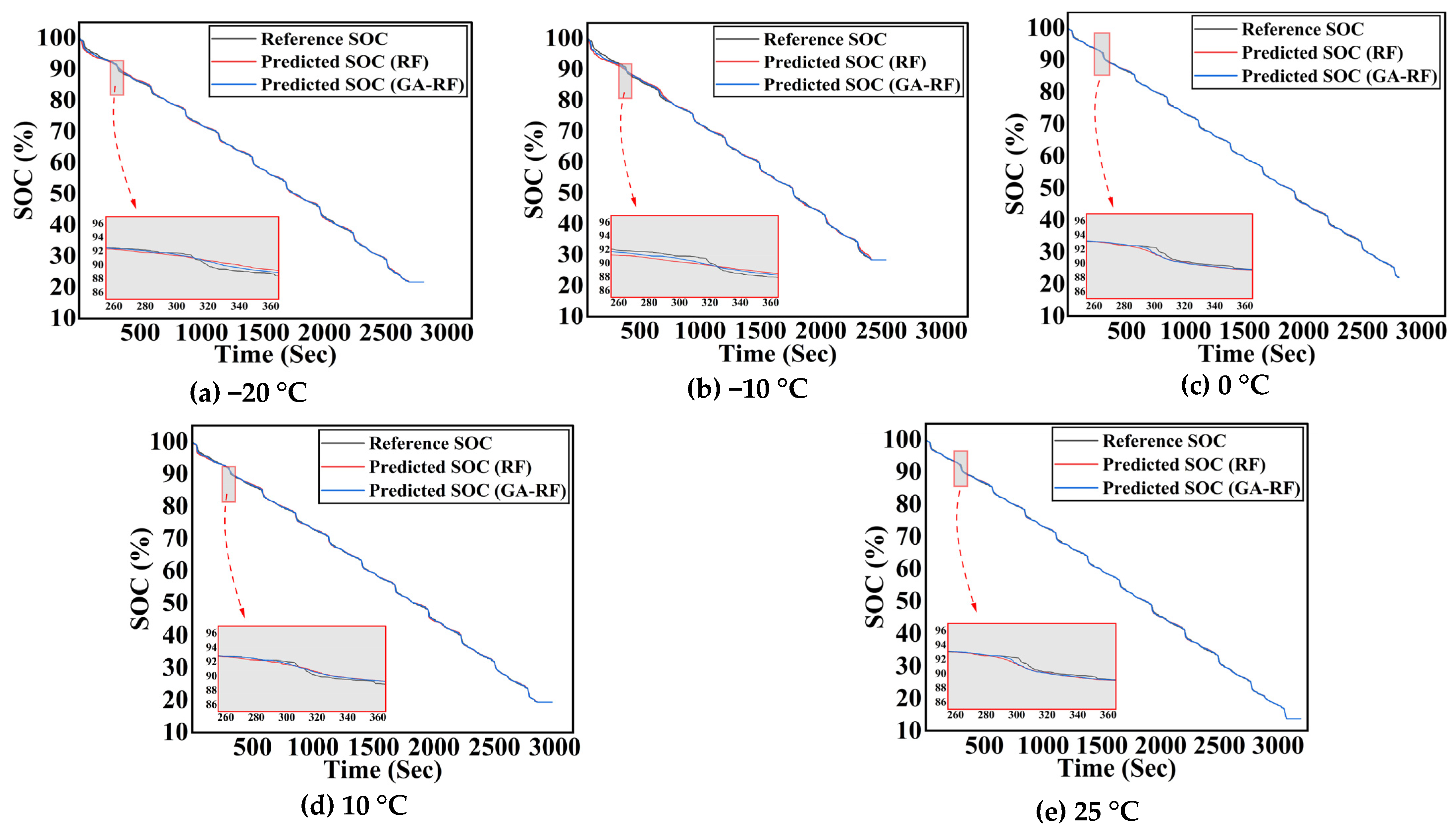
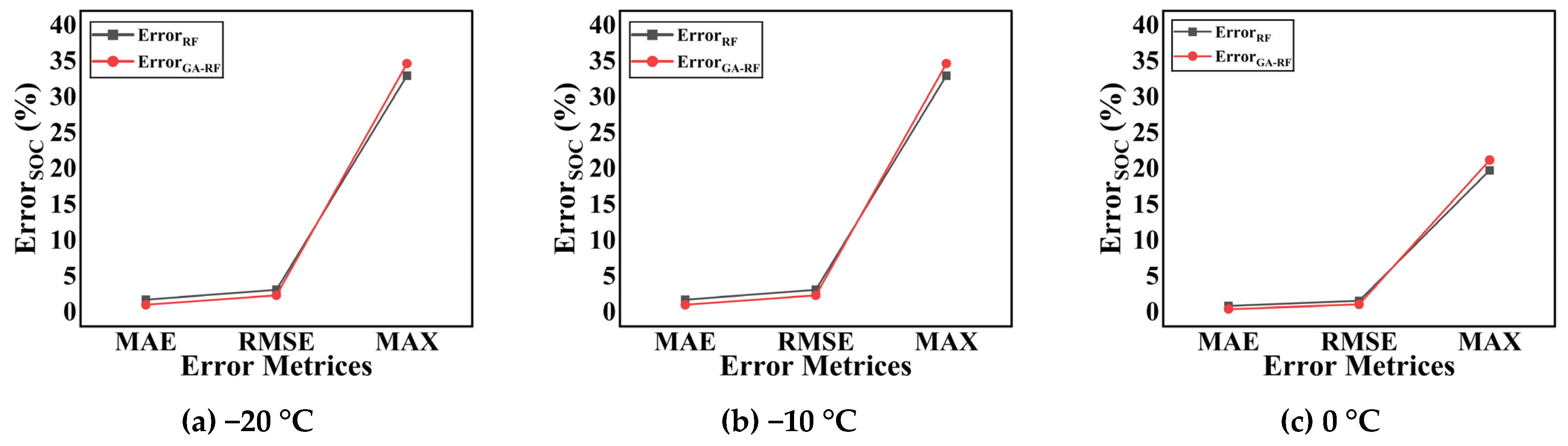
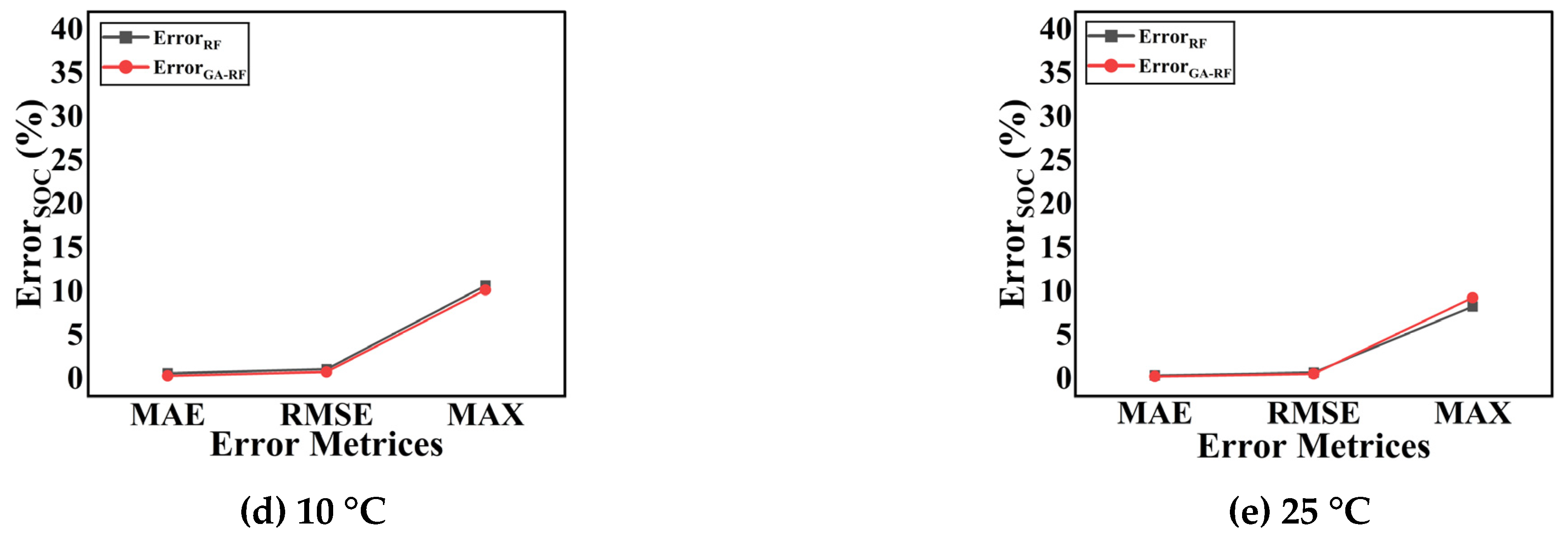
4.1. SOC Estimation Results Using an RF Regressor and a GA-Tuned RF Regressor Under Varying Ambient Thermal Conditions

In this section, the proposed GA-RF model is compared with the RF. In this experiment, the proposed GA-RF model is compared with the basic RF model without tuning implemented in this work. The experiments are performed at temperatures of −20 °C, −10 °C, 0 °C, 10 °C, and 25 °C. The drive cycle used for the experimentation of both the RF and GA-RF is the UDDS, known as a dynamic drive cycle.

Table 5. Estimation errors of random forest (RF) and GA-optimized random forest (GA-RF) at various temperatures.

Temperature (°C)/Error Metrics	MAE (%) (RF/GA-RF)	RMSE (%) (RF/GA-RF)	MAX (%) (RF/GA-RF)
−20	0.0174/0.0102	0.0313/0.0235	0.3297/0.3467
−10	0.0121/0.0065	0.0227/0.0161	0.2264/0.2247
0	0.0086/0.0043	0.0158/0.0109	0.1976/0.2121
10	0.0061/0.0033	0.0110/0.0078	0.1067/0.1018
25	0.0038/0.0026	0.0070/0.0057	0.0827/0.0928

shows the SOC-estimated results of both the RF and GA-RF models. As the temperature increases, the estimation results improve, and the GA-RF model shows improved results compared to the traditional RF model. The MAE and RMSE of the GA-RF improved compared to the RF algorithm by 41.37% and 24.92%, respectively, at −20 °C, 46.28% and 29.07%, respectively, at −10 °C, 50% and 31.01%, respectively, at 0 °C, 45.90% and 29.09% at 10 °C, and 31.87% and 18.57%, respectively, at 25 °C. Whereas the MAX error improves for −10 °C and 10 °C by 0.75% and 4.95%, respectively the MAX error increases for temperatures other than −10 °C and 10 °C.

The following conclusions can be drawn from the tables discussed above and the comparison plot shown below:

• By applying the GA, these hyperparameters are systematically optimized through an evolutionary process that searches for the best possible combination. The GA iterates over generations, selecting hyperparameter sets based on fitness criteria (e.g., minimizing SOC estimation MAE), applying crossover and mutation to explore the search space, and eventually converging on the optimal values. This optimization improves the model’s ability to capture patterns in the input data (voltage, current, temperature) more effectively, leading to enhanced prediction accuracy and a significant reduction in the SOC estimation MAE.
• The SOC estimation MAE tends to decrease as the temperature of the battery cell increases because the electrochemical reactions within the cell become more consistent and stable at higher temperatures. This stability reduces fluctuations in voltage and current readings, allowing the model to estimate the SOC more accurately.

The estimation results are illustrated in Figure 5, which shows the SOC curve of reference SOC, estimated SOC by RF, and estimated SOC by the GA-SOC algorithm; also, the error results are graphically represented in Figure 6.

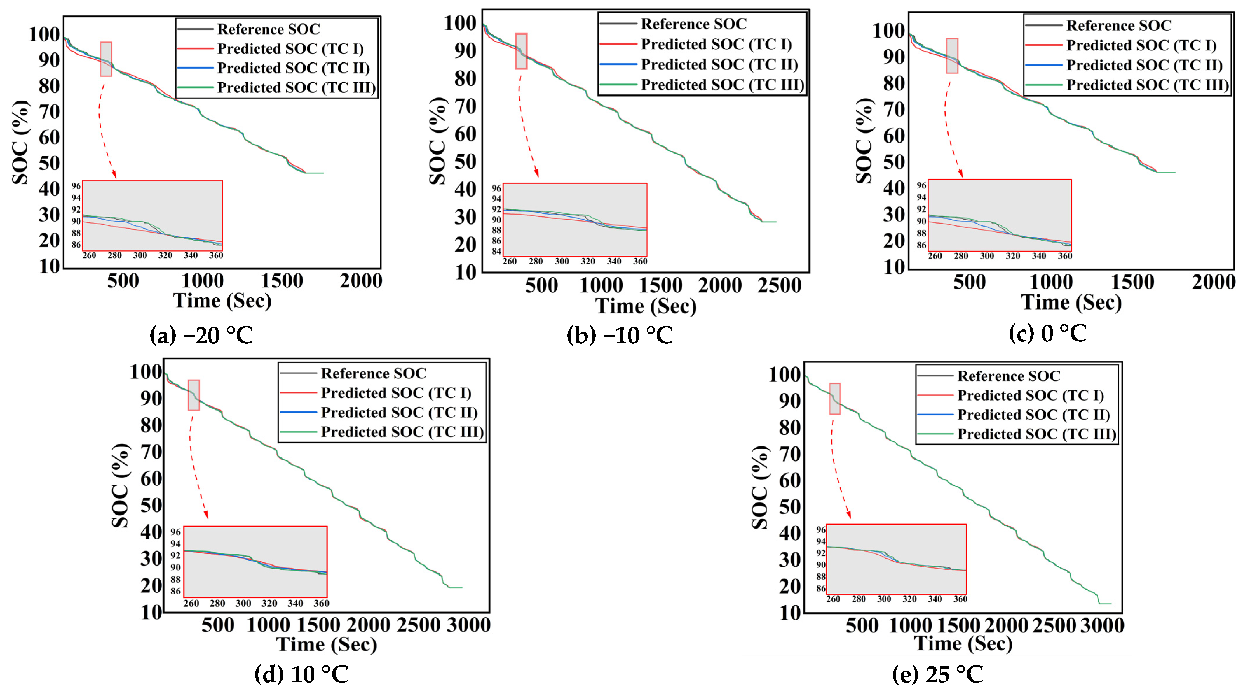
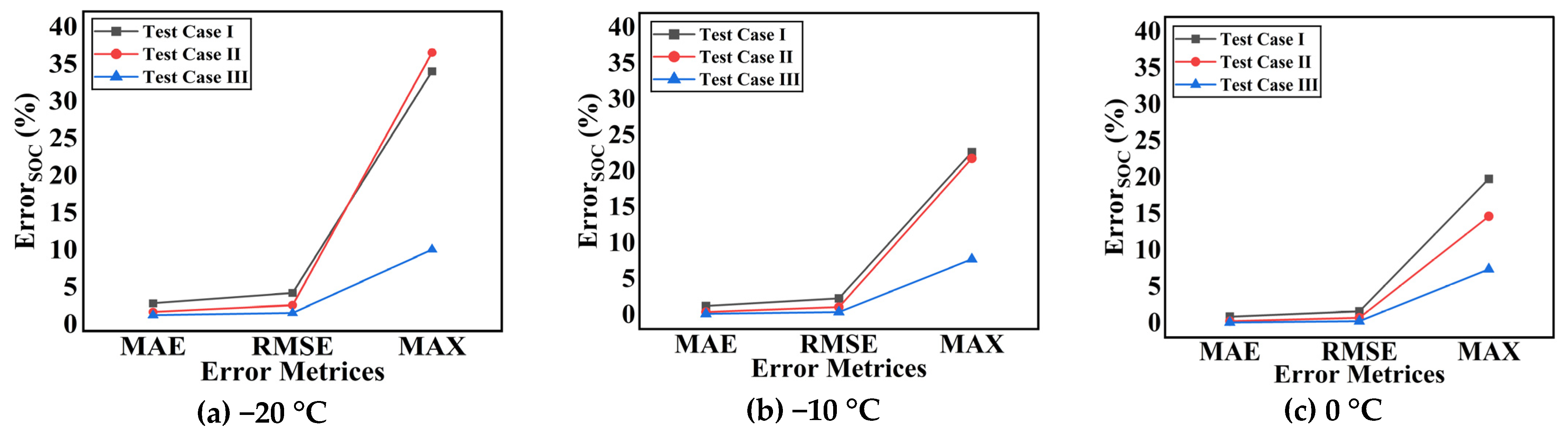
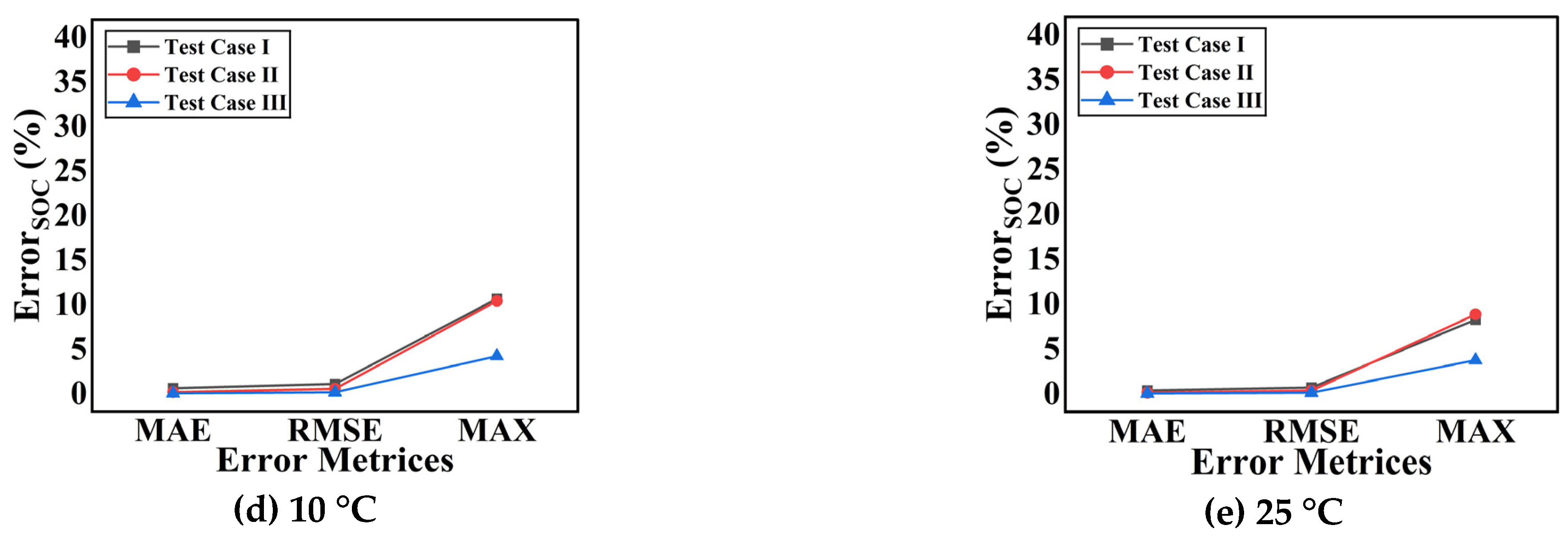
4.2. SOC Estimation Results Using the RF Regressor Under Varying Input Features

The three test cases are developed using the different combinations of inputs; the test case combination is illustrated in Table 3. The data from McMaster University is used in this experimentation, which comprise the dataset at temperatures −20 °C, −10 °C, 0 °C, 10 °C, and 25 °C. The battery voltage and current are used to create the additional inputs, i.e., average voltage and average current. By incorporating these inputs in the training phase, the estimation results improved.

Table 6. Performance metrics of SOC estimation for the RF regressor under varying ambient temperatures at varying input feature conditions.

Temperature (°C)/Error Metrics	MAE (%) Test Case (I/II/III)	RMSE (%) Test Case (I/II/III)	MAX (%) Test Case (I/II/III)
−20	1.74/0.57/0.13	3.13/1.48/0.42	32.97/35.48/08.97
−10	1.21/0.37/0.10	2.27/1.05/0.35	22.64/21.76/7.73
0	0.86/0.24/0.07	1.58/0.71/0.24	19.76/14.63/7.37
10	0.61/0.19/0.05	1.10/0.56/0.17	10.67/10.43/4.24
25	0.38/0.13/0.04	0.70/0.37/0.13	8.27/8.87/3.77

shows the SOC estimation results of three test cases at five different temperatures that were specified earlier.

It can be seen from the results that test case II is better than test case I, whereas test case III shows far better results than test case II and test case I. The incorporation of additional inputs to the training phase of the RF model improved the results and also made it easy to implement. Test case III shows a decrease in the MAE by 67.24% compared to test case I and 77.19% compared to test case II, and the RMSE decreased by 86.58% compared to test case I and 71.62% compared to test case II at −20 °C. For −10 °C, the MAE decreased by 91.73% compared to test case I and 72.97% compared to test case II, and the RMSE decreased by 84.58% compared to test case I and 66.67% compared to test case II. For 0 °C, the MAE decreased by 91.86% compared to test case I and 70.83% compared to test case II, and the RMSE decreased by 84.81% compared to test case I and 66.19% compared to test case II. For 10 °C, the MAE decreased by 91.80% compared to test case I and 73.68% compared to test case II, and the RMSE decreased by 84.54% compared to test case I and 69.64% compared to test case II. For 25 °C, the MAE decreased by 89.47% compared to test case I and 69.25% compared to test case II, and the RMSE decreased by 81.42% compared to test case I and 64.86% compared to test case II.

The following inferences can be made from the tables discussed above and the comparison plot shown below:

• While voltage and temperature are traditionally considered crucial for SOC estimation, the inclusion of the current and its rolling average is equally important. The current directly impacts the rate of charge and discharge, making it a fundamental factor in SOC estimation. By incorporating the rolling averages of both voltage and current, short-term spikes and fluctuations are mitigated, thereby improving the model’s stability and accuracy.
• As the number of input attributes increases in the RF model, the MAE decreases because the model can better capture patterns and relationships. More inputs offer the model a longer sequence to analyze, improving its ability to recognize long-term patterns. Additionally, with more attributes, the model becomes more adaptable to a wider range of conditions, leading to more accurate predictions, even in the presence of variations or unforeseen scenarios.
• Introducing previous samples of V and I significantly reduces MAE, RMSE, and MAX values because it allows the model to capture temporal dependencies and dynamic behavior of the battery. By including historical data, the model can better understand trends and patterns over time, such as the battery’s response to varying loads and conditions. This additional temporal context enhances the model’s predictive accuracy by smoothing out fluctuations and improving its ability to predict future states based on past behavior, leading to a more accurate and reliable SOC estimation.

As shown in Table 6, comparative experiments demonstrate that including the rolling averages of both current and voltage, along with other features, significantly enhances SOC estimation accuracy. The rolling averages provide a smoother, more consistent input to the model, which better represents the battery’s overall behavior under dynamic conditions like those seen in the UDDS cycle.

To evaluate the effectiveness of the proposed RF model, we conducted a comparative analysis against other widely used SOC estimation models. The key performance metric considered in this comparison is the MAE, which reflects the accuracy of the SOC estimation under various temperature conditions.

Table 7. SOC estimation performance comparison across different temperatures and test cases along with a comparative analysis against other widely used SOC estimation models.

Temperature (°C)	Model	MAE (%)		Drive Cycle	Reference
–20	Traditional RF Model	Test Case I	1.74	UDDS	This Study
		Test Case II	0.57
		Test Case III	0.13
–20	PSO-LSTM [Ren et al., 2021]	0.4307		New European Drive Cycle (NEDC)	[17]
–10	Traditional RF Model	Test Case I	1.21	UDDS	This Study
		Test Case II	0.37
		Test Case III	0.10
0	Traditional RF Model	Test Case I	0.86	UDDS	This Study
		Test Case II	0.24
		Test Case III	0.07
0	Bayesian BiLSTM [Yang et al., 2022]	0.93		BJDST, US06, DST, FUDS	[16]
0	LSTM-UKF [Zhang et al., 2021]	0.63		US06, DST, FUDS	[15]
0	The Fb-Ada-CNNGRU-KF	0.13/0.39		HWFET/UDDS	[20]
10	Traditional RF Model	Test Case I	0.61	UDDS	This Study
		Test Case II	0.19
		Test Case III	0.05
10	LSTM-UKF [Zhang et al., 2021]	0.21		US06, DST, FUDS	[15]
10	The Fb-Ada-CNNGRU-KF	0.16/0.54		HWFET/UDDS	[20]
25	Traditional RF Model	Test Case I	0.38	UDDS	This Study
		Test Case II	0.13
		Test Case III	0.04
25	The Fb-Ada-CNNGRU-KF	0.18/0.70		HWFET/UDDS	[20]

below presents the results, showing the effectiveness of the RF model, particularly in terms of the MAE, where it demonstrates a significant improvement over traditional RF models and other machine learning-based approaches.

Figure 7 illustrates SOC estimation under varying input feature conditions. Additionally, the error results for this experiment are graphically represented in Figure 8.

When comparing the results of this paper with previous studies [13,14,16,17,18,19] presented in Table 1, a clear trend emerges, demonstrating enhanced accuracy and reliability in SOC estimation using the RF-GA approach. The findings consistently indicate that this method represents a significant advancement over prior work, highlighting the effectiveness and robustness of the proposed random forest model optimized by a Genetic Algorithm in addressing the complexities of SOC estimation in lithium-ion batteries. This underscores the strength and efficacy of the RF-GA method for estimating the SOC in lithium-ion batteries.

5. Conclusions

This paper presented an RF model optimized by the GA for SOC estimation of lithium-ion batteries. The proposed approach effectively addresses the complexities associated with SOC estimation, demonstrating enhanced accuracy and reliability compared to previous methodologies. By incorporating various input features and utilizing historical voltage and current data, our model significantly reduces error metrics such as the MAE, RMSE, and MAX error. The results validate the robustness of the RF-GA model in adapting to diverse operational conditions, making it a strong candidate for practical applications in battery management systems. Despite the promising outcomes of our study, there are some limitations of the current approach, which include substantial computational resources, particularly during the hyperparameter tuning process, which could hinder its deployment in resource-constrained environments. As new battery technologies emerge, the model may need retraining or adjustments to maintain its effectiveness, highlighting the need for ongoing research in this area. Future studies should prioritize the development of a real-time version of the RF-GA model to enable its application in practical scenarios, allowing for continuous SOC estimation during battery operation. Additionally, expanding the dataset to include a broader range of operating conditions and various battery types would enhance the model’s generalizability. Furthermore, integrating the RF-GA model with other machine learning techniques, such as deep learning or ensemble methods, could significantly improve estimation accuracy and reliability.

References

1. International Energy Agency Report Predicts 2024 EV Sales Surge. Available online: https://electricautonomy.ca/automakers/2024-05-17/report-ev-sales-iea-global-ev-outlook/ (accessed on 18 September 2024).
2. Beaudet, A.; Larouche, F.; Amouzegar, K.; Bouchard, P.; Zaghib, K. Key Challenges and Opportunities for Recycling Electric Vehicle Battery Materials. Sustainability 2020, 12, 5837. [Google Scholar] [CrossRef]
3. Sanguesa, J.A.; Torres-Sanz, V.; Garrido, P.; Martinez, F.J.; Marquez-Barja, J.M. A Review on Electric Vehicles: Technologies and Challenges. Smart Cities 2021, 4, 372–404. [Google Scholar] [CrossRef]
4. Riggs, H.; Tufail, S.; Parvez, I.; Tariq, M.; Khan, M.A.; Amir, A.; Vuda, K.V.; Sarwat, A.I. Impact, Vulnerabilities, and Mitigation Strategies for Cyber-Secure Critical Infrastructure. Sensors 2023, 23, 4060. [Google Scholar] [CrossRef] [PubMed]
5. Stevenson, A.; Tariq, M.; Sarwat, A. Reduced Operational Inhomogeneities in a Reconfigurable Parallelly-Connected Battery Pack Using DQN Reinforcement Learning Technique. In Proceedings of the 2023 IEEE Transportation Electrification Conference & Expo (ITEC), Chiang Mai, Thailand, 28 November–1 December 2023; IEEE: Piscataway, NJ, USA, 2023; pp. 1–5. [Google Scholar]
6. Liu, F.; Liu, T.; Fu, Y. An Improved SoC Estimation Algorithm Based on Artificial Neural Network. In Proceedings of the 2015 8th International Symposium on Computational Intelligence and Design (ISCID), Hangzhou, China, 12–13 December 2015; Volume 2, pp. 152–155. [Google Scholar] [CrossRef]
7. Khan, U.; Kirmani, S.; Rafat, Y.; Rehman, M.U.; Alam, M.S. Improved Deep Learning Based State of Charge Estimation of Lithium Ion Battery for Electrified Transportation. J. Energy Storage 2024, 91, 111877. [Google Scholar] [CrossRef]
8. Chandran, V.; Patil, C.K.; Karthick, A.; Ganeshaperumal, D.; Rahim, R.; Ghosh, A. State of Charge Estimation of Lithium-Ion Battery for Electric Vehicles Using Machine Learning Algorithms. World Electr. Veh. J. 2021, 12, 38. [Google Scholar] [CrossRef]
9. Chemali, E.; Kollmeyer, P.J.; Preindl, M.; Ahmed, R.; Emadi, A. Long Short-Term Memory Networks for Accurate State-of-Charge Estimation of Li-Ion Batteries. IEEE Trans. Ind. Electron. 2018, 65, 6730–6739. [Google Scholar] [CrossRef]
10. Hossain Lipu, M.S.; Hannan, M.A.; Hussain, A.; Ayob, A.; Saad, M.H.M.; Muttaqi, K.M. State of Charge Estimation in Lithium-Ion Batteries: A Neural Network Optimization Approach. Electronics 2020, 9, 1546. [Google Scholar] [CrossRef]
11. How, D.N.T.; Hannan, M.A.; Hossain Lipu, M.S.; Ker, P.J. State of Charge Estimation for Lithium-Ion Batteries Using Model-Based and Data-Driven Methods: A Review. IEEE Access 2019, 7, 136116–136136. [Google Scholar] [CrossRef]
12. de Lima, A.B.; Salles, M.B.C.; Cardoso, J.R. State-of-Charge Estimation of a Li-Ion Battery Using Deep Forward Neural Networks. arXiv 2020, arXiv:2009.09543. [Google Scholar]
13. Tian, J.; Chen, C.; Shen, W.; Sun, F.; Xiong, R. Deep Learning Framework for Lithium-Ion Battery State of Charge Estimation: Recent Advances and Future Perspectives. Energy Storage Mater. 2023, 61, 102883. [Google Scholar] [CrossRef]
14. Hannan, M.A.; Lipu, M.S.H.; Hussain, A.; Ker, P.J.; Mahlia, T.M.I.; Mansor, M.; Ayob, A.; Saad, M.H.; Dong, Z.Y. Toward Enhanced State of Charge Estimation of Lithium-Ion Batteries Using Optimized Machine Learning Techniques. Sci. Rep. 2020, 10, 4687. [Google Scholar] [CrossRef] [PubMed]
15. Yang, F.; Zhang, S.; Li, W.; Miao, Q. State-of-Charge Estimation of Lithium-Ion Batteries Using LSTM and UKF. Energy 2020, 201, 117664. [Google Scholar] [CrossRef]
16. Yang, B.; Wang, Y.; Zhan, Y. Lithium Battery State-of-Charge Estimation Based on a Bayesian Optimization Bidirectional Long Short-Term Memory Neural Network. Energies 2022, 15, 4670. [Google Scholar] [CrossRef]
17. Ren, X.; Liu, S.; Yu, X.; Dong, X. A Method for State-of-Charge Estimation of Lithium-Ion Batteries Based on PSO-LSTM. Energy 2021, 234, 121236. [Google Scholar] [CrossRef]
18. Eleftheriadis, P.; Leva, S.; Ogliari, E. Bayesian Hyperparameter Optimization of Stacked Bidirectional Long Short-Term Memory Neural Network for the State of Charge Estimation. Sustain. Energy Grids Netw. 2023, 36, 101160. [Google Scholar] [CrossRef]
19. El Fallah, S.; Kharbach, J.; Hammouch, Z.; Rezzouk, A.; Ouazzani Jamil, M. State of Charge Estimation of an Electric Vehicle’s Battery Using Deep Neural Networks: Simulation and Experimental Results. J. Energy Storage 2023, 62, 106904. [Google Scholar] [CrossRef]
20. Yang, Y.; Zhao, L.; Yu, Q.; Liu, S.; Zhou, G.; Shen, W. State of Charge Estimation for Lithium-Ion Batteries Based on Cross-Domain Transfer Learning with Feedback Mechanism. J. Energy Storage 2023, 70, 108037. [Google Scholar] [CrossRef]
21. Sulaiman, M.H.; Mustaffa, Z. State of Charge Estimation for Electric Vehicles Using Random Forest. Green Energy Intell. Transp. 2024, 3, 100177. [Google Scholar] [CrossRef]
22. Breiman, L. Random Forests. Mach. Learn. 2001, 45, 5–32. [Google Scholar] [CrossRef]
23. Tufail, S.; Riggs, H.; Tariq, M.; Sarwat, A.I. Advancements and Challenges in Machine Learning: A Comprehensive Review of Models, Libraries, Applications, and Algorithms. Electronics 2023, 12, 1789. [Google Scholar] [CrossRef]
24. Probst, P.; Wright, M.N.; Boulesteix, A. Hyperparameters and Tuning Strategies for Random Forest. WIREs Data Min. Knowl. Discov. 2019, 9, e1301. [Google Scholar] [CrossRef]
25. Sivanandam, S.N.; Deepa, S.N. Genetic Algorithms. In Introduction to Genetic Algorithms; Springer: Berlin/Heidelberg, Germany, 2008; pp. 15–37. [Google Scholar]
26. Lee, J.B.; Lee, B.C. A global optimization algorithm based on the new filled function method and the genetic algorithm. Eng. Optim. 1996, 27, 1–20. [Google Scholar] [CrossRef]
27. Ting, T.O.; Man, K.L.; Lim, E.G.; Leach, M. Tuning of Kalman Filter Parameters via Genetic Algorithm for State-of-Charge Estimation in Battery Management System. Sci. World J. 2014, 2014, 1–11. [Google Scholar] [CrossRef]
28. Kollmeyer, P.; Vidal, C.; Naguib, M.; Skells, M. LG 18650HG2 Li-Ion Battery Data and Example Deep Neural Network XEV SOC Estimator Script. Mendeley Data 2020. [Google Scholar] [CrossRef]
29. RandomForestClassifier—Scikit-Learn 1.5.2 Documentation. Available online: https://scikit-learn.org/stable/modules/generated/sklearn.ensemble.RandomForestClassifier.html (accessed on 28 September 2024).
Figure 1. Diagram illustrating the random forest regression process.
Energies 17 05582 g001
Figure 2. Genetic Algorithm process for optimizing.
Energies 17 05582 g002
Figure 3. UDDS drive cycle characteristics under different temperature conditions.
Energies 17 05582 g003
Figure 4. Workflow of the proposed model for SOC estimation using GA-tuned random forest regression.
Energies 17 05582 g004
Figure 5. SOC estimation curve comparing reference SOC and estimated SOC values under varying ambient temperatures.
Energies 17 05582 g005
Figure 6. Graphical representation of error results for SOC estimation under varying ambient temperatures.
Energies 17 05582 g006aEnergies 17 05582 g006b
Figure 7. SOC estimation curve comparing reference SOC and estimated SOC values under varying ambient temperatures at varying input feature conditions.
Energies 17 05582 g007
Figure 8. Graphical representation of error results for SOC estimation under varying ambient temperatures and varying input feature conditions.
Energies 17 05582 g008aEnergies 17 05582 g008b