Remaining Service Life Prediction of Lithium-Ion Batteries Based on Randomly Perturbed Traceless Particle Filtering

Abstract

To address the limitations in the prediction accuracy of the remaining useful life (RUL) of lithium-ion batteries, stemming from model accuracy, particle degradation, and insufficient diversity in the particle filter (PF) algorithm, this paper proposes a battery RUL prediction method utilizing a randomly perturbed unscented particle filter (RP-UPF) algorithm, based on the constructed battery capacity degradation model. The method utilizes evaluation metrics adjusted R-squared (R_adj²) and the Akaike Information Criterion (AIC) to select the battery capacity decline model C₅ with a higher goodness of fit. The initial values for constructing the C₅ model are obtained using the relevance vector machine (RVM) and nonlinear least squares methods. Based on the constructed battery capacity decline model C₅, the RP-UPF algorithm is employed to estimate the posterior parameters and iteratively approach the true battery capacity decline curve, thereby predicting the battery’s RUL. The research results indicate that, using battery B0005 as an example and starting the prediction from the 50th cycle, the RUL prediction results obtained with the RP-UPF algorithm demonstrate reductions in absolute error, relative error, and probability density function (PDF) width of 2%, 2.71%, and 10%, respectively, compared to the PF algorithm. Similar conclusions were drawn for batteries B0006 and B0018. Under the constructed battery capacity degradation model C₅, the RP-UPF algorithm shows higher prediction accuracy for battery RUL and a narrower PDF range compared to the PF algorithm. This approach effectively addresses the issue of particle weight degradation in the PF algorithm, providing a more valuable reference for battery RUL prediction.

1. Introduction

As the automotive industry rapidly advances, issues such as environmental pollution, global warming, and rising energy consumption are becoming increasingly severe, making the development of electric vehicles a major trend [1]. Traction batteries, as core components of electric vehicles, directly impact their range, acceleration performance, safety, and lifespan [2]. However, batteries inevitably undergo aging and even failure during long-term cyclic use. Therefore, accurately predicting the RUL of batteries has become a focal point in battery research.

Currently, three main methods are commonly used for predicting the RUL of lithium-ion batteries: model-based prediction, data-driven prediction, and fusion-based prediction [3].

The model-based prediction method involves establishing aging models based on the internal electrochemical characteristics and performance degradation mechanisms of batteries, which reflect the operational patterns of batteries and predict their RUL [4]. For example, Lyu et al. [5] analyzed the internal operation mechanisms of batteries based on electrochemical models. They utilized the principles of battery electrochemical reactions combined with PF methods to establish models of battery capacity degradation mechanisms for predicting the RUL of batteries. Miao et al. [6] predicted the RUL of batteries using an empirical capacity fade model and UPF algorithm. Guha et al. [7] proposed a fractional-order equivalent circuit model capable of online estimation of battery internal resistance. This model employs recursive least squares techniques and fractional-order variable filters to determine the model parameters, allowing the estimation of electrochemical impedance under various aging conditions for predicting battery RUL. Although model-based RUL prediction methods have achieved success, establishing precise physical degradation models for battery systems remains challenging in practical applications. In contrast, empirical degradation models are more accessible and require less effort than mechanistic degradation models and equivalent circuit models, leading to their widespread use. Additionally, filtering algorithms, which do not require extensive data, can utilize the dynamic equations of the battery system as degradation observation equations, playing a crucial role in the research on battery life prediction.

The data-driven prediction method involves establishing predictive models based on the dynamic changes in external battery data and the patterns of battery performance degradation, without considering the internal battery mechanisms. For example, Zhou et al. [8] proposed a battery RUL prediction method based on an expanded convolutional neural network. Wang et al. [9] introduced a battery RUL prediction model combining convolutional neural networks with long short-term memory networks. Ansari et al. [10] proposed a cascaded feedforward neural network for battery RUL prediction under various input profiles. Similarly, Patil et al. [11] introduced a multi-model fusion support vector machine (SVM) method that meets the accuracy requirements for battery RUL prediction under different operating conditions. Compared to model-based RUL prediction methods, data-driven approaches do not require consideration of the complex physical and chemical processes occurring within the battery, making them more versatile. However, precise predictions using data-driven methods necessitate a substantial amount of historical data; otherwise, the accuracy of the predictions may be compromised. Therefore, reducing reliance on historical data while improving computational efficiency has become a focal point of research in data-driven battery RUL prediction.

Some scholars have also adopted data-driven and fusion-based methods for predicting battery RUL. For instance, Zeng et al. [12] proposed a fusion approach combining model-based and data-driven methods to forecast battery RUL. Their study involved establishing an error compensation model using data-driven methods to supplement degradation information in empirical capacity fade models of batteries. Liu et al. [13] utilized an autoregressive time series model as the observation equation and employed the PF algorithm to achieve battery RUL prediction. Dolenc et al. [14] employed a fusion method that combined Kalman filtering (KF) and particle swarm optimization for battery RUL prediction. Chen et al. [15] proposed a battery RUL prediction method that integrates a linear optimization resampling particle filter with a sliding window gray model. While fusion methods can leverage the strengths of different prediction approaches for battery RUL estimation, the selection, combination, and parameter tuning of various methods can be more complex. This complexity can lead to issues such as computational intensity, large operational loads, and uncertainties in the fusion process [16].

Based on the above analysis, to address the challenges associated with establishing accurate physical degradation models for battery systems in existing model-based prediction methods, this study focuses on lithium-ion batteries. Utilizing model-based prediction methods, the study builds a battery capacity degradation model with a simpler structure and better fit, based on the analysis of empirical models of battery capacity decline. Subsequently, the study employs the RP-UPF algorithm for lithium-ion battery RUL prediction. The RP-UPF algorithm initializes the state through sampling from a prior distribution to be more direct. During the importance sampling phase, it uses the Unscented Kalman Filter (UKF) to calculate the mean and variance, normalizes the particle weights using the latest observations, and updates the particle weights through random perturbation resampling. This approach addresses the issue in PF algorithms where particle weights may diverge significantly over time, leading to a few particles with greatly increased weights, while most weights diminish sharply. This divergence reduces particle diversity and can even result in some particles having zero weight, negatively impacting the estimation accuracy. Considering the sensitivity of PF algorithms to initial value selection, this study uses RVM to determine the model initial values [17]. The research results indicate that the model method employed in this study enables accurate online prediction of lithium-ion battery RUL while providing an expression for the uncertainty of the RUL prediction results, offering both theoretical and engineering significance.

This approach aims to achieve more accurate predictions of battery RUL, providing valuable insights for battery management. Specifically, the main contributions include:

(1) Model Selection and Construction: By comparing the double exponential model, polynomial model, and Gaussian regression model, the C₅ model was identified as the optimal fitting model for battery capacity degradation, demonstrating superior fitting performance.

(2) Initial Parameter Optimization: Utilizing RVM and nonlinear least squares methods, the initial parameters of the battery capacity degradation model were optimized, enhancing the model’s prediction accuracy.

(3) RUL Prediction Method: A battery RUL prediction method based on the RP-UPF algorithm was proposed, which significantly reduces absolute errors, relative errors, and the width of the PDF compared to traditional PF algorithms.

(4) Practicality and Adaptability: This method achieves accurate RUL predictions using limited historical data while also providing uncertainty assessments, offering valuable references for battery management.

2. Improved Particle Filtering Algorithm

The PF is a nonlinear filtering algorithm based on Monte Carlo methods. Its core idea is to use a set of random particles to represent the posterior probability distribution of the target system. Each particle encapsulates a hypothesis of the system state. The weights of the particles are updated according to the observation data and the state transition equations, thereby achieving estimation and prediction of the target system state [18]. However, over time, the particle weights show increasing disparities, with a few particles experiencing a sharp increase in weight, while most see a significant decrease. This results in reduced particle diversity in subsequent sampling, with some particles even having zero weight, thereby impacting the estimation accuracy [19]. To address the shortcomings of the PF algorithm, specifically, this study proposes improvements in two aspects: resampling and importance functions. In order to mitigate particle degeneracy and enhance particle diversity, a random perturbation resampling method is employed. The implementation process is as follows:

(1) Sort the set of particles X_K into X_d in descending order of weights.

(2) Calculate the effective particle number N_eff.

(3) Remove the effective particles from X_d; see Equations (1) and (2) for details:

$$n=round(N_{eff})$$

(1)

$$X_K^i=\begin{array}{cc}{X}_d^i,& i=1,2,\dots ,n\end{array}$$

(2)

where round(.) denotes the approximate rounding function; N_eff is the effective number of particles; $X_K^i$ is the initial particle set; $X_d^i$ is the sorted particle set.

(4) Replacement of degenerate particles with perturbed particles; see Equations (3)–(5) for details:

$$X_m={\displaystyle \frac{1}{n}}{\displaystyle \sum _{i=1}^n{X}_K^i}$$

(3)

$${\sigma }_M=\kappa {\displaystyle \sum _{i=1}^n(X_K^i}-X_m{)}^2\begin{array}{cc},& i=1,2,\dots ,n\end{array}$$

(4)

$$X_K^i=X_m+M_K\begin{array}{cc},& i=n+1,n+2,\dots ,N\end{array}$$

(5)

where X_m is the mean of the particle set, and ${\sigma }_M$ is the variance; $\kappa$ is the scaling parameter of the perturbation, and the larger the value represents the larger the perturbation; generally, take 0 < $\kappa$ < 1, though this paper takes $\kappa$ as 0.5; $M_K$ is the random perturbation,${ M}_K~\mathrm{N}(0,{\mathsf{\sigma }}_{\mathrm{M}})$.

(5) Update the particle weights; see Equation (6):

$$w_K^i={\displaystyle \frac{1}{N}}$$

(6)

where $w_K^i$ represents the updated weight of the example.

During the resampling process, random perturbations can introduce a degree of randomness, resulting in a more uniform probability of selection for each particle and thereby increasing particle diversity. Simultaneously, this approach can, to some extent, reduce the computational complexity and enhance the algorithm efficiency [20].

In the standard PF algorithm, the recommended density distribution does not take into account the observed values of the system’s state but instead substitutes readily sampleable prior probability densities. Consequently, this dependence on the model’s accuracy influences the selection of the state variables [21]. In this study, within the framework of the standard PF algorithm, the distribution obtained from the UKF algorithm is utilized as the importance function. This approach constitutes the unscented particle filter (UPF) algorithm [22]. The RP-UPF algorithm involves sampling the initial state $X_0^i$ from the initialized prior distribution $p\left(X_0\right)$. During the importance sampling stage, the UKF computes the mean and variance using the latest observed values of the state. Subsequently, the particle weights are calculated and normalized. The normalized weights are then used in a random perturbation resampling method to resample the particle ensemble, updating their weights and accomplishing resampling the particle set [23]. The specific flow of the UPF algorithm is as follows:

Step 1: Initialization. The initialization state $p\left(X_0\right)$ is obtained by sampling from the prior distribution $X_0^i$. Initialization is as shown in Equations (7)–(10):

$$X_0^{(i)}=E[X_0^{(i)}]$$

(7)

$$P_0^{(i)}=E[(X_0^{(i)}-{\overline{X}}_0^{(i)}){(X_0^{(i)}-{\overline{X}}_0^{(i)})}^T]$$

(8)

$${\overline{X}}_0^{(i)a}=E[{\overline{X}}_0^{(i)a}]=[\begin{array}{ccc}{({\overline{X}}_0^{(i)})}^T& 0& 0{]}^T\end{array}$$

(9)

$$P_0^{(i)a}=E[(X_0^{(i)a}-{\overline{X}}_0^{(i)a}){(X_0^{(i)a}-{\overline{X}}_0^{(i)a})}^T]$$

(10)

where E represents the expectation; $X_0^i$ is the initialized state sampled from the prior distribution $p\left(X_0\right)$; ${\overline{X}}_0^i$ is the mean of $X_0^i$; $P_0^{\left(i\right)}$ is the mathematical expectation of the covariance matrix [($X_0^i$−${\overline{X}}_0^i)]{[(X_0^i-{\overline{X}}_0^i)}^T]$; $P_0^{\left(i\right)a}$ is the mathematical expectation of the covariance matrix [($X_0^{\left(i\right)a}$−${\overline{X}}_0^{\left(i\right)a})]{[(X_0^{\left(i\right)a}-{\overline{X}}_0^{\left(i\right)a})}^T]$.

Step 2: Importance sampling phase, using UKF as the mean and variance.

First, calculate the set of $\mathsf{\sigma }$ points, as shown in Equation (11):

$$X_{k-1}^{(i)a}=[\begin{array}{cc}{\overline{X}}_{k-1}^{(i)a}& {\overline{X}}_{k-1}^{(i)a}\pm \sqrt{(n_a+\lambda )P_{k-1}^{(i)a}}\end{array}]$$

(11)

where the left side ${\overline{X}}_{k-1}^{\left(i\right)a}$ represents the updated mean vector, while the right side ${\overline{X}}_{k-1}^{\left(i\right)a}$ is the mean vector from the previous time step. The term $\sqrt{n_a+\lambda }$ is a scale factor for the correction term, where $n_a$ is the number of samples, and $\lambda$ is an adjustment parameter. $P_{k-1}^{\left(i\right)a}$ is the covariance matrix from the previous time step.

Then, make further predictions for the set of $\mathsf{\sigma }$ points, as shown in Equations (12)–(16):

$${\overline{X}}_{k|k-1}^{(i)a}=f(X_{k-1}^{(i)x},X_{k-1}^{(i)v})$$

(12)

$${\overline{X}}_{k|k-1}^{(i)}={\displaystyle \sum _{j=0}^{2n_a}{w}_j^{(m)}}{X}_{j,k|k-1}^{(i)x}$$

(13)

$$P_{k|k-1}^{(i)}={\displaystyle \sum _{j=0}^{2n_a}{w}_j^{(c)}}[X_{j,k|k-1}^{(i)x}-{\overline{X}}_{j,k|k-1}^{(i)x}]{[X_{j,k|k-1}^{(i)x}-{\overline{X}}_{j,k|k-1}^{(i)x}]}^T$$

(14)

$$Z_{k|k-1}^{(i)}=h(X_{k|k-1}^{(i)x},X_{k-1}^{(i)n})$$

(15)

$${\overline{Z}}_{k|k-1}^{(i)}={\displaystyle \sum _{j=0}^{2n_a}{w}_j^{(c)}}{Z}_{j,k|k-1}^{(i)}$$

(16)

where f is a nonlinear function that maps the particle states from the previous time step to the predicted states for the next time step; ${\overline{X}}_{\left.k\right|k-1}^{\left(i\right)}$ is the mean vector of the particles; $P_{\left.k\right|k-1}^{\left(i\right)}$ is the covariance matrix of the particles; $w_j^{\left(c\right)}$ is the probability density of the particles; $Z_{\left.k\right|k-1}^{\left(i\right)}$ is the observed value; ${\overline{Z}}_{\left.k\right|k-1}^{\left(i\right)}$ is the updated observed value.

Bring in the latest observations and update. See Equations (17)–(21) for details:

$$P_{{\tilde{Z}}_k}={\displaystyle \sum _{j=0}^{2n_a}{w}_j^{(c)}}[Z_{j,k|k-1}^{(i)}-Z_{k|k-1}^{(i)}]{[Z_{j,k|k-1}^{(i)}-Z_{k|k-1}^{(i)}]}^T$$

(17)

$$P_{X_k}={\displaystyle \sum _{j=0}^{2n_a}{w}_j^{(c)}}[X_{j,k|k-1}^{(i)}-{\overline{X}}_{k|k-1}^{(i)}]{[X_{j,k|k-1}^{(i)}-{\overline{X}}_{k|k-1}^{(i)}]}^T$$

(18)

$$K_k=P_{{\tilde{Z}}_k}{P}_{X_k}$$

(19)

$${\overline{X}}_k^{(i)}={\overline{X}}_{k|k-1}^{(i)}+K(Z_k-{\overline{Z}}_{k|k-1}^{(i)})$$

(20)

$${\widehat{P}}_k^{(i)}=P_{k|k-1}^{(i)}-K{P}_{{\tilde{Z}}_k}{K}_k^T$$

(21)

where $P_{{\tilde{Z}}_k}$ is the covariance matrix of the particles’ observed values; $P_{X_k}$ is the covariance matrix of the particles’ states; $K_k$ is the Kalman gain matrix; ${\overline{X}}_k^{\left(i\right)}$) is the updated state estimate; ${\widehat{P}}_k^{\left(i\right)}$ is the updated state covariance matrix.

Finally, compute the sample update particles; see Equations (22)–(24) for details:

$${\stackrel{⌢}{X}}_k^{(i)} ~ q(X_k^{(i)}|X_{0:k-1}^{(i)},Z_{1:k})=N({\overline{X}}_k^i,{\stackrel{⌢}{P}}_k^{(i)})$$

(22)

$${\stackrel{⌢}{X}}_{0:k}^{(i)}\triangleq (X_{0:k-1}^{(i)},{\stackrel{⌢}{X}}_k^{(i)})$$

(23)

$${\stackrel{⌢}{P}}_{0:k}^{(i)}\triangleq (P_{0:k-1}^{(i)},{\stackrel{⌢}{P}}_k^{(i)})$$

(24)

where $q(X_k^{\left(i\right)}\left|X_{0:k-1}^{\left(i\right)}\right.,Z_{1:k})$ represents the posterior distribution of the particles, ${\widehat{X}}_{0:k}^{\left(i\right)}$ defines the posterior state ${\widehat{X}}_k^{\left(i\right)}$ as a two-dimensional vector; ${\widehat{P}}_{0:k}^{\left(i\right)}$ defines the posterior state ${\widehat{P}}_k^{\left(i\right)}$ as a two-dimensional vector.

Step 3: Recalculate the weights of each particle; see Equation (25):

$$w_k^{(i)}\propto {\displaystyle \frac{p(Z_k|{\stackrel{⌢}{X}}_k^{(i)})p({\stackrel{⌢}{X}}_k^{(i)}|{\stackrel{⌢}{X}}_{k-1}^{(i)})}{q({\stackrel{⌢}{X}}_k^{(i)}|X_{0:k}^{(i)},Z_{1:k})}}$$

(25)

where $w_k^{\left(i\right)}$ is the weight of the particles; $\mathrm{p}\left(Z_k\left|{\widehat{X}}_k^{\left(i\right)}\right.\right)$ is the PDF of the observed values; $\mathrm{p}\left({\widehat{X}}_k^{\left(i\right)}\left|{\widehat{X}}_{k-1}^{\left(i\right)}\right.\right)$ is the state transition PDF.

Normalize the weights; see Equation (26):

$${\tilde{w}}_k^{(i)}={\displaystyle \frac{w_k^{(i)}}{{\displaystyle \sum _{i=1}^N{w}_k^{(i)}}}}$$

(26)

In the equation, ${\tilde{w}}_k^{\left(i\right)}$ is the normalized weight; $w_k^{\left(i\right)}$ is the original weight; ${\displaystyle \sum _{i=1}^N}{w}_k^{\left(i\right)}$ is the sum of the weights of all the particles.

Step 4: Resample: Resample the normalized weight ${\tilde{w}}_k^{\left(i\right)}$ to the particle set ${\widehat{X}}_{0:k}^{\left(i\right)}$ by random perturbation resampling and update the particle weight.

Step 5: Determine if the loop ends; if not, let k = k + 1 and then go back to step 2.

This paper proposes an RP-UPF algorithm based on the above analysis. The algorithm utilizes the UKF to obtain the suggested density distribution, which is then used to generate the particle set in the PF algorithm. To resample the particle set, a random perturbation resampling method is employed.

3. Battery Rul Prediction Based on RP-UPF

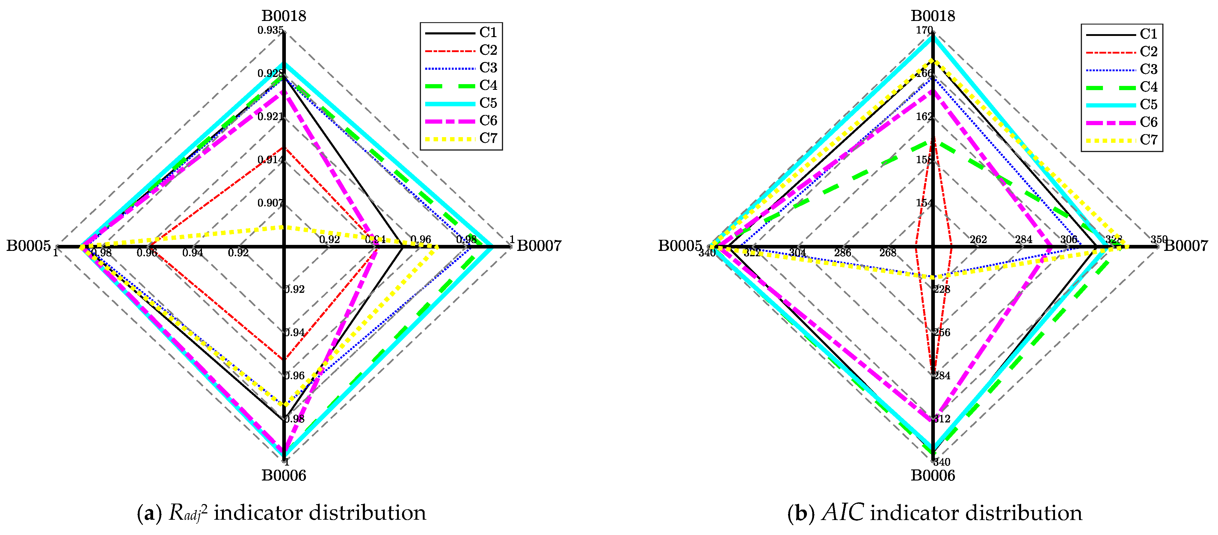
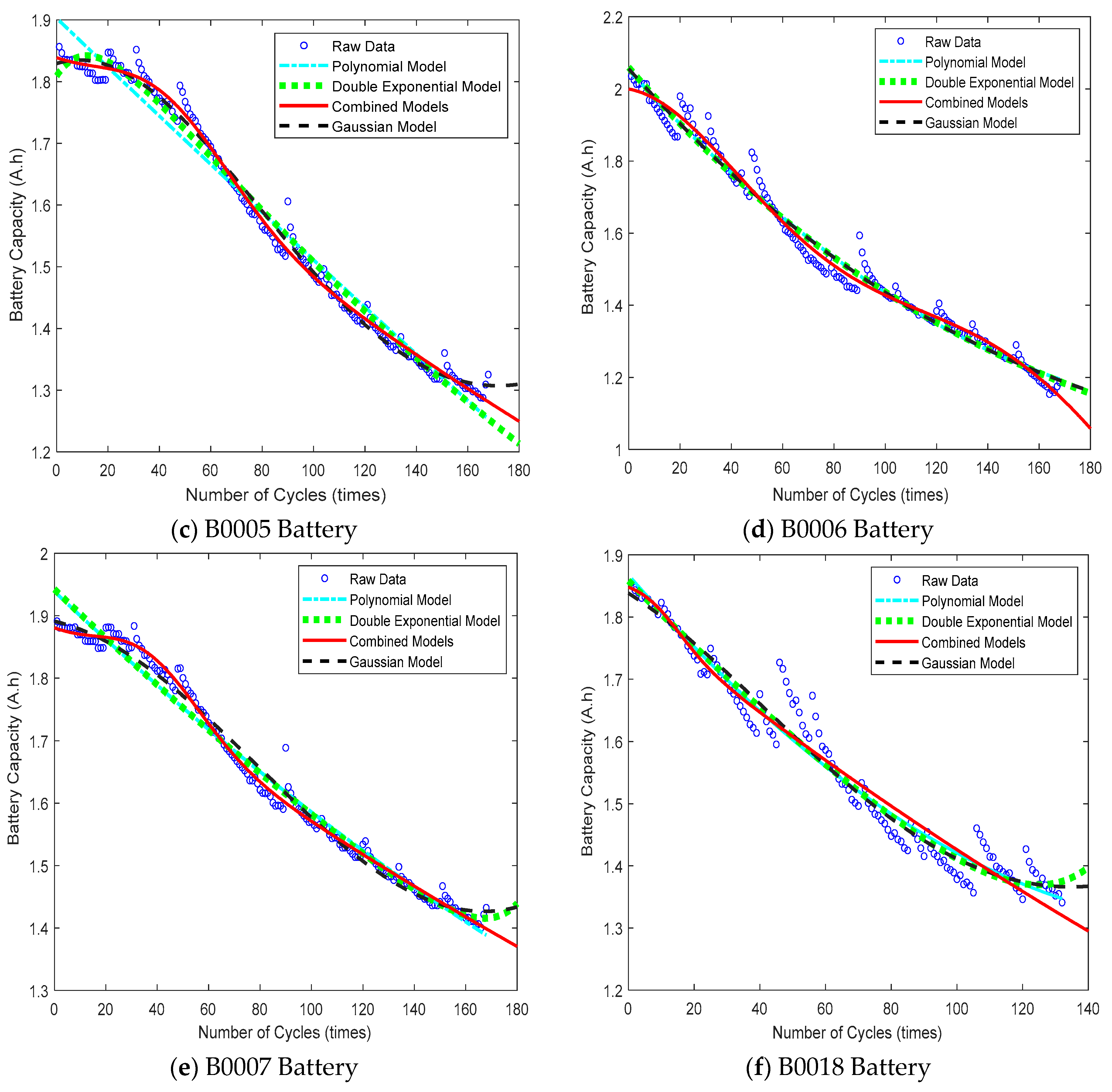
3.1. Construction of the Battery Capacity Decline Model

Due to the complex electrochemical processes involved in battery degradation, establishing an accurate model for battery degradation is challenging [24,25]. Currently, the most commonly used empirical models for battery degradation include the double exponential model based on capacity decline [26] and polynomial models [27]. Additionally, some researchers have employed Gaussian regression models [28] and other statistical approaches.

The double exponential model that characterizes the trend of battery capacity degradation is expressed in Equation (27) as follows:

$$C_{\mathrm{e}}=C_{e1}+C_{e2}=a_1\times e^{a_2\times k}+a_3\times e^{a_4\times k}$$

(27)

In the equation, C_e represents the battery capacity at the k-th cycle; k denotes the battery charge–discharge cycle; and a₁, a₂, a₃, and a₄ are the unknown parameters of the model.

The polynomial model that characterizes the trend of battery capacity degradation is expressed as follows in Equation (28):

$$C_p=C_{p1}+C_{p2}+C_{p3}=b_1\times k^2+b_2\times k+b_3$$

(28)

In the equation, C_p represents the battery capacity at the k-th cycle, while b₁, b₂, b₃, and b₄ are the unknown parameters of the model.

The Gaussian model that characterizes the trend of battery capacity degradation is represented as follows in Equation (29):

$$C_{\mathrm{g}}=C_{g1}+C_{g2}=c_1\times {\mathrm{e}}^{-({\displaystyle \frac{k-d_1}{e_1}}{)}^2}+c_2\times {\mathrm{e}}^{-({\displaystyle \frac{k-d_2}{e_2}}{)}^2}$$

(29)

In the equation, C_g represents the battery capacity at the k-th cycle, while c₁, d₁, e₁, c₂, d₂, and e₂ are the unknown parameters of the model.

The double exponential model and polynomial models have simple structures and low computational complexity; however, they fail to accurately capture the local features of battery capacity degradation, which can reduce the accuracy of RUL predictions. In contrast, the Gaussian model, which includes six unknown parameters, results in higher model complexity. To enhance the goodness of fit while achieving more accurate predictions and reducing model complexity, this study constructs a model with better fitting accuracy for battery capacity degradation by identifying key terms from the three models mentioned above. As shown in Equations (27) and (29), both the double exponential and Gaussian models contain two identical terms. Therefore, an analysis of the individual terms from both models is presented in

Table 1. A single fitted performance indicator.

Battery Model	Single Term of the Double Exponential Function Ce1		Single Term of the Gaussian Function Cg1
	Radj2	RMSE	Radj2	RMSE
B0005	0.9207	0.04189	0.9672	0.02695
B0006	0.9409	0.04527	0.9550	0.03950
B0007	0.9315	0.03853	0.9650	0.03150
B0018	0.8856	0.04053	0.9013	0.03767

.

From Table 1, it can be observed that, in the double exponential model, the single exponential term C_e1 has an R_adj² value above 0.88 and an RMSE value below 0.05, indicating that this term plays a critical role in fitting the trend of battery capacity degradation; thus, the contribution of the other single exponential term is negligible. In the Gaussian model, the single term C_g1 has an R_adj² value exceeding 0.9 and an RMSE value below 0.04, also demonstrating its crucial role in the capacity degradation process. In contrast, the polynomial model shows that, apart from the constant term, both the quadratic and linear terms are related to the battery’s cycle count.

In order to establish a battery model that better characterizes capacity degradation, this study validates and analyzes commonly used battery capacity degradation models, including the double exponential model, Gaussian model, and polynomial model. It is found that individual components within the dual-exponential and Gaussian models play crucial roles in the battery capacity degradation process. Therefore, a combined analysis is conducted by integrating these key components from the dual-exponential and Gaussian models, along with terms related to battery cycle counts from the polynomial model. This aims to construct a structurally simple yet better-fitting model for battery capacity degradation. Through analysis, seven different models, labeled C₁ to C₇, are proposed, and the C₁ to C₇ models are detailed in Equations (30)–(36):

$$C_1=C_{e1}+C_{p1}=a_1\times e^{a_2\times k}+b_1\times k^2$$

(30)

$$C_2=C_{e1}+C_{p2}=a_1\times e^{a_2\times k}+b_2\times k$$

(31)

$$C_3=C_{e1}+C_{p1}+C_{p2}=a_1\times e^{a_2\times k}+b_1\times k^2+b_2\times k$$

(32)

$$C_4=C_{g1}+C_{p1}=c_1\times e^{-{({\displaystyle \frac{k-d_1}{e_1}})}^2}+b_1\times k^2$$

(33)

$$C_5=C_{g1}+C_{p2}=c_1\times e^{-{({\displaystyle \frac{k-d_1}{e_1}})}^2}+b_2\times k$$

(34)

$$C_6=C_{g1}+C_{p1}+C_{p2}=c_1\times e^{-{({\displaystyle \frac{k-d_1}{e_1}})}^2}+b_1\times k^2+b_2\times k$$

(35)

$$C_7=C_{e1}+C_{g1}=a_1\times e^{a_2\times k}+c_1\times e^{-{({\displaystyle \frac{k-d_1}{e_1}})}^2}$$

(36)

where C₁–C₇ refer to the numbers assigned to the seven models.

To comprehensively assess the fitting accuracy and number of unknown parameters of each model, the AIC is introduced as an auxiliary criterion to balance the model complexity and fitting goodness [29]. The AIC is calculated following Equation (37):

$$AIC=2k_e-\ln (L)$$

(37)

where k_e is the number of parameters in the model; L is the value of the great likelihood function of the model.

Ln(L) is calculated as shown in Equation (38):

$$\ln (L)=-{\displaystyle \frac{N}{2}}\left[\ln (2\pi {\displaystyle \frac{{\displaystyle {\sum }_{i=1}^N{(y_g-{\widehat{y}}_g)}^2}}{N_g}}+1\right]$$

(38)

where N_g represents the number of samples; $y_g-{\widehat{y}}_g$ is the difference between the measured value and the estimated value.

The effectiveness of curve fitting can also be assessed using R_adj² from the regression analysis, which characterizes the overall fit of the regression equation, which expresses the overall relationship between the dependent variable and all independent variables [30]. Therefore, the constructed seven models are evaluated and selected using the evaluation metrics R_adj² and the AIC. Since the computed AIC values for each model are negative, a larger absolute value of AIC indicates a better fit, with R_adj² values approaching 1 indicating higher model fitting effectiveness [31]. Figure 1 shows the distribution of the seven constructed model performance indicators.

From the indicator distribution plot in Figure 1, the coordinates for B0005, B0006, B0007, and B0018 represent the battery data from the NASA publicly available Battery Data Set. The values on the axes correspond to the R_adj² and AIC values for each battery dataset within the C₁ to C₇ models. It can be observed that, compared to the other constructed models, the C₅ model exhibits the largest absolute AIC value, the R_adj² value closest to 1, and the largest area enclosed by the triangle in the plot. This indicates that the data fitting performance of the C₅ model is superior, with a lower risk of overfitting. Test data from NASA’s Battery No. 4, as well as from batteries A5 and A12, all with a rated capacity of 0.9 Ah, publicly disclosed by the CALCE group at the University of Maryland, were selected to compare the fitting performance of the constructed empirical model C₅ with three commonly used empirical models regarding battery capacity degradation trends. Evaluation metrics such as R_adj² and RMSE (root mean square error) were employed [32]. The fitting curves of the four models are shown in Figure 2a–d, and the evaluation metrics are summarized in

Table 2. Comparison of the fitting effects of the four models.

Battery Model		Radj2
		Polynomial Model	Biexponential Model	Gaussian Model	Building Model
NASA	B0005	0.9754	0.9859	0.9932	0.9930
	B0006	0.9808	0.9808	0.9859	0.9850
	B0007	0.9785	0.9795	0.9878	0.9938
	B0018	0.9587	0.9617	0.9511	0.9649
CALCE	A5	0.8776	0.9945	0.9610	0.9968
	A12	0.9529	0.9691	0.9874	0.9987
Battery Model		RMSE
		Polynomial model	Biexponential model	Gaussian model	Building model
NASA	B0005	0.0299	0.0226	0.0152	0.0150
	B0006	0.0350	0.0349	0.0300	0.0319
	B0007	0.0236	0.0230	0.0182	0.0127
	B0018	0.0314	0.0303	0.0342	0.0302
CALCE	A5	0.0359	0.0076	0.0205	0.0058
	A12	0.0581	0.0471	0.0300	0.0098

.

From Figure 2 and Table 2, it is evident that, compared to the polynomial and dual-exponential models, the constructed model C₅ demonstrates superior fitting performance across these six battery sets. Furthermore, the constructed model involves only four unknown parameters, making it simpler than the Gaussian model. Therefore, the C₅ model constructed in this study is selected for subsequent analysis as the battery capacity degradation model.

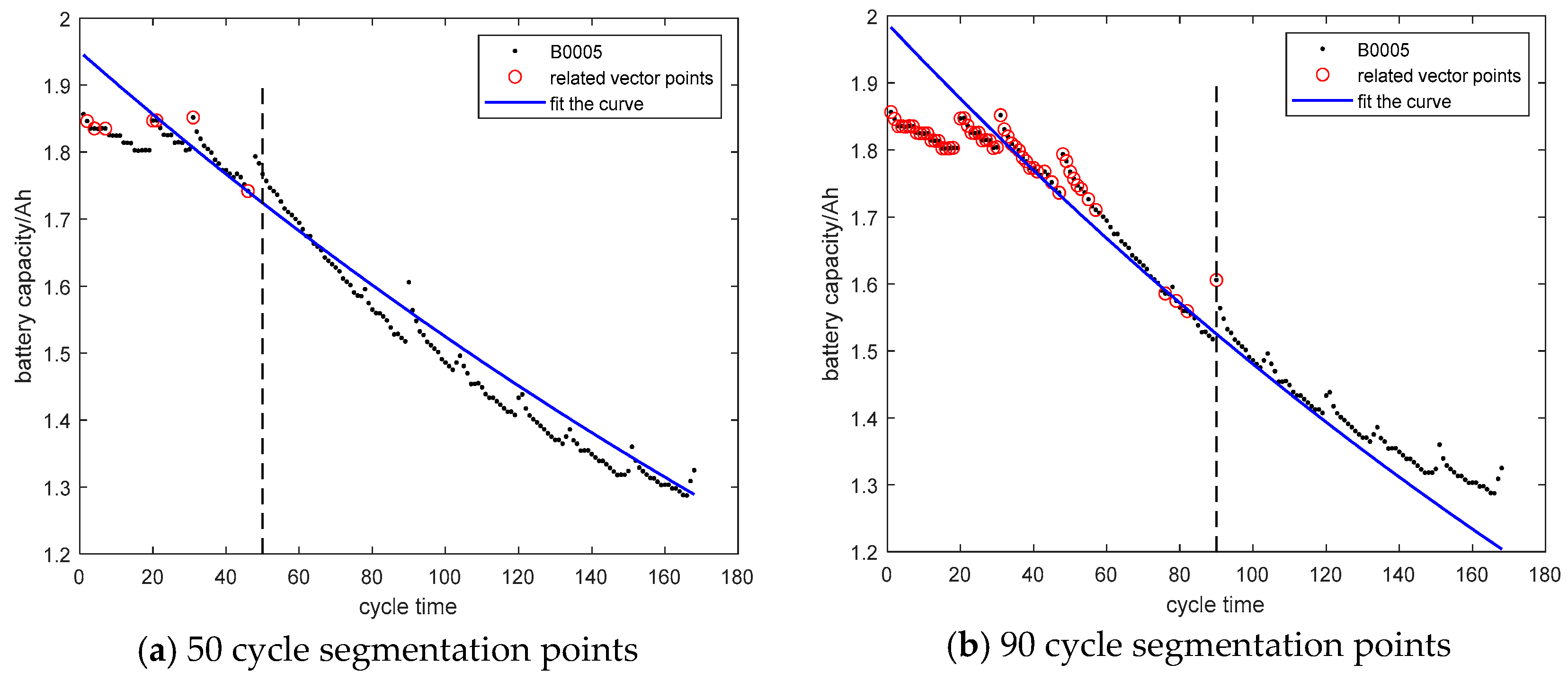
3.2. Model Initialization

PF algorithms are sensitive to the selection of initial states, because they require careful initialization. Improper initialization can lead to increased bias and variance in the algorithm, thereby affecting the estimation accuracy [33].

Currently, there are two main methods for obtaining the initial parameters for models: One method collects battery data under identical operating conditions, using all battery group data, including the battery being predicted, as a training set to train the model and obtain the model parameters and then averaging the parameters to obtain the initial parameters for the prediction battery [34]. This method is suitable for datasets of battery groups that have similar operating conditions. Its advantage lies in not relying on the battery to be predicted. However, a drawback is that each battery’s performance characteristics may vary, leading to initial model parameters that sometimes do not align with actual conditions. Another method involves splitting the data of the prediction battery into two parts: the first part is the training set, while the second part is the test set [35]. This approach typically results in training data that closely matches the prediction battery. Often, the first 30% or 70% of the data is selected as the training set, with adjustments based on the severity of battery capacity degradation in practical applications [36].

This study employed the second method to determine the initial parameters for the battery model, using battery data sourced from the NASA dataset. Due to varying cycle numbers among the battery tests, batteries B0005, B0006, and B0007 each underwent 168 cycles. Considering battery life thresholds, segments of 50 and 90 cycles were selected as breakpoints for these three battery datasets. These segments were also chosen as the starting points for prediction, with the earlier data serving as the training set and the later data as the test set. Battery B0018 underwent 131 cycles, and segments of 50 and 80 cycles were selected as data breakpoints.

The training algorithm utilizes the RVM to train the battery data and obtain feature points, specifically the relevant vector points for the battery being predicted. Subsequently, the nonlinear least squares method is employed to identify these relevant vector points, thereby identifying the four parameters of the C₅ model. Taking battery B0005 as an illustrative example, simulation results based on the RVM, using the 50th and 90th cycles as prediction start points are compared to the experimental results in Figure 3a,b.

From Figure 3a,b, it can be observed that, even with a limited amount of battery data, the model initialized using RVM can effectively track the trend of battery capacity degradation. Moreover, as the training data volume increases, the curve fitted using RVM initialization tracks the capacity degradation trend more accurately. This provides a better initial state space equation for PF algorithms.

3.3. Battery Rul Prediction Process

This paper approaches battery RUL prediction by obtaining the initial parameters for the battery capacity degradation model using RVM. Subsequently, the RP-UPF algorithm is utilized to predict the battery’s RUL.

When applying the RP-UPF algorithm to predict the RUL of batteries, the parameters of the constructed battery capacity degradation model vary throughout battery usage [37]. Therefore, the four parameters of the degradation model are treated as state variables of the observation model. The state equation and observation equation are represented by Equations (39) and (40):

$$\left\{\begin{array}{l}{a}_k=a_{k-1}+w_a\begin{array}{cc}& w_a ~ N(0,{\delta }_a)\end{array}\\ b_k=b_{k-1}+w_b\begin{array}{cc}& w_b ~ N(0,{\delta }_b)\end{array}\\ c_k=c_{k-1}+w_c\begin{array}{cc}& w_c ~ N(0,{\delta }_c)\end{array}\\ d_k=d_{k-1}+w_d\begin{array}{cc}& w_d ~ N(0,{\delta }_d)\end{array}\end{array}\right.$$

(39)

$$Q_k=a_k\cdot e^{-{((k-b_k)/c_k)}^2}+d_k\cdot k+\nu \begin{array}{cc}& \nu ~ N(0,{\delta }_{\nu })\end{array}$$

(40)

where k is the battery charge/discharge cycle period; $Q_k$ is the battery capacity measured in k cycle periods; a, b, c, and d are the battery capacity decline model parameters; w is the process noise; and $\nu$ is the measurement noise. The process noise, as well as the measurement noise, are Gaussian white noise with mean 0, and variance $\delta$ is the Gaussian white noise.

Applying the RP-UPF algorithm involves iteratively updating the model parameters until reaching the prediction starting point. The model obtained through this process represents the final model for lithium-ion battery capacity degradation.

This paper sets the lifetime threshold for a lithium-ion battery at 70% of its rated capacity and determines the remaining battery lifetime by solving Equation (41):

$$0.7Q_{rated}={\alpha }_k{e}^{(-{((L_k-b_k)/c_k)}^2)}+d_k\times RU{L}_k+w_k$$

(41)

where Q_rated is the rated capacity of the battery; RUL_k is the RUL of the battery predicted by Q_k in the k-th cycle; L_k is the value of the great likelihood function of the model in the k-th cycle.

The predicted value of battery RUL at cycle k is obtained by substituting the posterior parameters in the battery capacity recession equation into Equation (41) to solve the equation, and the PDF of the predicted battery RUL can be calculated using Equation (42):

$$P(RU{L}_k|Q_{1:k})\approx {\displaystyle \sum _{i=1}^N{w}_k^i\delta (RU{L}_k-RU{L}_k^i})$$

(42)

where ${RUL}_k^i$ is the remaining lifetime of the cell predicted by the state estimate $x_k^i$ of the i-th particle in the k-th cycle;${ x}_k^i$ is the state variable; δ is the Dirac function.

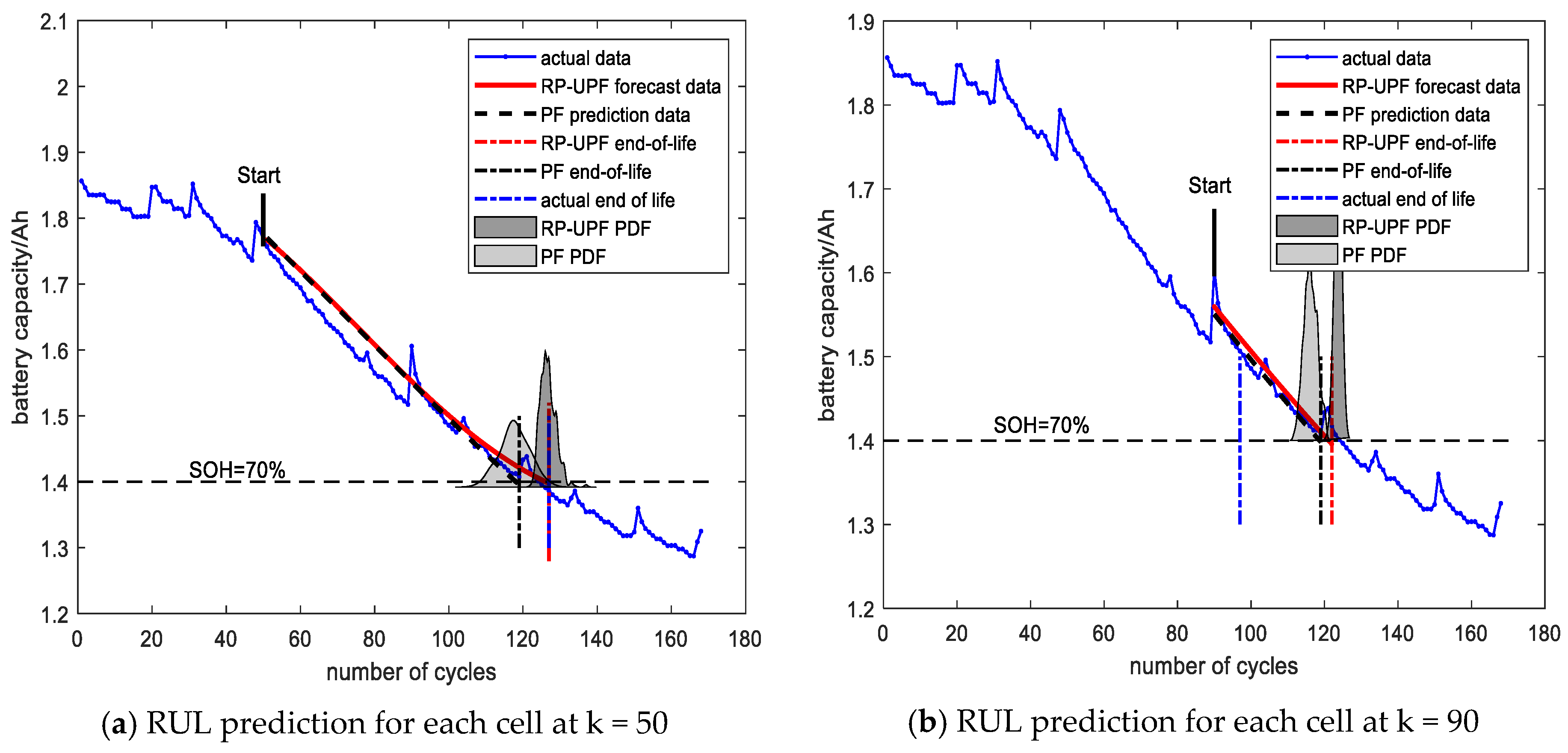
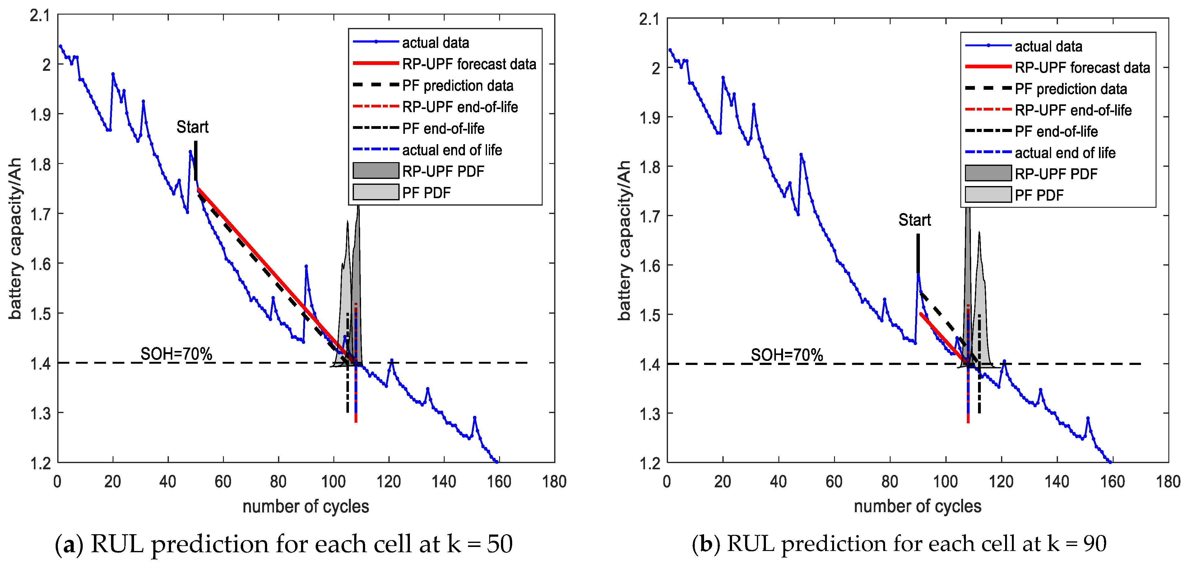
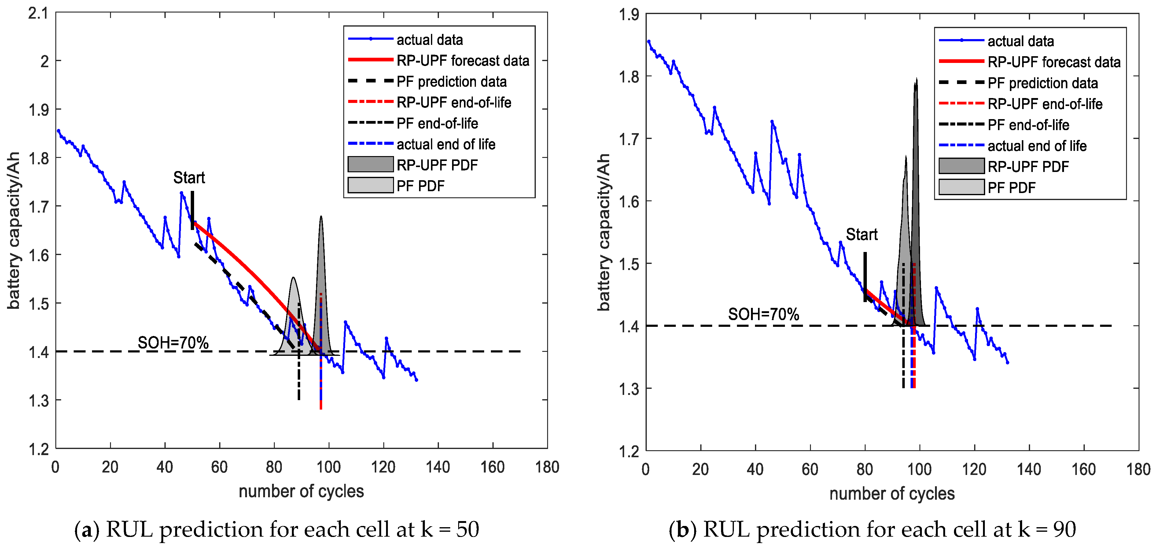
3.4. Analysis of the Battery Rul Forecast Results

To validate the performance of the model-based battery RUL prediction method during the early and late cycle periods, RUL prediction studies were conducted on NASA dataset batteries B0005, B0006, and B0018. Battery B0007 was excluded from the study because its capacity degradation did not reach the failure threshold [38]. Accordingly, batteries B0005 and B0006 were selected with the 50th and 90th cycles as the prediction start points for the early and late periods. Battery B0018 was chosen with the 50th cycle for early prediction and the 80th cycle for late prediction. The battery RUL was terminated when the capacity reached 70% of its rated capacity or 1.4 Ah. Before the prediction start point, the data were used as the training set. The initial parameters of the models obtained using RVM for the three batteries are presented in

Table 3. Initial parameter values of the RVM-based battery capacity degradation model.

Battery Model	Starting Cycle	a (0)	b (0)	c (0)	d (0)
B0005	50	1.8883	−20.6662	125.9084	0.0073
	90	1.8730	−21.5266	128.8280	0.0089
B0006	50	2.4047	−101.6399	243.6830	0.0019
	90	2.5168	−94.0786	262.3111	0.0021
B0018	50	1.9279	42.4843	205.8986	−0.0075
	80	1.8546	37.4501	373.0657	−0.0046

.

After obtaining the initial predictive model values from different starting cycles, the predictive models based on the RP-UPF and the basic PF algorithms were compared and analyzed for their effectiveness in predicting the battery RUL. The RUL prediction results using the two different filtering methods are illustrated in Figure 4 and Figure 5, with the quantitative metrics of RUL prediction effectiveness shown in

Table 4. Quantitative indicators for the evaluation of the battery RUL prediction results.

Battery Model	Start	Filtering Algorithm	Actual RUL	Projected RUL	Absolute Error	Relative Error (%)	PDF Width
B0005	50	RP-UPF	74	77	3	4.05	9
		PF		69	5	6.76	19
	90	RP-UPF	35	33	2	5.71	6
		PF		30	5	14.29	9
B0006	50	RP-UPF	59	58	1	1.69	6
		PF		55	4	6.78	7
	90	RP-UPF	19	18	1	5.26	5
		PF		22	3	15.79	8
B0018	50	RP-UPF	54	47	0	0	7
		PF		39	8	14.81	12
	80	RP-UPF	24	22	2	8.33	6
		PF		20	4	16.67	8

.

Figure 4, Figure 5 and Figure 6 show that the battery capacity degradation curves obtained using the PF and RP-UPF filtering methods generally align well with the experimental data trends, demonstrating the effectiveness of the proposed model-based prediction approach. Based on the example provided for battery B0005, using the 50th cycle as the prediction start point, the RP-UPF algorithm yielded absolute errors, relative errors, and PDF widths of 3, 4.05%, and 9, respectively. Compared to the PF algorithm, these values decreased by 2, 2.71%, and 10, respectively. When the 90th cycle was used as the prediction start point, the RP-UPF algorithm resulted in absolute errors, relative errors, and PDF widths of 2, 5.71%, and 6, respectively, which were reduced by 3, 8.58%, and 3 compared to the PF algorithm. Similar conclusions were drawn for batteries B0006 and B0018.This conclusion is compared with the results in the literature [39], where the absolute error and relative error for battery B0006 using the IPSO-GRU method, starting from the prediction time of 84, were 4% and 26.7%, respectively. In contrast, the absolute error and relative error reported in this study are smaller, and similar trends are observed for other batteries such as B0005 and B0018. Additionally, the battery RUL prediction results obtained in this study were compared to those based on adaptive models and the BAS-PF algorithm, as well as the double exponential model and UPF-GA-SVR algorithm and the PSO-ELM algorithm. The results indicate that, during the early stage of battery life degradation, the prediction accuracy of the method proposed in this paper is comparable to that of the UPF-GA-SVR method but superior to that of the BAS-PF algorithm. In the later stages of battery degradation, the predictions based on this method outperformed the other three methods. Furthermore, compared to the PSO-ELM algorithm, the proposed method achieves precise RUL predictions with limited historical data and provides uncertainty expressions for the RUL predictions. Therefore, it can be observed that the RP-UPF filtering method provides higher accuracy in predicting the battery RUL compared to PF. The PDF range is also more precise, offering more valuable insights for battery RUL prediction.

4. Conclusions

(1) To establish a model that accurately reflects the characteristics of battery capacity degradation, this study compared and analyzed the double exponential model, polynomial model, and Gaussian regression model. Utilizing the evaluation criteria R_adj² and AIC, the study selected model C₅ for constructing battery capacity degradation models based on higher fitting goodness. R_adj² and RMSE were employed as evaluation metrics for fitting effectiveness. The research findings indicate that the C₅ model exhibits superior fitting goodness compared to the polynomial model, dual-exponential model, and Gaussian model across the six battery groups.

(2) To obtain better initial values for the PF algorithm, this study divided the battery data into training and testing sets. Using RVM and nonlinear least squares, the initial parameter values of the C₅ model for battery capacity degradation were obtained. The research results indicate that the C₅ model derived from RVM can effectively track the trend of battery capacity degradation. Moreover, as the amount of training data increases, the model shows improved tracking of capacity degradation trends.

(3) To achieve battery RUL prediction and express the prediction range, this study employed a model prediction method comparing the RP-UPF and PF algorithms using batteries B0005, B0006, and B0018. The research results indicate that the RP-UPF algorithm reduces the absolute error, relative error, and PDF width compared to the PF algorithm. Specifically, for the same cycle period, the RP-UPF algorithm provides higher accuracy in battery RUL prediction and a narrower PDF range compared to the PF algorithm. This capability enhances the value of battery RUL prediction significantly.

(4) This study developed the C₅ model, which exhibits superior goodness of fit compared to the polynomial, double exponential, and Gaussian models. The initial parameter values for the C₅ model were determined using RVM and nonlinear least squares methods. Additionally, the RP-UPF algorithm was utilized to enhance traditional PF algorithms, effectively addressing the challenges related to prediction accuracy constrained by model fidelity, as well as issues of particle degradation and insufficient diversity in PF methods. This approach offers valuable insights for future battery RUL predictions.

References

1. Ding, D.; Sun, N.; Li, A.; Li, Z.; Zhang, Y. Research on vehicle battery data cleaning method based on OOA-VMD-ATGRU-GAN. Phys. Scr. 2024, 99, 045013. [Google Scholar] [CrossRef]
2. Li, Z.; Li, A.; Bai, F.; Zuo, H.; Zhang, Y. Remaining useful life prediction of lithium battery based on ACNN-Mogrifier LSTM-MMD. Meas. Sci. Technol. 2023, 35, 016101. [Google Scholar] [CrossRef]
3. Li, Z.; Bai, F.; Zuo, H.; Zhang, Y. Remaining Useful Life Prediction for Lithium-Ion Batteries Based on Iterative Transfer Learning and Mogrifier LSTM. Batteries 2023, 9, 448. [Google Scholar] [CrossRef]
4. Feng, S.; Wang, A.; Cai, J.; Zuo, H.; Zhang, Y. Health state estimation of on-board lithium-ion batteries based on GMM-BID model. Sensors 2022, 22, 9637. [Google Scholar] [CrossRef]
5. Lyu, C.; Lai, Q.; Ge, T.; Yu, H.; Wang, L.; Ma, N. A lead-acid battery’s remaining useful life prediction by using electrochemical model in the Particle Filtering framework. Energy 2017, 120, 975–984. [Google Scholar] [CrossRef]
6. Miao, Q.; Xie, L.; Cui, H.; Liang, W.; Pecht, M. Remaining useful life prediction of lithium-ion battery with unscented particle filter technique. Microelectron. Reliab. 2013, 53, 805–810. [Google Scholar] [CrossRef]
7. Guha, A.; Patra, A. Online Estimation of the Electrochemical Impedance Spectrum and Remaining Useful Life of Lithium-Ion Batteries. IEEE Trans. Instrum. Meas. 2018, 67, 1836–1849. [Google Scholar] [CrossRef]
8. Hong, J.; Lee, D.; Jeong, E.-R.; Yi, Y. Towards the swift prediction of the remaining useful life of lithium-ion batteries with end-to-end deep learning. Appl. Energy 2020, 278, 115646. [Google Scholar] [CrossRef]
9. Chang, W. Data-Driven Prediction of Li-Ion Battery Remaining Useful Life and Optimization of Fast Charging Parameters. Master’s Thesis, East China University of Science and Technology, Shanghai, China, 2019. [Google Scholar]
10. Ansari, S.; Ayob, A.; Hossain Lipu, M.S.; Hussain, A.; Saad, M.H.M. Multi-Channel Profile Based Artificial Neural Network Approach for Remaining Useful Life Prediction of Electric Vehicle Lithium-Ion Batteries. Energies 2021, 14, 7521. [Google Scholar] [CrossRef]
11. Patil, M.A.; Tagade, P.; Hariharan, K.S.; Kolake, S.M.; Song, T.; Yeo, T.; Doo, S. A Novel Multistage Support Vector Machine Based Approach for Li-Ion Battery Remaining Useful Life Estimation. Appl. Energy 2015, 159, 285–297. [Google Scholar] [CrossRef]
12. Zeng, W. State-Of-Health Estimation and Remaining Useful Life Prediction Method of Lithium-Ion Battery. Master’s Thesis, Anhui University of Science and Technology, Huainan, China, 2019. [Google Scholar]
13. Liu, D.; Luo, Y.; Liu, J.; Peng, Y.; Guo, L.; Pecht, M. Lithium-ion battery remaining useful life estimation based on fusion nonlinear degradation AR model and RPF algorithm. Neural Comput. Appl. 2013, 25, 557–572. [Google Scholar] [CrossRef]
14. Dolenc, B.; Boškoski, P.; Pohjoranta, A.; Noponen, M.; Juričić, Đ. Hybrid Approach to Remaining Useful Life Prediction of Solid Oxide Fuel Cell Stack. ECS Trans. 2017, 78, 2251–2264. [Google Scholar] [CrossRef]
15. Chen, L.; Wang, H.; Chen, J.; An, J.; Ji, B.; Lyu, Z.; Cao, W.; Pan, H. A Novel Remaining Useful Life Prediction Framework for Lithium-Ion Battery Using Grey Model and Particle Filtering. Int. J. Energy Res. 2020, 44, 7435–7449. [Google Scholar] [CrossRef]
16. Ju, F.; Du, W.; Zhuang, W.; Li, B.; Wang, T.; Wang, W.; Ma, H. Profit-Effective Component Sizing for Electric Delivery Trucks with Dual Motor Coupling Powertrain. Energy 2024, 296, 131055. [Google Scholar] [CrossRef]
17. Su, N.K.H.; Juwono, F.H.; Wong, W.K.; Chew, I.M. Review on Machine Learning Methods for Remaining Useful Lifetime Prediction of Lithium-ion Batteries. In Proceedings of the 2022 International Conference on Green Energy, Computing and Sustainable Technology (GECOST), Miri Sarawak, Malaysia, 26–28 October 2022; pp. 286–292. [Google Scholar] [CrossRef]
18. Xiong, R.; Lu, J. Preparation of Papers for IFAC Conferences & Symposia: A comparative study of remaining useful life predictions for lithium-ion battery. IFAC-Pap. 2018, 51, 268–273. [Google Scholar]
19. Zan, M.; Zhou, H.; Han, D.; Yang, G.; Xu, G. Survey of Particle Filter Target Tracking Algorithms. Master’s Thesis, School of Electronic and Information Engineering, Beijing, China, 2019. [Google Scholar]
20. Wang, H.; Peng, Z. Structural response reconstruction based on improved particle filter algorithm. Noise Vib. Control. 2023, 43, 31–37. [Google Scholar]
21. Zhang, K.; Wang, W. EKF-PF algorithm based SOC estimation of retired power lithium batteries. Mod. Electron. Tech. 2023, 46, 145–150. [Google Scholar]
22. Chen, L.; Chen, J.; Wang, H.; Wang, Y.; An, J.; Yang, R.; Pan, H. Remaining Useful Life Prediction of Battery Using a Novel Indicator and Framework With Fractional Grey Model and Unscented Particle Filter. IEEE Trans. Power Electron. 2020, 35, 5850–5859. [Google Scholar] [CrossRef]
23. Chen, W.; Cai, Y.; Su, Y.; Jiang, K.; Li, A. Remaining useful life prediction for lithium-ion battery based on improved particle filtering. China Meas. Test 2021, 47, 148–153. [Google Scholar]
24. Meng, F.; Yang, F.; Yang, J.; Xie, M. A power model considering initial battery state for remaining useful life prediction of lithium-ion batteries. Reliab. Eng. Syst. Saf. 2023, 237, 109361. [Google Scholar] [CrossRef]
25. Shi, J.; Rivera, A.; Wu, D. Battery health management using physics-informed machine learning: Online degradation modeling and remaining useful life prediction. Mech. Syst. Signal Process. 2022, 179, 109347. [Google Scholar] [CrossRef]
26. Zhang, N.; Xu, A.D.; Wang, K.; Han, X.J.; Hong, W.H.; Hong, S.H. Remaining Useful Life Prediction of Lithium Batteries Based on Extended Kalman Particle Filter. IEEJ Trans. Electr. Electron. Eng. 2021, 16, 206–214. [Google Scholar] [CrossRef]
27. Mishra, A.; Subramanian, V.R.; Suthar, B. Hexic Polynomial Approximation for Spherical Diffusion to Accelerate Accurate Lithium-Ion Battery Simulation. J. Electrochem. Soc. 2022, 169, 120532. [Google Scholar] [CrossRef]
28. Wang, S.; Li, Z.H.; Zhang, E.; Zhou, M.; Wang, K.L. State of Charge Estimation for Liquid Metal Batteries with Gaussian Process Regression Framework. In Proceedings of the 2022 International Power Electronics Conference, Himeji, Japan, 15–19 May 2022; pp. 1665–1669. [Google Scholar]
29. He, H.; Zhang, Y.; Xiong, R.; Wang, C. A novel Gaussian model based battery state estimation approach: State-of-Energy. Appl. Energy 2015, 151, 41–48. [Google Scholar] [CrossRef]
30. Duan, H.; Yi, W. Construction and optimization of EV battery capacity decline prediction model based on fusion method. Spec. Purp. Veh. 2023, 10, 8–11. [Google Scholar]
31. Xiong, R.; Zhang, Y.; He, H.; Zhou, X.; Pecht, M.G. A Double-Scale, Particle-Filtering, Energy State Prediction Algorithm for Lithium-Ion Batteries. IEEE Trans. Ind. Electron. 2018, 65, 1526–1538. [Google Scholar] [CrossRef]
32. Tang, X.; Wang, Y.; Yao, K.; He, Z.; Gao, F. Model migration based battery power capability evaluation considering uncertainties of temperature and aging. J. Power Sources 2019, 440, 227141. [Google Scholar] [CrossRef]
33. Xia, F.; Wang, Z.; Zhang, C. State of Charge Estimation of Lithium-ion Batteries with Particle Filter Algorithm. In Proceedings of the IECON 2020 The 46th Annual Conference of the IEEE Industrial Electronics Society, Singapore, 18–21 October 2020; pp. 3628–3634. [Google Scholar] [CrossRef]
34. Duan, W. Research on State Estimation and Remaining Useful Life Prediction of Lithium-Ion Batteries. Master’s Thesis, Jilin University, Changchun, China, 2023. [Google Scholar] [CrossRef]
35. Zhao, J.; Tian, L.; Cheng, C. Review on state estimation and remaining useful life prediction methods for lithium-ion battery. Power Gener. Technol. 2023, 44, 5014. [Google Scholar] [CrossRef]
36. Liao, L.; Xiao, T.; Wu, T.; Jiang, J. SOH and RUL prediction for lithium batteries based on fusion of multiple health features. Power Supply Technol. 2023, 47, 193–198. [Google Scholar]
37. Shen, Y. Hybrid unscented particle filter based state-of-charge determination for lead-acid batteries. Energy 2014, 74, 795–803. [Google Scholar] [CrossRef]
38. Cai, Y.; Yang, L.; Deng, Z.; Zhao, X.; Deng, H. Prediction of lithium-ion battery remaining useful life based on hybrid data-driven method with optimized parameter. In Proceedings of the 2017 2nd International Conference on Power and Renewable Energy (ICPRE), Chengdu, China, 20–23 September 2017; pp. 1–6. [Google Scholar] [CrossRef]
39. Wang, B.; Lei, M.; Liang, J. An IPSO-GRU-Based Prediction of Remaining Useful Life of Lithium-Ion Batteries. J. Hunan Univ. Technol. 2022, 36, 23–30. [Google Scholar]
Figure 1. Distribution of performance metrics for the seven building models.
Energies 17 05482 g001
Figure 2. Fitting curves of different batteries using four empirical models.
Energies 17 05482 g002aEnergies 17 05482 g002b
Figure 3. Comparison between simulation results and test results of the capacity of battery No. B0005.
Energies 17 05482 g003
Figure 4. B0005 battery RUL prediction results.
Energies 17 05482 g004
Figure 5. B0006 battery RUL prediction results.
Energies 17 05482 g005
Figure 6. B0018 battery RUL prediction results.
Energies 17 05482 g006