Abstract
To eliminate the flow dead zone and homogenize the asymmetric flow field of a grate furnace, spirally twisted tape inserts (STTIs) with a pitch ratio of 1.5 were installed in the vertical flues of an SCL1000-13.5/450 grate boiler. The arrangement schemes found to be present inside the chosen 1000 t/d grate furnace, determined using the orthogonal experimental method, included separate installation in chamber II, separate placement in chamber III, and simultaneous arrangement in both chamber II and chamber III. The effects of row spacing H, column spacing W, and mounting angle φ were investigated by means of the practicable and feasible numerical simulation method. With a focus on the uniformity degree of the flue gas, the results showed that temperature distribution is directly correlated with the velocity field. When it comes to the uniformity of the flow field, the exclusive use of STTIs in chamber II was better than that in chamber III. Under the optimal combination scheme of STTIs in both chamber II and chamber III (scheme N323), the exhaust gas temperature reached the minimum value and the uniformity index of temperature increased to the range of 0.994~0.997. The findings in this work could provide a reference for the optimization of the flow field in a grate furnace.
1. Introduction
Due to industrialization and urbanization, the generation of municipal solid waste (MSW) has shown an inevitable increasing trend. According to predictions, the worldwide annual generation of MSW can reach up to 2.2 billion tons in 2025 [1]. The ever-growing speed of MSW production poses a huge challenge to both developed and developing countries, especially taking land shortage into consideration. When it comes to MSW treatment, the methods of landfilling, incineration, and composting have become dominant [2].
The incineration rate has experienced a meteoric rise in the past ten years due to its effective reduction in waste volume and comprehensive utilization of waste energy [3], not to mention incentive policies implemented by the government. Applicable to different kinds of MSW, there are diverse combustion techniques, each with their corresponding strengths and weaknesses. As a result, varied combustion devices have come into use, such as grate boilers, fluidized bed boilers [4], gasifiers [5], and so on. Since 2019, over 50% of MSW has been treated under incineration in China, among which more than 85% was by grate boilers [6]. Compared with a natural gas-fueled power plant, a WtE power plant has remarkable advantages in economics, for the environment, and for society [7]. Serving as a collaborative disposal thermal device, the grate furnace adopts the layer combustion technology, which divides the combustion process into three stages: desiccation, ignition, and burnout [8]. Combustion byproducts such as ash, particles, and pollutants such as dioxins will inevitably be produced during the incineration process [9]. Take hazardous fly ash, for instance; methods such as cement-based stabilization/solidification, thermal treatment, and cement clinker co-combustion were developed for the harmless treatment of fly ash [10]. Consequently, flue gas purification, leachate treatment, and slag utilization systems were equipped with incineration systems [11]. Since the implementation of a policy for waste classification in 46 key cities in China in 2017 [12], MSW feedstock diversities have posed a great challenge to the continued operation of existing incinerators. The layer incineration technology is applicable in modernized cities with good implementation of policies on waste classification and is primarily employed by grate furnaces. A survey found that after the implementation of waste classification, the moisture content of MSW dropped by 13.6%, while the heating value increased by 16.2% [13]. At the same time, pollutant emissions, except NOX, were significantly reduced in the investigated municipal domestic waste incineration plants in Shanghai and Ningbo [14].
To better accommodate the new policy, Gu et al. [15] investigated the impact of feedstock change through the advanced CFD simulation method. That study showed that adjustments to air supply and thermal input were beneficial to boiler operation and energy recycling, which increased the uniformity of turbulent kinetic energy by 51.39% and 81.04%, respectively. Fu et al. [16] compared two methods of incineration, including the oxy-fuel incineration technology and co-incineration with the coal method. From the perspective of environment and economics, the oxy-enriched incineration method retains obvious advantages for MSW incineration in China [17]. Apart from the problems of requiring a large quantity, great variety, and disposal, industrial solid waste (ISW) also has the characteristics of a high heating value and a large flammable portion [18]. Accordingly, there is broad potential for the application of domestic waste blended with ISW, which puts forward a higher demand for grate furnaces.
The details in a flow field and smoke distribution cannot be captured by means of experimental measurements, making flow field optimization difficult to verify. With the help of the CFD method [19], the combustion process of combustible solid waste in a hearth can be simulated, gas phase compositions can be calculated, and the influence of an air distribution scheme can be studied. The coupling method of a 1D fuel bed conversion model and a 3D freeboard CFD combustion model has been commonly used and widely validated by researchers via simulation of a grate furnace [20,21]. To improve its accuracy, Shen et al. [22] applied the two-air-staged combustion technology to the formation of NOx during combustion. Netzer et al. [23] proposed a reactor network approach to predict the distribution of the gas phase released by the fuel bed. Zeeshan et al. [24] developed a combined thermodynamic equilibrium model showing better accuracy in predicting product gas composition. From the results of the parametric analysis, the equivalence ratio plays a more significant role in the model compared with gasification temperature. Morteza Taki [25] proposed machine learning models to predict higher heating values for MSW to further evaluate its physicochemical properties and thermal energy content. Vanierschot et al. [26] utilized three specific bed models for the simulation of MSW incineration grates. Compared with the whole moving bed model and the multi-zone model, the fixed bed model was suggested for industrial grate-firing systems.
To obtain higher combustion efficiencies and stability, quite a few scholars have turned to the structural optimization of grate boilers. During the design stage, the broad application of CFD methods provides abundant information for analysis, in addition to a visualization of the flow details. Wu et al. [27] researched the effects of the arrangement and cone angle of the injections as well as the inlet distance in a pyrolysis furnace. Machine learning algorithms were also used in the optimization process. Taking particle dynamics as the point, Wei et al. [28] investigated the microstructure and heat transfer characteristics of blast furnaces using CFD and DEM methods. Focused on the asymmetric combustion issue, Wei et al. [29] analyzed the effect of the furnace throat space on the flow-field deflection and NOx emissions. Yang et al. [30] designed a novel furnace throat structure for the reduction in dust particle concentration in the flue gas, which could remove 40% of the dust particles in weight.
The inhomogeneity between components of solid waste leads to higher instability of the operation process. As a result, an uneven distribution of flue gas occurs in the furnace [31], which not only brings about a temperature deviation in smoke in the horizontal flue but also exerts an adverse impact on the outlet steam temperature. Accordingly, the comprehensive performance of subsequent heat exchanger surfaces, such as superheater and reheater, will be reduced. Additionally, the lower the exhaust gas temperature is, the higher the heat transfer efficiency will be. For the sake of both security and economy, it is of great necessity to take measurements for optimizing the flow field distribution. With the advantage of easy manufacture, low cost and applicability to contaminated fluid, disturbance devices have been utilized in air preheaters and have few requirements for maintenance [32,33]. Among them, twisted tape inserts are primarily used for vortex generation and velocity distribution modification [34]. Considering the suitability of spiral structure for smoke-containing fly ash particles, in this work, an attempt was made to deploy spirally twisted tape inserts (STTIs) with a pitch ratio of 1.5 inside the domestically produced 1000 t/d grate furnace. According to findings from the published literature and engineering experience, tape inserts were installed in the vertical flues instead of the furnace throat. Arrangement schemes could be divided into separate installation in chamber II, separate placement in chamber III, and synchronous arrangement in both chamber II and chamber III. Based on the orthogonal experimental method, the effects of row spacing, column spacing and mounting angle on the uniformity of flue gas were investigated to find the optimal installation method. A qualitative and quantitative analysis of the velocity field and temperature distribution was conducted through the numerical simulation method, with a focus on the uniformity of the flow field.
2. Materials and Methods
2.1. Computational Domain of the Grate Furnace
The suitability for fuels with low heating value and high moisture content makes the grate furnace fit for MSW in China. Domestic units Shanghai SUS Environment Co. Ltd. Shanghai, China, have conducted independent research on moving grates and manufactured a 1000 t/d grate furnace named the SCL1000-13.5/450 grate boiler. The equipment has been put into use in Jiaxing, Zhejiang Province, China. It operates at a steam temperature of 723.15 K and a pressure of 13.5 MPa, respectively. The incinerator is in a horizontal π-shaped arrangement, which consists of three vertical water-wall flues. The general view of the whole incineration system is depicted in Figure 1, including the horizontal flues installed with multi-stage superheats and desuperheaters, and the steel backpass equipped with seven sets of economizers. Chamber I is outlined in blue, while chambers II and III are framed with green and purple lines, respectively. The installation area for the STTI is circled in yellow before the horizontal flues. With the purpose of investigating the flow field inside the combustion system, the computational domain is composed of the furnace throat and the vertical flues. Thermocouple probes were installed near the right-side wall of the furnace for temperature measurement, labeled T1, T2 and T3. The flow field and the temperature field were simulated through the commercial software ANSYS Fluent 19.1, and the fluid properties were set according to the feedstock characteristics, while boundary conditions were based on operating conditions. These details will be introduced in the following sections.
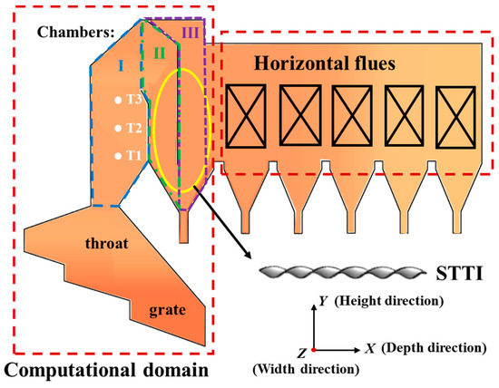
Figure 1.
A general view of the grate furnace.
The three-dimensional model is built according to the drawing, which can be divided into three furnace chambers. Regarded as chamber I, the combustion chamber is 6300 mm in depth and 11,410 mm in width, as listed in Table 1. Furnace chambers II and III are the second and third ports, respectively, where the STTIs are installed. This work made some structural simplifications to decrease the complexity of grid generation, especially on the difference between structures of the front wall and the back wall. The section depth of the former is 4830 mm, while the latter is 3850 mm. Owing to the nonlinearity of the flow field and the heat transfer process inside the incineration chamber, a full three-dimensional model structure is constructed for accurate flow rate and temperature distribution instead of a symmetrical computational field. The depth direction is defined as the x-axis and gas flows along the positive direction, while the height direction is the y-axis and the width direction is the z-axis. The lowest point of the grate furnace is set as y = 0 mm and the center section as z = 0 mm. In a gesture to avoid the backflow, an eight-meter-long structure is extended at the outlet of the incinerator model.

Table 1.
Main particulars of the grate furnace.
2.2. Grid Generation and Boundary Condition
The schematic diagram of grid generation is displayed in Figure 2. For high-quality meshes, the grate furnace model is partitioned into different blocks. Nozzles and correlated parts of the boiler are discretized with unstructured tetrahedral mesh while the others are discretized with a hexahedral mesh. Taking the disparity of dimension between nozzles and chambers into account, the secondary air nozzles and the recycled flue gas nozzles are adopted with grid refinement. The minimum and maximum grid sizes are about 20 mm and 145 mm, respectively.
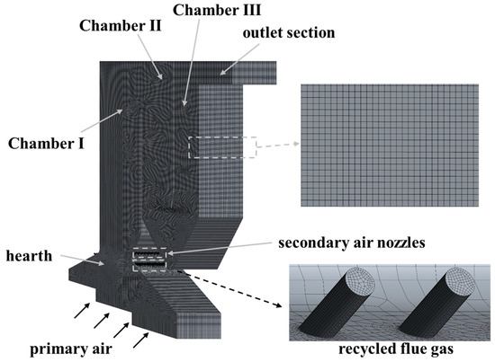
Figure 2.
A schematic view of the grid generation method.
The often-used meshes for discretization of large-scale utility boilers [35] are about 1–2 million grids. The results of grid independency are presented in Figure 3, demonstrating the velocity of flue gas along the height direction in chamber III. The grid discretization method with a number of 5.47 million is considered to be dense enough. Further mesh refinement makes no remarkable difference to the numerical results.
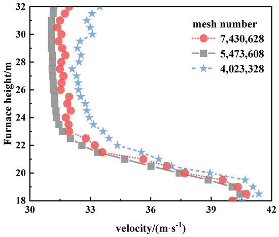
Figure 3.
Results of grid independence study.
Given the moving velocity of grates, the gradients of feedstocks, the temperature of primary air, and other parameters such as conditions of the solid phase could be obtained according to equations from the published literature [36,37], as well as the temperature distribution along the grate length direction. It has been proved that [38] the impact of the grate inlet conditions is mainly restricted in the primary chamber, which will be largely attenuated after injection and the mixture of secondary air and tertiary air. For simplification, the temperature boundary condition is assigned to the fluid domain through the User-Defined Function (UDF), as depicted in Figure 4. The temperature rises sharply when the volatiles begin to release and reaches the maximum value of 1356.41 K near 7.8 m in the length direction, where moisture in the combustible solid waste basically evaporates. With the decrease in the release rate, the temperature gradually drops and stabilizes to about 596.54 K, where volatiles are almost released in the burnout section. The heat generated in the combustion process can be calculated via a theoretical formula and imported as the source term for boundary conditions.
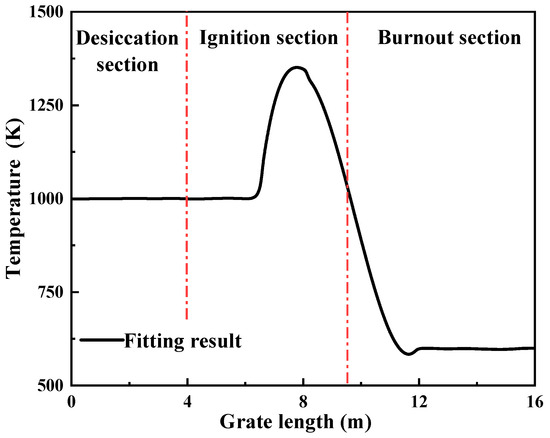
Figure 4.
Fitting curve of the grate temperature.
During simulation, the moving grate is set as velocity inlet, together with the inlet of nozzles. The extended outlet part is set as a pressure outlet. For simplification, the wall of the hearth applies the adiabatic boundary condition, while the water wall around the furnace is treated as the constant wall temperature condition. All of them meet the no-slip boundary condition. The length of the desiccation stage is 4.04 m, while that of the ignition stage and the burnout stage is 5.40 m and 6.72 m, respectively. According to the engineering application, the excess air ratio is 1.7 for the condition of Maximum Continuous Rating (MCR). The primary air is transmitted according to the air distribution, which is in the total air volume of 115,260 m3/h with a temperature of 453 K. The secondary air with a temperature of 293 K is fed into the furnace throat by nozzles in the volume of 9500 m3/h.
2.3. Simulation Model and Fluid Properties
When it comes to turbulent mixing, the realizable k-ε turbulence model proves its suitability for engineering applications. By referring to the published literature [39], the Discrete Ordinates (DOs) radiation model is utilized for radiative transfer, and the weighted sum of gray gases model (WSGGM) is adopted for evaluating the gas absorption coefficient in this work. To solve the coupling equations of pressure and velocity, the SIMPLE algorithm is used with the application of the second-order upwind discrete scheme for control equations. In terms of computational difficulty and actual requirement, the deposition of particles in the incinerator is not taken into consideration.
In reality, the measured gas components of incineration exhibit dramatic differences for each time. Therefore, the theoretical gas composition of designed feedstocks after complete combustion is deployed as the input, instead of the averaged values for three times. Table 2 illustrates the constituents of combustible solid waste under three different working conditions of the SCL1000-13.5/450 grate boiler. In this work, the corresponding low heating value of feedstock is 7955 kJ/kg at the MCR condition.
Table 2.
Characteristics of feedstock under different working conditions.
The composition of the flue gas can be obtained on the premise of complete combustion and corresponding physical property parameters can be set under different temperatures, as elucidated in Table 3. The working medium is incompressible smoke.
Table 3.
Components of flue gas after complete combustion.
2.4. Initial Flow Field and Validation
In a gesture to determine the installation location of the disturbance device, a specific analysis should be carried out on the initial flow field of flue gas. It is worth noting that the non-uniformity is amplified due to the structural simplification. According to the boundary conditions described above, the temperature distribution inside the grate furnace can be displayed as in Figure 5. During the process of flue gas flowing upward in the vertical direction until entering chamber III, a drop in temperature and improvement in uniformity of the temperature field can be observed. The temperature of the center section in width (z = 0 m) is different from that near one side of the grate wall (z = 5.705 m). The injection of secondary air and recycled flue gas brings about perturbation to the airflow in the furnace, which lowers the temperature near the front and rear walls as a consequence.
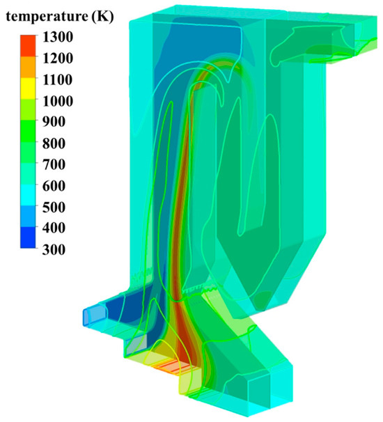
Figure 5.
Initial flow field of temperature.
The above-mentioned thermocouple probes T1–T3 (depicted in Figure 1) are installed at heights of 24.4 m, 21.6 m, and 18.2 m, respectively. Three tensors are mounted at a certain height along the width direction. In comparison with simulation results, the average value of measured temperature at each cross section is used for validation. During experiments, the working conditions comply with the operating instructions, which are identical to those of the simulation. The heating value of MSW is a bit lower than 7955 kJ/kg. It is worth noting that the presence of ash deposits distributed on the surface of the thermocouple could lead to a deviation in the measurement of approximately ±10 °C. From Table 4, all of the relative errors are in the range of ±5% as an indicator of reliability and precision for the simulation method.
Table 4.
Comparison of temperature at measuring points.
From the streamline of the center section in the width direction illustrated in Figure 6, the flue gas is transferred to the hearth from the bottom of the grate, at the set speed as the inlet boundary condition. As labeled with a blue box, the flow dead zone emerges on the side near the hearth, while the flue gas flows into chamber II. Such a phenomenon reappears under the action of inertia when the fluid flows into chamber III from the bottom corner of chamber II. As a result, the continuous impact of fly ash particles on certain heating surfaces will result in concentrated wear. On the other hand, non-uniform temperature or even local overheating will exert an adverse effect on the service life of the furnace. From the perspective of the depth direction, it is likely to spot the inhomogeneity of the flow field. Based on engineering experience, disturbance devices are usually located at vertical flues. In order to change the flow direction and decrease the overall fluid speed, it is practicable to install tape inserts in the regions framed by the red circle. The uniformity of the flow field and the temperature distribution will be improved after the insertion of STTIs. Accordingly, the wear of the heating surface will be reduced and the service life of the furnace will be extended.
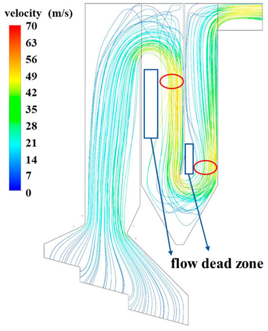
Figure 6.
Streamlines of the flue gas.
The non-uniformity also exists in the width direction, which is evaluated with the dispersion coefficient CV. The definition is given in Equation (1), written as the ratio of the standard deviation to the average value, and the physical quantity can be velocity or temperature. The larger the value is, the higher the degree of non-uniformity will be.
where σV stands for the standard deviation of a specific physical quantity; xi represents the local value and n indicates the number of measuring points.
After extraction of data on the interface between chamber III and the extended outlet section for analysis, the dispersion coefficients of velocity and temperature are 21.02% and 1.43%, respectively, without the insertion of STTIs. For a more intuitive comparison, the uniformity index of flow field γ is selected to reflect the uniformity of temperature distribution instead of CV,T. With the increase in γ, the distribution of fluid on the designated section becomes more uniform. To put it another way, physical quantity will be in the state of uniform distribution under the circumstance of γ = 1.
3. Results
Three schemes for the arrangement of STTIs are introduced in this work, including separate installation in chamber II, separate placement in chamber III, and simultaneous arrangement in both chamber II and chamber III. An orthogonal experimental method is adopted with the help of a numerical simulation method to achieve the optimal installation scheme.
3.1. Design of Orthogonal Experimental Method
Given the length and pitch ratio, the geometry of STTI is modeled by means of the 3D modeling software Solidworks 2015. Three columns and three rows of tapes are inserted in the single chamber. For convenience, the distance between adjacent STTI in the width direction (z-axis) is defined as the column spacing, expressed as W, while that in the height direction (y-axis) as row spacing H. Additionally, the angle between the centerline of tape inserts and the depth direction (x-axis) is designated as the installation angle φ, as illustrated in Figure 7. Taking the complexity of the structure into account, an unstructured tetrahedral mesh is deployed for grid discretization of STTI.
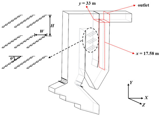
Figure 7.
A schematic view of the installation of STTIs.
Column spacing, row spacing and installation angle are selected as influence factors, corresponding to symbols A, B, and C successively. Each factor includes three different levels as presented in Table 5. As can be seen in Table 6, the orthogonal array is listed, which decides the configuration of STTIs inside chambers.
Table 5.
Influence factors and corresponding levels.
Table 6.
Conditions of the orthogonal experimental method.
3.2. Analysis of Separate Installation in Chamber II
Under the condition of separate installation in chamber II, nine specific configurations discussed in this section are denoted as ‘N12~N92′ in Table 7, while N0 represents the case without STTI. It is worth mentioning that the first row of tape inserts is mounted at a height of 29 m, with the second column at the center section in the width direction. Other tape inserts are arranged according to the row spacing, column spacing and installation angle introduced in Table 7. Focused on the outlet section, simulation results can be obtained with dispersion coefficients for evaluation. Among nine specific configurations, when STTIs are placed with a row spacing of 1.5 m and a column spacing of 2 m at an installation angle of 30°, the velocity dispersion coefficient reaches the smallest value of 0.1866. In other words, the uniformity of the flow field shows visible improvement when choosing the arrangement scheme of N12. From the perspective of the temperature dispersion coefficient, the result of scheme N12 is 5.03% higher than that of scheme N62. Although the temperature distribution is in direct connection with the velocity field, the complexity of thermal boundary conditions determines that taking mere velocity or temperature as an evaluation indicator is insufficient for the comprehensive performance of the grate furnace.
Table 7.
Numerical results of the outlet based on orthogonal experimental method.
Adding simulation results corresponding to levels 1, 2, and 3 of each influence factor into the sum, K1, K2, and K3 and correlative average values k1, k2, and k3 can be obtained. Then, the range R can be calculated to describe the impact of row spacing, column spacing and installation angle. Ordered by the value of the range as revealed in Table 8, it can be observed that the column spacing plays a significant role in the uniformity of the flow field, followed by the installation angle and the row spacing in turn. In terms of the temperature dispersion coefficient, the degree of influence concerning three influence factors is in the sequence of C > B > A. Through comparison of correlative average values, all of them reach the minimum value at level 1. Taking the homogeneity of the velocity field into account, the best combination method is A1B1C1, written as experimental scheme number N12. It is consistent with the condition concerning the temperature distribution. Therefore, the STTI should be arranged with a row spacing of 1.5 m and a column spacing of 2 m at an installation angle of 30°.
Table 8.
Results of range analysis under the condition of separate installation in chamber II.
Selecting the optimal configuration method (N12) and comparing it with the case without STTI (N0), Figure 8 illustrates the transformation of average velocity on the left side and the right side, which also reflects the flow condition of flue gas. The vertical coordinate represents the average value of velocity. Also worth noting is that the flow direction is identified as the positive direction of the horizontal coordinate. The grey line stands for the value of the left side (10.90 m < x ≤ 13.24 m) and the red line for the right side (13.24 m < x ≤ 15.58 m) of chamber II. From the top of the flue, which is regarded as the starting point of the horizontal coordinate, the velocity of flue gas on the right side increases rapidly in the 5 m long distance. Owing to the existence of the corner connecting chamber I and chamber II, the fluid velocity on the left side of the center section in depth reaches the peak and drops rapidly, which coincides with Figure 5.
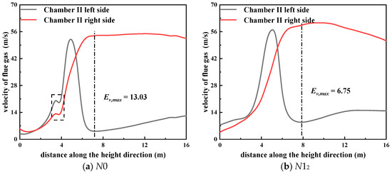
Figure 8.
Average velocity in two sides of chamber II.
At diverse heights, both sides of the cross section correspond to different average values of physical quantities, which can be written as xL and xR. Defined as , the deviation ratio Ex is utilized to reflect the uniformity of the flow field. A larger value implies more serious unevenness. In the initial case without STTI, the maximum velocity deviation ratio Ev reaches 13.03 because the flow rate of flue gas on the right side almost remains the same below a certain height. When STTI is arranged with a row spacing of 1.5 m and a column spacing of 2 m at an installation angle of 30° (scheme N12), the maximum value of the velocity deviation ratio between the right side and the left side is 6.75. The 48.20% reduction indicates an improvement in the uniformity of the flow field. Additionally, it can be perceived that a temporary fluctuation occurs in curves of velocity as marked with a dashed box in Figure 8a. The discontinuous increase in velocity can be attributed to the existence of the flow dead zone, behind which a decline in velocity occurs. Such variation flattens out with the application of STTIs.
Separate installation in chamber II not only exerts influence on the flow field of the current chamber but also makes a difference to that of the succeeding chamber. Taking the center section chamber II (x = 17.58 m) in the depth direction as the separatrix, Figure 9 demonstrates the transformation of average velocity along the flow direction, which does not take the flow direction into account. It can be seen that velocity appears in a downward trend in the flow process from chamber II to chamber III, with an average velocity of the right side (17.58 m < x ≤ 19.43 m) above 60 m/s and that of the left side (15.73 m < x ≤ 17.58 m) below 20 m/s. By comparison, the existence of STTI accelerates the flow disturbance and increases the average velocity. The positions where the maximum value of the velocity deviation ratio occurs are labeled with dotted lines. From the perspective of the velocity deviation ratio, the maximum value can reach 4.16 without the adoption of the STTI. After a separate arrangement in chamber II as scheme number N12, Ev,max declines to 3.67. The discrepancy between average velocities on two sides narrows, as seen in Figure 9b. The velocity on the left side undergoes an acceleration of 27.83% compared with that in Figure 9a.
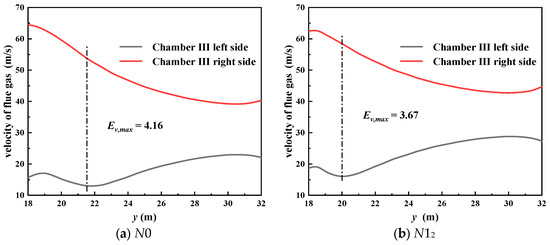
Figure 9.
Average velocity in two sides of chamber III.
Long-term operation at high temperatures increases failure probability and accumulates more fly ash particles. Apart from the velocity field, the temperature distribution also alters during the flow process in chamber III from the bottom to the top. The temperature contours of Figure 10 intuitively reflect an alteration in the top section of chamber III. No tape being inserted in chamber III notwithstanding, separate installation in chamber II brings down the average temperature of chamber III to 584.19 K. Hence, reasonable use of STTI is beneficial to prolong the service life and promote heat transfer efficiency.
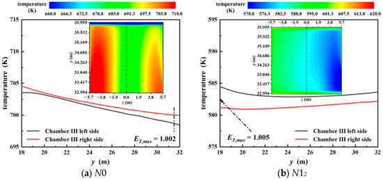
Figure 10.
Temperature distribution in two sides of chamber III.
In addition to the depth direction, inhomogeneities of velocity and temperature also exist in the width direction. As displayed in Figure 10, the position where the maximum value of the temperature deviation ratio occurs is also marked with dotted lines. The front half of the diving line (z = 0 m) has a higher temperature than the back, which will give rise to uneven distribution of temperature in subsequent heating surfaces such as the superheater. The general reason for flue gas temperature deviation can be attributed to the local velocity misalignment. For a more intuitive comparison, the local temperature at representative positions is provided instead of the average temperature. Figure 11 depicts the variation in velocity and temperature along the width direction in chamber III, where the solid line represents the value at z = −2.85 m (the front side) and the dashed line at z = 2.85 m (the back side). Simulation results of schemes N12 and N92 are plotted. The former presents a smaller deviation in both velocity and temperature than the latter, which accords with the conclusion that the best configuration corresponds to scheme N12. Additionally, there is little difference between the locations of maximum velocity in the front and the back side, as well as that of the thermal peak. From Figure 11, fluid on the front side reaches the maximum velocity at y = 15.95 m, while the highest speed is detected at y = 16.40 m on the back side. For the sake of inertial force and centrifugal force, the junction connecting chamber II and chamber III amplifies the uneven degree of flue gas, which originates from chamber II. Consequently, separate installation of STTIs can make an improvement to the flow field in chamber III.
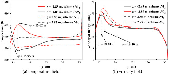
Figure 11.
Flow field conditions of chamber III along the width direction.
3.3. Analysis on Separate Installation in Chamber III
Different from the scheme of separate installation in chamber II, in this section, the mounting height of the first row is y = 21 m. Specific configurations are determined in relation to the row spacing, the column spacing, and the installation angle, assigned as ‘N13~N93’. Simulation results of dispersion coefficients about velocity CV,v and temperature CV,T in the outlet section are listed in Table 9. Among these data, evaluating indicators about velocity achieves a minimum of 0.2196 with a row spacing of 2 m and a column spacing of 4 m at an installation angle of 30° (scheme N63). Under this circumstance, the temperature dispersion coefficient also attains the minimum value of 8.752 × 10⁻³.
Table 9.
Numerical results of outlet with STTI installed in chamber III.
As the above preliminary comparison with data value is insufficient, a range analysis is carried out to calculate the range R = max(K1, K2, K3) − min(K1, K2, K3), as indicated in Table 10. For the velocity field, ranges concerning three influence factors satisfy the relation of RB > RA > RC. To put it another way, the column spacing plays the most significant role in the homogeneity of velocity in the outlet section while the installation angle is the least influential. When it comes to temperature, the ranking result of the effect exerted by influence factors is A > B > C. The minimum value of CV,v is achieved at level 1 of influence factor A, with level 3 of influence factor B and level 1 of influence factor C. The same conclusion can be drawn in terms of the temperature dispersion coefficient. Hence, the best combination method is A1B3C1, which is not comprised of nine configurations in Table 9 and is expressed as N103. The result under the circumstance of H = 1.5 m, W = 4 m and φ = 30° should be compared with that of scheme N63.
Table 10.
Results of range analysis on the outlet section.
Great emphasis is placed on the flow conditions of the flue gas in chamber III, the variation in which along the width direction is illustrated in Figure 12. After dividing the center section in depth into front and back sides by a line of z = 0 m, comparisons can be made concerning velocity and temperature. The grey curve stands for the numerical results of scheme N63, while the red one stands for scheme N103. Since no STTI is arranged in the preceding chamber to alter the fluid distribution, the variation tendencies of velocity along the height direction are basically identical. The peak value emerges at y = 15.95 m, after which the value decreases and stays almost invariant at a specific height. When flue gas flows close to chamber III, velocity will drop to zero due to the shift of flow direction. In the middle section with a constant value, the divergence of velocity between the front and back sides is 0.21 m/s for the case of scheme N103 and only 14.23% of the value corresponding to scheme N63. In general, the temperature distribution appears good following behaviors of the flow field. Analogous trends can be viewed in Figure 12b. When STTIs are mounted with a row spacing of 1.5 m and a column spacing of 4 m at an installation angle of 30°, the temperature difference between the front and back sides is only one-tenth that of scheme N63. From the perspective of the flow field in the width direction, the combination method A1B3C1 has better effectiveness in improving the uniformity.
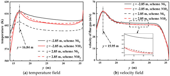
Figure 12.
Flow field conditions of front and backsides in chamber III along the width direction.
To undertake a comprehensive analysis of flow conditions in the width direction and the depth direction, various sections are extracted at different heights in both chamber II and chamber III. Substantial variation along the depth direction in chamber II is perceived in Figure 13, with less than 20 m/s on the left side and over 60 m/s on the right. Separate installation of STTIs in chamber III will make a difference to the flow field of the junction connecting chamber II and chamber III. With the adoption of scheme N103, the velocity distribution in this area is more uniform. Although the installation position is at the lower part, the uneven degree of velocity decreases through the upward flow process of flue gas in chamber III. Furthermore, the impact on the heating surface is lessened on both sides of the chamber. Therefore, the installation of STTI can optimize the subsequent flow field.
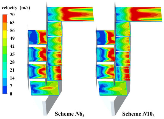
Figure 13.
Comparison of gas flow with STTIs installed in chamber III.
The flow situation of the outlet section determines the initial status of flue gas entering the horizontal flue. Consequently, it could be utilized to deduce the homogeneity of fluid in the grate furnace. The velocity field and the temperature distribution at the outlet section with the application of schemes N63 and N103 are displayed in Figure 14. In the case of combination method A1B3C1, flue gas at two sides of the center line at a width z = 0 m tends to be distributed symmetrically in the contour of velocity. The presence of a thermal peak is more off-center in the width direction for scheme N63, indicating a dramatic flue gas temperature deviation. Extracting values of velocity and temperature along the center line in height at the outlet section, a more uniform distribution of temperature can be observed near the top region of the chamber. Generally, scheme N103 has a distinct advantage in homogenizing the flow field.
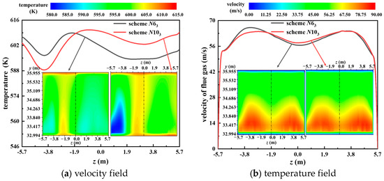
Figure 14.
Flow field conditions of outlet along the width direction.
3.4. Analysis of Concurrent Arrangement in Chamber II and Chamber III
As mentioned above, the tape insert will make a difference to the succeeding flow field. In this section, an attempt is made to set up STTI in chamber II and chamber III concurrently. Given the results of scheme ‘N123~N923’, STTIs are mounted at the height of y = 29 m, y = 27.5 m and y = 26 m in chamber II, respectively. The center lines of the three columns are located at z = −2 m, z = 0 m and z = 2 m in the width direction, with an installation angle of 30°. On this premise, the first row of STTIs is arranged at the height of y = 22 m in chamber III, slightly beyond the installation position in Section 3.3. Other than dispersion coefficients, the exit temperature, the outlet velocity, and the pressure drop are also selected as evaluation indicators. Smaller values of these parameters are preferred for better performance.
A decrease in exhaust gas temperature is considered one of the main standards for appraising thermal efficiency, which is closely bound up with the exit temperature of chamber III. From the data listed in Table 11, minimum values of all evaluation indexes can be obtained in the case of scheme N323. When STTIs in chamber III are mounted with a row spacing of 1.5 m and a column spacing of 4 m at an installation angle of 60°, the exit temperature is 568.53 K—at least 15 K lower than that of other configurations.
Table 11.
Numerical results of outlet with STTIs installed in chamber II and chamber III concurrently.
The tendency chart of various factors at different levels is plotted in Figure 15 on the basis of range analysis; thus, an intuitive comparison can be drawn between the effects of influence factors at three diverse levels. In the context of level 1 for influence factor A, with level 3 for influence factors B and C, dispersion coefficients of velocity and temperature achieve the minimum value, together with the exit temperature, the outlet velocity, and the pressure drop. In other words, the optimal test scheme should be the combination method of A1B3C3, which coincides with the conclusion of the preliminary analysis.
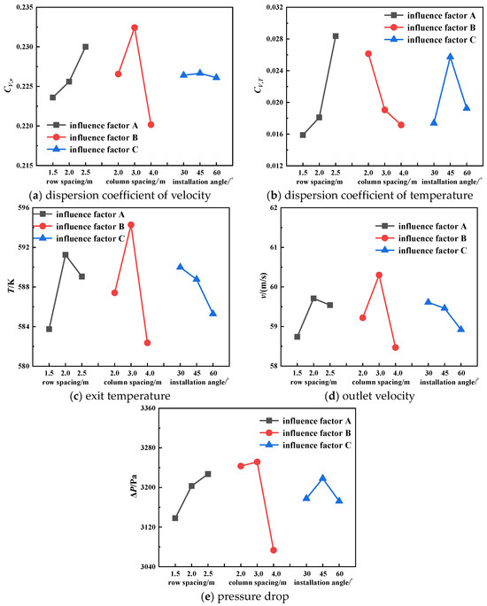
Figure 15.
Tendency chart of various factors at different levels.
Seeing the disparity of significance between the five evaluating indicators, the matrix analytical method is applied to calculate weight matrixes for the determination of the optimum solution. Relevant procedures are as follows:
- Build layer matrix M based on average indicator values kij of influence factor i at level j. Given that smaller values of indicators are in conformity with better optimal effect, reciprocals are taken as kij = 1/kij. After summarizing kij at various levels, the layer matrix of factor T can be obtained as . Concerning range Ri of influence i, a layer matrix of level S consisting of can be constructed. Taking the dispersion coefficient of velocity as an instance, calculation results of layer matrixes are as follows:
- With the definition of weight matrix as the multiplication, it can be expressed as ω1 = M1T1S1. Here, taking the dispersion coefficient of velocity as the indicator, after substituting values in step one, we can obtain
- The global weight matrix is the average value of weight matrixes concerning five different evaluating indicators . According to calculated data, the result is
According to an analysis of calculation results, the ranking result of impact made by influence factors is B > A > C. The maximum weight can be attained when level 1 is taken for influence factor A, with level 3 for influence factors B and C, corresponding to the combination method A1B3C3. Consistent with the preceding conclusion, STTIs in chamber III should be arranged with a row spacing of 1.5 m and a column spacing of 4 m at an installation angle of 60°, for the sake of optimal effects. To summarize, optimum test schemes for separate installation in chamber II and chamber III are N12 and N103, respectively, while that for concurrent arrangement in chamber II and chamber III is N323.
It is worth mentioning that the temperature difference between the left and right sides can exceed 10 K in the same chamber. Hence, great emphasis is laid on the flow field in the width direction. Figure 16 illustrates the variation in velocity and temperature during the flowing process, where test schemes N323 and N103 are compared. With regard to the velocity of flue gas, a slower speed is achieved with the adoption of scheme N323, which gives rise to a smaller velocity difference between the two sides. The same conclusion also applies to the temperature distribution. When arranging STTIs according to the scheme N323, the average temperature difference in the width direction is 3.99 K—50.6% lower than that of N103. Taking dispersion coefficients of velocity and temperature for assessment, a decreasing trend can be observed in the non-uniformity of the bottom-to-up flow in chamber III. Before flue gas is transferred from the vertical flue to the horizontal flue, values are in a steady uptrend in Figure 16c, while the transformation in temperature is behind that of velocity. The corresponding values of scheme N323 are smaller in contrast to scheme N103, including the velocity dispersion coefficient CV,v and the temperature dispersion coefficient CV,T.
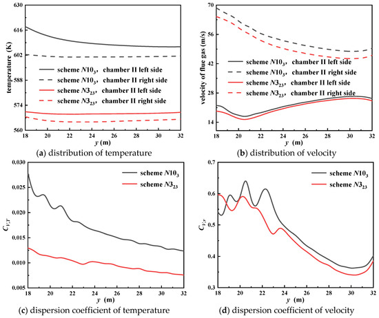
Figure 16.
Flow field conditions of different schemes in chamber III along the depth direction.
In order to discover the specific influence of installing STTIs in chamber III, an analysis of the flow field of the outlet section is also worth undertaking. The curves in Figure 17 reflect values at the center line in the height direction, where red stands for scheme N323 and grey indicates scheme N12. With respect to the velocity of flue gas, the low-velocity region is concentrated in the range near z = 0 m. From Figure 17a, a depression in the middle with bulges on both sides is detected. Additionally, separate installation in chamber II is more effective in improving the inhomogeneity of gas distribution. The velocity distribution lays the foundation of the temperature field analysis. More attention is paid to variation in temperature distribution in the optimization process, which is directly correlated with the service life and operation efficiency of the grate furnace. With the implementation of STTI in chamber III under the optimal configuration, the exhaust gas temperature decreases by about 14.78 K.
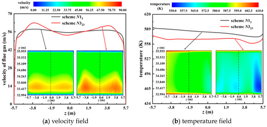
Figure 17.
Comparison of flow field conditions on the outlet along the width direction.
A comparison is made between the flow field of three optimal test schemes under different conditions in contrast to that without the arrangement of STTIs. To exclude the influence of magnitude, uniformity indexes of the flow field concerning velocity and temperature are chosen to demonstrate the variation process of flow, as shown in Figure 18. The larger uniformity index of temperature γT indicates a more uniform distribution of temperature in the depth direction. As is vividly shown in Figure 18a, the most distinct advancement takes place to the evenness of velocity when STTIs are installed separately in chamber II, with a row spacing of 1.5 m and a column spacing of 2 m at the installation angle of 30°. Scheme N323 introduces tape inserts to chamber III. Under the optimal configuration, although no significant improvement is observed, the uniformity index of temperature increases to the range of 0.994~0.997. The existence of tape insert plays a proper role in optimizing the distribution of flue gas, especially in the depth direction.
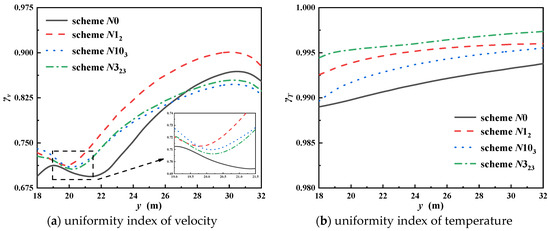
Figure 18.
Comparison of uniformity indexes in chamber III along the depth direction.
The optimization of the flow field is related to operational safety and economic efficiency. Various sections at different heights in both chamber II and chamber III are extracted in Figure 19 to display the transformation of temperature. The lower the temperature of the flue gas, the more the heat will be transferred to the heating surface. At the same time, more steam will be generated together with better waste heat utilization. In the initial flow field without tape insert (scheme N0), it can be found that the temperature of most regions exceeds 650 K, which even reaches up to 700 K. A lower temperature can be achieved with the implementation of scheme N12 compared with that under the condition of scheme N103. On the premise of separation installation, STTI can be mounted in chamber II at the distance of 29 m, 27.5 m and 26 m from the bottom. For the sake of utility maximization, the spacing between the adjacent center of columns should be 2 m in the width direction, with an installation angle of 30°. As long as conditions allow, three columns of STTI can be arranged simultaneously in chamber III at the height of 22 m, 20.5 m and 19 m, located in sections of z = −4 m, z = 0 m and z = 4 m at an included angle of 60° to the width direction. The minimum exhaust gas temperature of 568.53 K is achieved under this scheme—35.22 K lower than that under the circumstance of scheme N103.
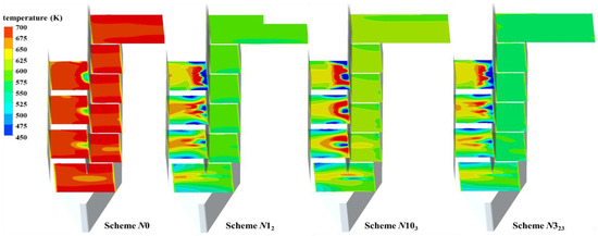
Figure 19.
Comparison of temperature in the furnace.
4. Conclusions
This work focuses on the flow field inside an SCL1000-13.5/450 grate boiler by means of a numerical simulation method. The simulated working condition complies with the operating instruction, which is verified by experimental measurement. In order to minimize inconsistencies of both velocity and temperature, spirally twisted tape inserts (STTIs) are installed in vertical flues of the grate furnace. Three kinds of arrangement schemes designed with the orthogonal experimental method are studied, including separate installation in chamber II (N12~N92), separate placement in chamber III (N13~N103), and simultaneous arrangement in both chambers II-III (N123~N923). According to the qualitative and quantitative analysis, the following conclusions can be reached:
- (1)
- Taking dispersion coefficients of velocity and temperature as indicators, STTIs should be arranged with a row spacing of 1.5 m and a column spacing of 2 m at an installation angle of 30° under the circumstance of separate installation in chamber II.
- (2)
- On the premise of exclusive utilization, the installation of STTI in chamber II is more beneficial for the uniformity of the flow field, which also exerts an active influence on the flow field of chamber III. Implementation of scheme N12 would bring down the average temperature of chamber III to 584.19 K.
- (3)
- According to comprehensive performance, the optimal combination scheme is N323, with STTIs arranged simultaneously in chamber III at the height of 22 m, 20.5 m and 19 m, located in sections of z = −4 m, z = 0 m and z = 4 m at an included angle of 60° to the width direction.
Author Contributions
Conceptualization, C.Y. and Z.J.; methodology, J.K.; software, X.C.; validation, X.C., C.Y. and Z.J.; formal analysis, Z.J.; investigation, C.Y.; resources, C.Y.; data curation, C.Y.; writing—original draft preparation, C.Y.; writing—review and editing, X.C.; visualization, J.Q.; supervision, J.Q.; project administration, Z.J.; funding acquisition, J.Q. All authors have read and agreed to the published version of the manuscript.
Funding
This research was funded by the National Natural Science Foundation of China through grant number 52175067 and 52176046 and State Key Laboratory for Clean Energy Utilization through grant number ZJUCEU2022022.
Data Availability Statement
The data presented in this study are available on request from the corresponding author.
Conflicts of Interest
Author Chen Yang was employed by the company China Ship Scientific Research Center. The remaining authors declare that the research was conducted in the absence of any commercial or financial relationships that could be construed as a potential conflict of interest.
References
- Indrawan, N.; Thapa, S.; Bhoi, P.R.; Huhnke, R.L.; Kumar, A. Electricity power generation from Co-gasification of municipal solid wastes and biomass: Generation and emission performance. Energy 2018, 162, 764–775. [Google Scholar] [CrossRef]
- Kanhar, A.; Chen, S.; Wang, F. Incineration Fly Ash and Its Treatment to Possible Utilization: A Review. Energies 2020, 13, 6681. [Google Scholar] [CrossRef]
- Emilio EG, P.; Fernández-Rodríguez, E.; Carrasco-Hernández, R.; Coria-Páez, A.L.; Gutiérrez-Galicia, F. A comparison assessment of landfill waste incineration and methane capture in the central region of Mexico. Waste Manag. Res. 2022, 40, 1785–1793. [Google Scholar] [CrossRef] [PubMed]
- Metolina, P.; Lopes, G.C. Numerical analysis of liquid-solid flow in tapered and cylindrical fluidized beds for wastewater treatment and biogas production. Energy Convers. Manag. 2019, 187, 447–458. [Google Scholar] [CrossRef]
- Saleh, A.R.; Sudarmanta, B.; Fansuri, H.; Muraza, O. Syngas production from municipal solid waste with a reduced tar yield by three-stages of air inlet to a downdraft gasifier. Fuel 2020, 263, 116509. [Google Scholar] [CrossRef]
- Sun, Y.; Qin, Z.; Tang, Y.T.; Huang, T.; Ding, S.; Ma, X. Techno-environmental-economic evaluation on municipal solid waste (MSW) to power/fuel by gasification-based and incineration-based routes. J. Environ. Chem. Eng. 2021, 9, 106108. [Google Scholar] [CrossRef]
- Pan, P.; Zhang, M.; Xu, G.; Chen, H.; Song, X.; Liu, T. Thermodynamic and Economic Analyses of a New Waste-to-Energy System Incorporated with a Biomass-Fired Power Plant. Energies 2020, 13, 4345. [Google Scholar] [CrossRef]
- Razmjoo, N.; Sefidari, H.; Strand, M. Measurements of temperature and gas composition within the burning bed of wed woody residues in a 4MW moving grate boiler. Fuel Process. Technol. 2016, 152, 438–445. [Google Scholar] [CrossRef]
- Liu, B.C.; Han, Z.Y.; Liang, X.Q. Dioxin emissions from municipal solid waste incineration in the context of waste classification policy. Atmos. Pollut. Res. 2023, 14, 101842. [Google Scholar] [CrossRef]
- Li, P.F.; Shimaoka, T. Recovery of Zn and Cu from municipal solid waste incineration fly ash by integrating ammonium leaching and ammonia removal. Waste Manag. 2024, 178, 115–125. [Google Scholar] [CrossRef]
- Ding, Z.Y.; Li, W.J.; Chen, Z.B.; Wang, L.; Huang, S.; Evrendilek, F.; Yang, C.; Cai, H.; Zhong, S.; Yang, Z.; et al. Microplastics as emerging contaminants in textile dyeing sludge: Their impacts on co-combustion/pyrolysis products, residual metals, and temperature dependency of emissions. J. Hazard. Mater. 2024, 466, 133465. [Google Scholar] [CrossRef] [PubMed]
- Kurniawan, T.A.; Liang, X.; O’Callaghan, E.; Goh, H.; Othman, M.H.D.; Avtar, R.; Kusworo, T.D. Transformation of Solid Waste Management in China: Moving Towards Sustainability Through Digitalization-Based Circular Economy. Sustainability 2022, 14, 2374. [Google Scholar] [CrossRef]
- Chen, S.S.; Huang, J.L.; Xiao, T.T.; Gao, J.; Bai, J.; Luo, W.; Dong, B. Carbon emissions under different domestic waste treatment modes induced by garbage classification: Case study in pilot communities in Shanghai. Sci. Total Environ. 2020, 717, 137193. [Google Scholar] [CrossRef] [PubMed]
- Zhao, F.; Bian, R.; Zhang, T.; Fang, X.; Chai, X.; Xin, M.; Li, W.; Sun, Y.; Yuan, L.; Chen, J.; et al. Characteristics of polychlorinated dibenzodioxins/dibenzofurans from a full-scale municipal solid waste (MSW) incinerator in China by MSW classification. Process Saf. Environ. Prot. 2022, 161, 50–57. [Google Scholar] [CrossRef]
- Gu, T.B.; Ma, W.C.; Berning, T.; Guo, Z.; Andersson, R.; Yin, C. Advanced simulation of a 750 t/d municipal solid waste grate boiler to better accommodate feedstock changes due to waste classification. Energy 2022, 254, 124338. [Google Scholar] [CrossRef]
- Fu, Z.; Zhang, S.H.; Li, X.P.; Shao, J.; Wang, K.; Chen, H. MSW oxy-enriched incineration technology applied in China: Combustion temperature, flue gas loss and economic considerations. Waste Manag. 2015, 38, 149–156. [Google Scholar] [CrossRef]
- Zhang, Y.; Du, X.; Yue, M.; Yan, M.; Shi, Y. Heat transfer and ash deposition performance of heat exchange surface in waste incineration flue gas. Int. J. Heat Mass Transf. 2020, 155, 119691. [Google Scholar] [CrossRef]
- Du, Y.F.; Ju, T.Y.; Meng, Y.; Lan, T.; Han, S.; Jiang, J. A review on municipal solid waste pyrolysis of different composition for gas production. Fuel Process. Technol. 2021, 224, 107026. [Google Scholar] [CrossRef]
- Liu, A.; Fan, R.; Liu, Q.; Xi, L.; Zeng, W. Numerical and Experimental Study on Combustion Characteristics of Micro-Gas Turbine Biogas Combustor. Energies 2022, 15, 8302. [Google Scholar] [CrossRef]
- Chang, J.H.; Oh, J.; Lee, H. Development of a roller hearth furnace simulation model and performance investigation. Int. J. Heat Mass Transf. 2020, 160, 120222. [Google Scholar] [CrossRef]
- Cardoso, J.; Silva, V.; Eusébio, D. Process optimization and robustness analysis of municipal solid waste gasification using air-carbon dioxide mixtures as gasifying agent. Int. J. Energy Res. 2019, 43, 4715–4728. [Google Scholar] [CrossRef]
- Shen, J.X.; Li, F.S.; Li, Z.H.; Wang, H.; Shen, Y.; Liu, Z. Numerical investigation of air-staged combustion to reduce NOx emissions from biodiesel combustion in industrial furnaces. J. Energy Inst. 2019, 92, 704–716. [Google Scholar] [CrossRef]
- Netzer, C.; Li, T.; Seidel, L.; Mauß, F.; Løvås, T. Stochastic Reactor-Based Fuel Bed Model for Grate Furnaces. Energy Fuels 2021, 34, 16599–16612. [Google Scholar] [CrossRef]
- Zeeshan, M.; Pande, R.R.; Bhale, P.V. A modeling study for the gasification of refuse-derived fuel as an alternative to waste disposal. Environ. Dev. Sustain. 2023, 26, 23985–24008. [Google Scholar] [CrossRef]
- Taki, M.; Rohani, A. Machine learning models for prediction the Higher Heating Value (HHV) of Municipal Solid Waste (MSW) for waste-to-energy evaluation. Case Stud. Therm. Eng. 2022, 31, 101823. [Google Scholar] [CrossRef]
- Vanierschot, M.; Hoang, Q.N.; Croymans, T.; Pittoors, R.; Van Caneghem, J. A CFD-based porous medium model for simulating municipal solid waste incineration grates: A sensitivity analysis. Fuel 2023, 345, 128221. [Google Scholar] [CrossRef]
- Wu, W.; Zhang, M.; Wang, Y.; Zhao, L.; Dong, H.; Zhang, J. Optimization of a pyrolysis furnace using multi-jet arrays through numerical and machine learning techniques. Int. J. Heat Mass Transf. 2023, 214, 124426. [Google Scholar] [CrossRef]
- Wei, G.; Zhang, H.; An, X.; Dianyu, E. Numerical investigation on the mutual interaction between heat transfer and non-spherical particle dynamics in the blast furnace raceway. Int. J. Heat Mass Transf. 2020, 153, 119577. [Google Scholar] [CrossRef]
- Wei, Y.H.; Kuang, M.; Zhu, Q.Y.; Ling, Z.; Ti, S.; Li, Z. Alleviating gas/particle flow deflection and asymmetric combustion in a 600 MWe supercritical down-fired boiler by expanding its furnace throat space. Appl. Therm. Eng. 2017, 123, 1201–1213. [Google Scholar] [CrossRef]
- Yang, Z.H.; Li, K.; Zeng, W.Z.; Li, B.; Liu, S. Design and analysis of a novel furnace throat for removing dust particles in flue gas emitted from copper smelting furnace by a computational method. Environ. Sci. Pollut. Res. 2019, 26, 27180–27197. [Google Scholar] [CrossRef]
- Chen, J.K.; Tang, J.; Xia, H.; Yu, W.; Qiao, J. Modelling the furnace temperature field of a municipal solid waste incinerator using the numerical simulation and the deep forest regression algorithm. Fuel 2023, 347, 128511. [Google Scholar] [CrossRef]
- Chen, X.J.; Yang, C.; Kong, J.X.; Wang, F.L.; Jin, Z.J.; Qian, J.Y. Steam-side heat transfer analysis in spirally corrugated tube for grate furnace superheater. Case Stud. Therm. Eng. 2023, 50, 103443. [Google Scholar] [CrossRef]
- Deshmukh, R.; Raibhole, V.N. Investigation of a natural convection heat transfer enhancement of a different shaped pin fin heat sink for different vertical fin spacing. Heat Mass Transf. 2023, 59, 2131–2148. [Google Scholar] [CrossRef]
- Liang, Y.M.; Liu, P.; Zheng, N.B.; Shan, F.; Liu, Z.; Liu, W. Numerical investigation of heat transfer and flow characteristics of laminar flow in a tube with center-tapered wavy-tape insert. Appl. Therm. Eng. 2019, 148, 557–567. [Google Scholar] [CrossRef]
- Kazerooni, R.B.; Bakhtiarpour, M.A.; Noghrehabadi, A. Experimental study of flow boiling heat transfer in horizontal rifled tube. Heat Mass Transf. 2023, 59, 477–487. [Google Scholar] [CrossRef]
- Ryu, C.; Shin, D.; Choi, S. Combined simulation of combustion and gas flow in a grate-type incinerator. J. Air Waste Manag. Assoc. 2002, 52, 189–197. [Google Scholar] [CrossRef][Green Version]
- Huo, Y.; Yu, Y.P.; Yang, D.; Zou, G.W.; Dong, H. Experimental study on the dynamic evolution of merged flame under the thermal effect of multiple fire sources in a shaft. Heat Mass Transf. 2023, 59, 2197–2211. [Google Scholar] [CrossRef]
- Zadravec, T.; Yin, C.G.; Kokalj, F.; Samec, N.; Rajh, B. The impacts of different profiles of the grate inlet conditions on freeboard CFD in a waste wood-fired grate boiler. Appl. Energy 2020, 268, 115055. [Google Scholar] [CrossRef]
- Rajh, B.; Yin, C.; Samec, N.; Hriberšek, M.; Zadravec, M. Advanced modelling and testing of a 13 MWth waste wood-fired grate boiler with recycled flue gas. Energy Convers. Manag. 2016, 125, 230–241. [Google Scholar] [CrossRef]


Disclaimer/Publisher’s Note: The statements, opinions and data contained in all publications are solely those of the individual author(s) and contributor(s) and not of MDPI and/or the editor(s). MDPI and/or the editor(s) disclaim responsibility for any injury to people or property resulting from any ideas, methods, instructions or products referred to in the content. |
© 2024 by the authors. Licensee MDPI, Basel, Switzerland. This article is an open access article distributed under the terms and conditions of the Creative Commons Attribution (CC BY) license (https://creativecommons.org/licenses/by/4.0/).