Abstract
The goal of increasing efficiency and durability of fuel cells can be achieved through optimal control of their operating conditions. In order to implement such controllers, accurate and computationally efficient fuel cell models must be developed. This work presents a hybrid (physics-based and data-driven), control-oriented model for approximating the output voltage of proton exchange membrane fuel cells (PEMFCs) while operating under dynamical conditions. First, a physics-based model, built from simplified electrochemical, membrane dynamics and mass conservation equations, is developed and validated through experimental data. Second, a data-driven, neural network (echo state network) is trained, fitted and tested with the same dataset. Then, the hybrid model is formed as a parallel structure, where the simplified physics-based model and the trained data-driven model are merged through an algorithm based on Gaussian radial basis functions. The merging algorithm compares the output of both single models and assigns weights for computing the prediction of the hybrid result. The proposed hybrid model structure is successfully trained, validated and tested with an experimental dataset originating from fuel cells within an automotive PEMFC stack. The hybrid model is assessed through the mean square error index, with the result of a low tracking error.
1. Introduction
The evidence of climate change induced by human activity has pushed the search for sustainable forms of production, storage and conversion of energy. Hydrogen has emerged as a promising energy carrier in a future low-carbon economy, and fuel cells are likely the ideal option for converting hydrogen’s chemical energy into electrical energy. Different types of fuel cells offer specific advantages for specific sectors. Low-temperature proton exchange membrane fuel cells (PEMFCs) have shown to be specially suitable to replace hydrocarbon-based engines in heavy duty vehicles. In order to achieve this goal, the durability and efficiency of PEM fuel cells must be improved. Some studies have set the durability goal in 25.000 h for these applications [1].
Fuel cells are complex devices that transform chemical energy into electricity through electrochemical reactions. Specifically, a low-temperature PEM fuel cell is fed with hydrogen in the anode side and oxygen (air) in the cathode side. The hydrogen undergoes an oxidation reaction, releasing electrons that travel through an external circuit to feed an electrical load. Positive hydrogen ions then travel through a membrane to the cathode side and join, through a reduction reaction, with the oxygen and the electrons returning from the external circuit. This is an exothermic process, with water as the main byproduct [2].
Applications of PEMFCs include their use in stationary implementations such as residential micro-combined cooling heating and power systems (CCHP) [3]. In this case, not only the electrical energy produced by the fuel cell is used but also the heat produced in the reactions is used for residential heating. Also, big advancements are being performed in the automotive industry to integrate PEM fuel cells in the powertrain of transportation vehicles [4].
The objective of extending PEMFCs’ useful lifetime and improve their efficiency is possible by applying proper control strategies. It has been proved that the integrity and performance of PEM fuel cells are highly dependant on their operating conditions. There exist relations between conditions, such as load profile or operating temperature, and the degradation of platinum in the cathode catalyst layer (CCL) [5]. Also, the corrosion of the carbon support in the catalyst layer can be explained through the values of fuel cell humidity and load profile [6]. Mathematical expressions for several degradation mechanisms, including dissolution and oxidation of platinum in the CCL, as a function of the operating humidity, voltage and temperature, have been proposed and validated [7]. Studies on PEMFC automotive applications have developed semi-empirical models that relates CCL durability to fuel cell conditions of operation [8].
Extending durability and decreasing degradation of PEM fuel cells are topics in which large research efforts are being invested. Health-aware control designs have been proposed also from the point of view of the energy management system installed in hybrid power electric vehicles, that is, vehicles where the power source alternates between a PEM fuel cell and a battery. This approach focuses on the control of the power delivered by the fuel cell and has given very promising results. Health-aware control through a reinforcement learning-based control is proposed in [9]. Also, a model predictive controller in conjunction with a machine learning-based model is proposed in [10] for decreasing a fuel cell hybrid electric bus.
In summary, improvements in fuel cell durability and efficiency depend on optimal control of the operating conditions and, for such control, accurate and computationally efficient models are required. Due to the complex and nonlinear interactions between their constitutive physical parameters, internal states and external operating conditions, fuel cells are challenging systems for modeling tasks.
Some models have proposed the combination of static and dynamic fuel cell behavior for prognosis purposes [11]. Also, in order to simplify the high non-linearity of fuel cell analytical expressions, there are linearized parameter-varying models [12]. PEMFC dynamics have also been modeled using equivalent electric circuits [13]. There has been extensive research on developing physics-based models of the PEMFC and its auxiliary systems, with several degrees of accuracy and computational cost [14].
In general, there is increasing interest in complementing models derived from the knowledge of underlying physical phenomena, with models built exclusively from data. The goal is to leverage strengths in the physic-based and data-driven modeling approaches, respectively. Hybrid architectures aim to model complex, nonlinear behaviors, systems with non- constant parameters or non-stationary processes. Hybrid models for complex nonlinear systems have been proposed in areas such as manufacturing [15]; the food industry [16]; the chemical/oil/gas industry [17,18,19]; and biological systems [20,21,22].
In research areas closer to fuel cell research, hybrid models are used for estimating the lifetime of lithium ion batteries by merging neural networks and Kalman filtering state estimation [23]. In this structure, the neural network forecasts future values of the observation variable (output measured variable), that is, the neural network replaces the observation equation. The function of the Kalman filter is to estimate the hidden state variables. In [24], a hybrid structure composed of a neural network and Kalman filter is presented to perform state estimation and forecasting.
The present work proposes a hybrid, control-oriented model to forecast the output voltage of a PEMFC operating under dynamical conditions. The goal of this paper is to fill the research gap in computationally efficient PEMFC models that is able to represent behaviors of fuel cells that are hard to forecast and that appear when the operating conditions vary dynamically. The most important contribution of this work is the design, implementation and validation of a hybrid modeling structure formed by three main components: a simplified physics-based model, an echo state network (ESN) and a merging algorithm based on Gaussian radial basis functions (GRBF). The novel features of the present work are detailed next:
- 1.
- The dataset used to train, test and validate the hybrid model comes from experiments where the operating conditions, and thus the profile of the output voltage, change dynamically, as opposed to the vast majority of datasets utilized in fuel cell modeling where the data come from static polarization curve experiments. Dynamical profiles of the operating conditions allow the showing of complex and hard-to-model behavior within the PEMFC.
- 2.
- The data-driven component of the hybrid structure is an ESN. As per the authors knowledge, this work represents the first implementation of an ESN for fuel cell modeling and voltage forecasting in a hybrid architecture.
- 3.
- A recursive GRBF is proposed for merging the contribution of each model. The GRBF recursively compares the similarity between the output of each model and the measured output of the fuel cell, assigns weights to each and computes the output of the hybrid structure.
The present paper is organized as follows. Section 2 describes the experimental setup and explains the most important features of the dataset. Section 3 presents the simplified physics-based model. Section 4 presents the data-driven model, and describes its fundamental parameters and the tuning procedure. Section 5 presents the hybrid structure and the merging approach. Section 6 shows and compares the results obtained from each model. Finally, conclusions and proposals for future research direction are presented in Section 7.
2. Experimental Setup and Data
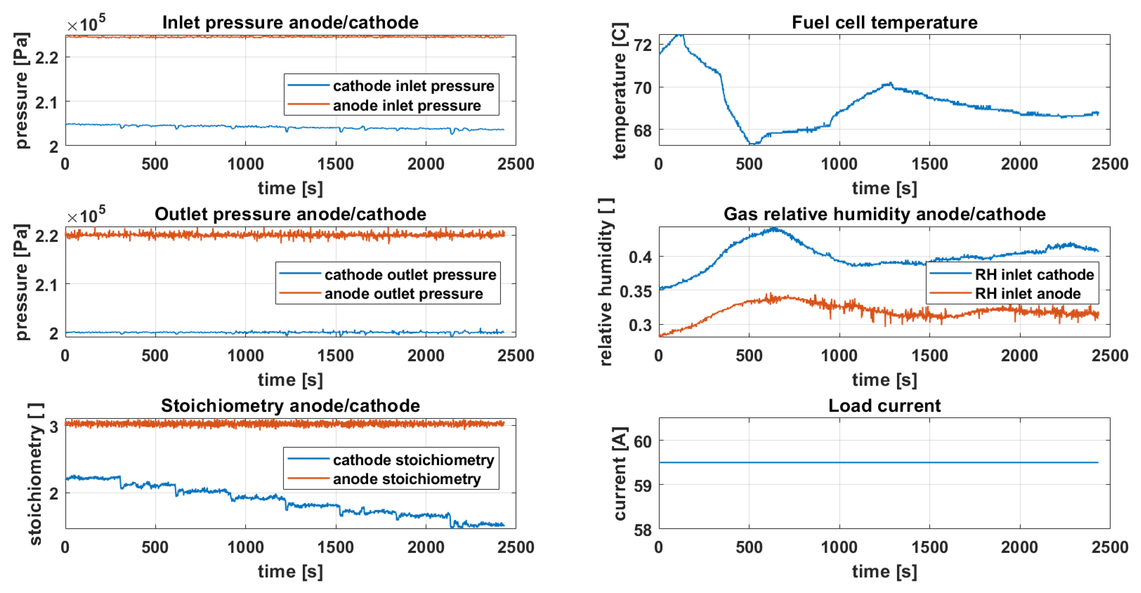
The dataset used to build, validate and test the hybrid model comes from experimental tests conducted on an automotive PEM fuel cell stack as part of the INN-BALANCE European research project [25]. The objective of the experimental tests was to analyze the effect of dynamic changes in the operating conditions on the voltage profile of the stack. The PEMFC stack was fed with pure hydrogen and air. A total of 12 operating conditions could be controlled: inlet pressure in the anode and cathode, outlet pressure in the anode and cathode, relative humidity, stoichiometry and flow of the inlet gases in the anode and cathode, temperature of the stack and load current. In each experiment, one operating condition was changed dynamically and the rest were kept constant. The dataset used for the present work corresponds to experiments in which the cathode stoichiometry is swept downward in regular steps while all the other operating conditions are set approximately constant. The cell voltage has been normalized to the value of the theoretical voltage at standard conditions, that is, 1.229 V; Figure 1.
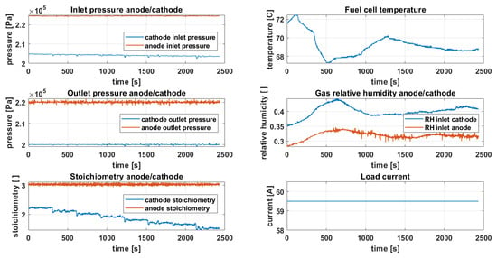
Figure 1.
Operating conditions.
A total of eight different conditions have been tested and are described in Table 1.

Table 1.
Table summarizing the several operating conditions tested.
The resulting output voltage is shown in Figure 2. The experiment shows highly nonlinear, hard-to-model behaviors of PEM fuel cells. As it has been shown by several studies, changing the cathode stoichiometry cause changes in the output voltage; in general, decreasing values of air stoichiometry result in decreasing values of voltage, and vice versa. This response has been studied mostly on static conditions through the analysis of polarization curves. However, as it can be seen in Figure 2, during dynamic operation and within certain regions of current, the output voltage does not follow exactly the decreasing profile of the stoichiometry. Instead, the voltage presents a recovery in some portions of the downward step.
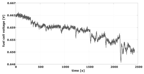
Figure 2.
Fuel cell output voltage.
The hypothetical explanation for this phenomenon is that, depending on the value of other fundamental operating conditions such as the temperature of the fuel cell, the relative humidity of the inlet gasses and load current, internal hidden states, which define cell voltage, change in a hard-to-model, nonlinear manner.
3. Physics-Based Model
3.1. Electrochemical Dynamics
The fuel cell voltage, , can be approximated by the subtraction a series of voltage losses from the theoretical Nernst potential [26],
The current density, , through the PEMFC depends on the external electrical load, and the fuel cell temperature, , is a state and an operating condition of the fuel cell, which can be set by the cell cooling system.
The cell voltage, Equation (1), has four specific expressions: Nernst voltage, , voltage loss due to activation overpotential, , voltage loss due to ohmic resistance, , and voltage loss due to the changes in concentration of the reactants in the catalyst layer, :
where is the exchange current density, is the ohmic cell resistance and is the limiting current, all of them time-varying parameters. In the case of the limiting current, it will be considered as a constant in the present work due to the region of operation where the fuel cell under study is being tested. The number of electrons obtained in the oxygen reduction reaction, n, and the charge transfer coefficient, , are fixed parameters. R is the ideal gas constant and F is the Faraday constant.
The Nernst voltage depends on the temperature of the fuel cell and the partial pressure of hydrogen and oxygen [27],
where corresponds to a reference temperature of 298.15 K. is the cathode partial pressure (oxygen) and is the anode partial pressure (hydrogen).
The exchange current density is a function of the operating temperature and the partial pressure of oxygen:
, with units of , and , with units of , are two parameters that represent the amount of platinum in the catalyst layer and its active area, respectively. The combination of these two parameters is called the electrochemical active surface area (ECSA) of the fuel cell. There is a fixed reference exchange current density, , specific for each catalyst material. is the Gibbs activation energy [28]. The exchange current density in the anode of a PEMFC is three-to-four orders of magnitude larger than that of its cathode. This means that the voltage losses due to activation energy (the process where the exchange current density intervenes) are negligible in the anode [26]. Based on this widely accepted result, only the activation losses in the cathode are considered in the simplified model presented in this work.
The ohmic cell resistance is approximated to the membrane resistance in this work, and the ohmic losses of other regions of the fuel cell (i.e., bipolar plates) are neglected. Thus, the ohmic cell resistance (or ohmic membrane resistance) can be computed by Equations (7) and (8) per, [29]:
where is the constant membrane thickness, and , the membrane conductivity, is computed by:
The coefficient is constant and is related to the water content of the membrane, , through:
3.2. Gas Channel Dynamics
A mass balance analysis is performed to estimate the partial pressure of oxygen in the CCL :
Equation (9) represents the relation between the ratio of partial pressure of oxygen to total outlet air pressure (whose value is provided in the dataset) and the ratio of oxygen molar flow to the sum of molar flows of the components of air in the cathode, that is, molar flow of oxygen, , molar flow of nitrogen, , and molar flow of water vapor, . These flows are defined in Equations (10), (11) and (12), respectively:
The added subscripts “in” and “ORR” signal whether the source of corresponding flow is the cathode inlet or the oxygen reduction reaction. In order to compute the inlet molar flow of vapor, the temperature and relative humidity of the inlet air, provided in the dataset, are used.
The inlet vapor saturation pressure, , is computed through Equation (13). is the inlet air temperature, is the inlet air relative humidity and is a fitting coefficient (Table 2). Once the inlet vapor pressure, , is computed, Equation (14), the partial pressure corresponding to the dry inlet air, , and the molar mass of the dry inlet air, , being the molar mass of x, are computed through Equations (15) and (16), respectively:
The molar flow of vapor entering the cathode, , can then be computed using the humidity ratio, Equation (17). This is performed in Equations (18)–(20):
The vapor molar flow due to the ORR is computed by Equation (21):
In Equation (22), the mass portion of oxygen contained in dry air is represented by . The inlet and consumed molar flows of oxygen are:
The proposed development for computation of has an estimation error of around 10% for the operating range of the tested fuel cell [30]. This means that the computation of the Nernst voltage, based on Equation (5), would present an estimation error of less than 1%. Table 2 shows the values of the parameters and constants utilized in Equations (9)–(24).
3.3. Membrane Dynamics
The membrane model aims to describe the water content in the membrane. This value is used to compute the membrane ohmic resistance, . The membrane average water content, , is calculated averaging the water activities in the anode, , and cathode, , which can be calculated from the approximated vapor partial pressure, Equations (25)–(27), per [29]:
for and where or are calculated through Equation (13).
The computed is then introduced in Equation (8) to approximate the membrane ohmic resistance.
4. Data-Driven Model
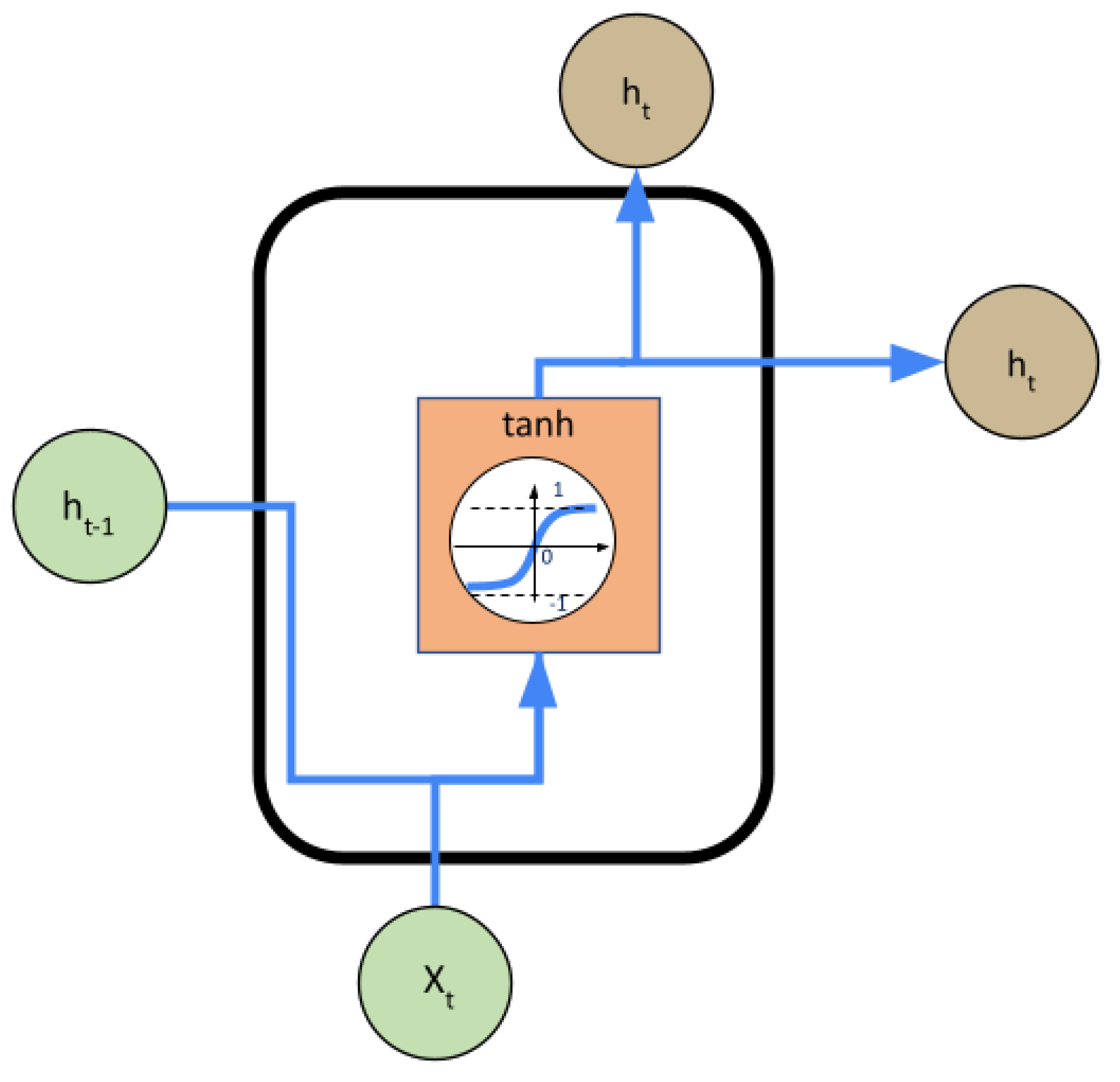
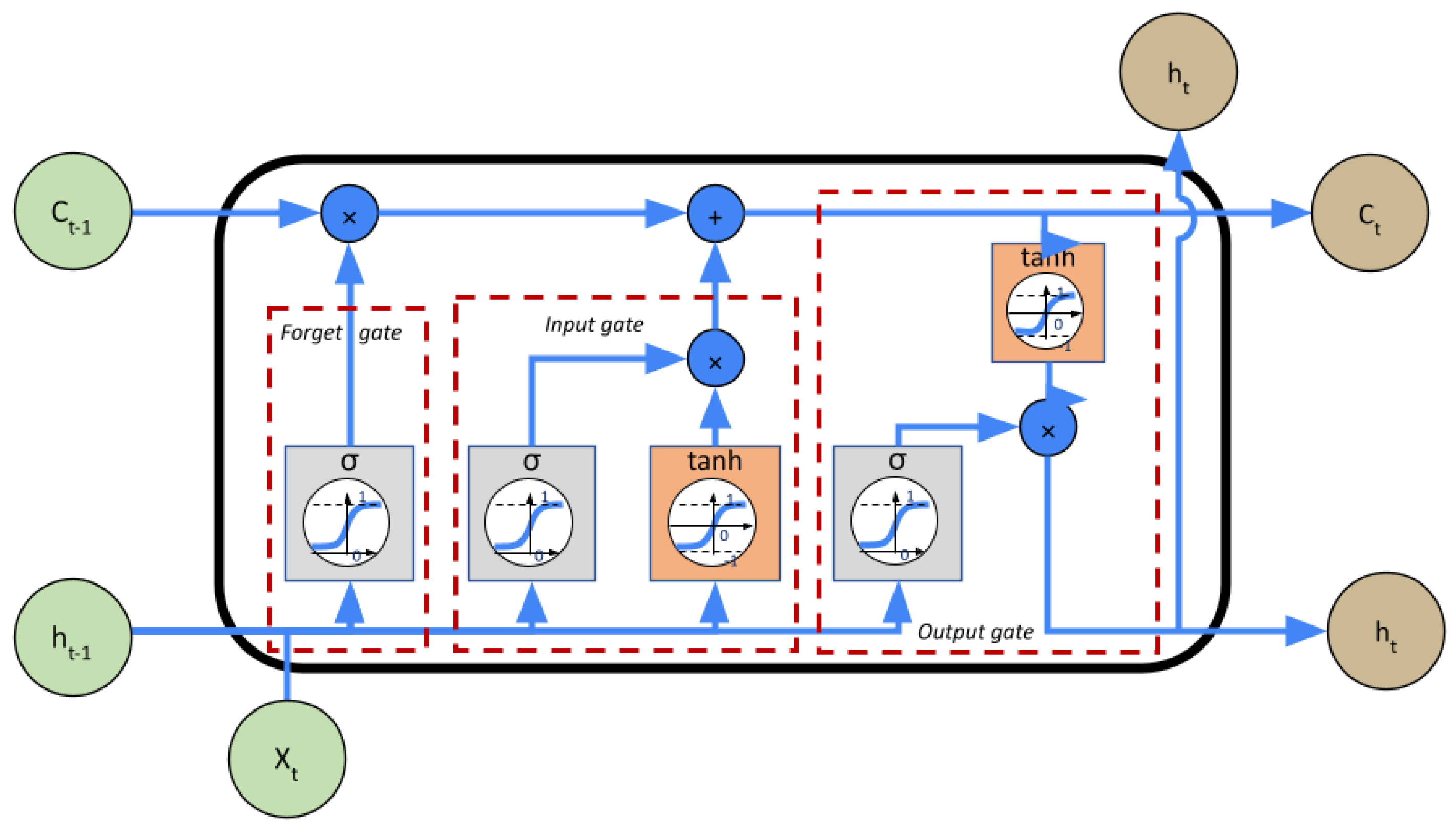
In order to complete the information provided by the physics-based model, a data-driven model was used in parallel. The interest of this structure is to adjust the predictions made by the physical model by using the data-driven model to use historical data and capture more complex dynamics that are difficult to represent. The data-driven model is based exclusively on historical data. The computation is made by an IA algorithm. The challenges are finding the best tool to catch the dynamics of the variable evolution with a low computational effort, the setting of the algorithm parameters and the quality of the data available for the training step. One of the best-known data-driven algorithms dedicated to the forecasting task is the recurrent neural network (RNN). Indeed, they allow the capturing of temporal information at different scales, which make them suitable for this forecasting task. However, classical optimization methods such as back-propagation do not provide good performances and can lead to vanishing gradient problems, where the derivative calculated for some network weights becomes so small that no change is made between epochs [31,32]. Another possibility is to use long short-term memory (LSTM) [33] or gated recurrent unit (GRU) [34] networks. The architecture of these networks helps to preserve the error that can be back-propagated through time and layers. LSTM cells are composed of three gates, which are input, output and forget gates. They allow the keeping or erasing of the information stored in the memory. The input gate represents new information added to the cell state, the forget gate decides what information is to be stored or deleted, while the output gate corresponds to the output of the LSTM. The principle of GRU cells is very similar to that of LSTM. The input and forget gates are simplified to an update gate, and a reset gate is used to control how much past information is to be forgotten. Since the architecture of GRU cells is simpler than that of LSTM, they are more computationally efficient. According to the empirical study in [35], GRU cells are more attractive when the sequence is long and the datasets are small. In other scenarios, the performance losses compared with LSTM are more serious. Figure 3, Figure 4 and Figure 5 present the principle of the three cells.
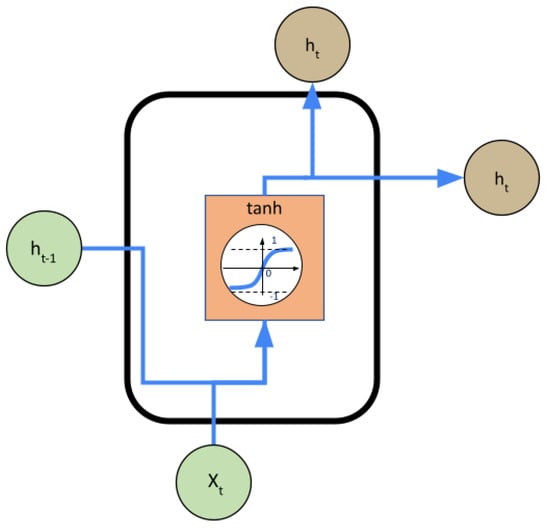
Figure 3.
Structure of an RNN.

Figure 4.
Structure of a GRU.
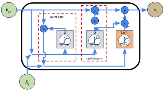
Figure 5.
Structure of a LSTM.
Even though there have been large improvements in RNN architectures, training these neural networks using back-propagation through time consumes high computational resources. To compensate for this limitation, reservoir computing (RC) uses an approach that is significantly different. The RC principle is to map one or more input signals into a high-dimensional computational space containing abundant dynamic transient states (called a reservoir). For this, the reservoir weights are fixed and only a readout is trained. It has been developed independently by Jaeger and Maas in the form of echo state networks (ESNs) [32] and liquid state machines (LSMs) [36], respectively, in the early 2000s. In [37], a review of main reservoirs and readout training methods is proposed. Although the principle of the RC approaches is the same, differences can be found in the ways of initializing the reservoir and training the weights in the readout.
The data-driven model developed in this paper is based on the use of echo state networks. They have been widely used in several areas such as gesture recognition [38], motor control [39] and fuel cell remaining useful life rediction [40]. In addition, ESNs are easier to implement and tune than LSMs [37], which makes them interesting for embedded applications.
4.1. Echo State Networks
According to the work of Jaeger in [32], ESNs can be represented by three layers. First of all, the information is received by neurons in the input layer. Then, the information is propagated in a high-dimensional space named reservoir composed of a high number of neurons whose weights are fixed during the initialization. The last step is the transmission of the information from the reservoir to an output layer to read the results. Because the weights of the input and recurrent connections are fixed during the generation of the reservoir, only the output weights are trained through linear regression. This feature reduces the complexity of the network and its computation time compared with the usual methods (i.e., LSTM and GRU). Therefore, ESNs are able to process complex non-linear tasks using a simple structure.
4.1.1. Equations
First of all, for a better understanding of the equations below, the terminology is fixed. In this study, a discrete-time echo state network with K input units (i.e., features), N reservoir-internal units and L output units is considered. In addition, the discrete time is represented by , where T is the number of data points in the training database.
The input weights, W, are collected in a matrix of size K. The activation of the input neurons at time “n” is represented by the input vector: .
The reservoir weights, W, are collected in a matrix of size N. The activation of the reservoir neurons at time “n” is represented by the reservoir state vector: .
The output weights, W, are collected in a matrix of size (K + N + L). The activation of the output neurons at time “n” is represented by the output vector: .
For specific applications, an optional feedback weight matrix, W, of size L can be added between the output weight matrix and the reservoir.
The reservoir activation states are calculated using Equation (28) described below:
where f and n represent, respectively, the activation function of the neurons and the time step. In tasks where no output feedback is required (i.e., W is null), the activation of output neurons can be calculated using the result of Equation (29) presented below:
where is the activation function for the output neurons (generally identity) and is the concatenation of with .
The output weights are calculated by solving the linear equation system described below:
where X represents all produced by presenting the reservoir with u(n), and represents all .
4.1.2. Parameters
Besides their simplicity of use and optimization, ESNs come with a larger number of parameters to set: spectral radius, connectivity, leaky rate, amount of neurons and scaling factor.
Spectral radius: the spectral radius is used to set the intensity at which past states affect current states. The higher the value is, the more the past states will be reflected. Mathematically, it corresponds to the maximum eigenvalue of the reservoir matrix. It is determined during the initialization of the reservoir, where the matrix weight is generated randomly. In order to let the user control this parameter, a general solution is to normalize the matrix by dividing the matrix by its spectral radius value (range scaling). Another way is to divide the matrix by its Euclidean norm (norm scaling). In both cases, the normalized matrices are then multiplied by the desired value. It is recommended to have a spectral radius value of less than 1 in order to respect the echo state property (ESP), which implies that the initial conditions should gradually disappear with time, i.e., the state of the reservoir should depend only on the input signal and not on the initial conditions existing before this input. According to the study carried out in [41], the ANOVA method has been applied to ESNs, and results show that the spectral radius and the number of neurons are the most important parameters to define.
To take this limitation into account, in [42], the authors proposed to use Glorot distribution (also named Xavier distribution) [43], where the weights are directly initialized to follow a normal, truncated normal or uniform distribution depending on the number of inputs and outputs. This method eliminates the need to normalize weights using the spectral radius, thus reducing the number of parameters to be used. For normal and truncated normal distributions, , the standard deviation () is calculated as shown in Equation (32)
For a uniform distribution, , the bounds are determined as shown in Equation (33):
Leaky rate: the second parameter is the leaky rate, , which allows the controlling of the dynamics of neurons (also named leaky integrator neurons). The leaky value is in the interval [0, 1] and it represents the importance given to previous states of the reservoir to the calculation of the current state. A high leakage rate signifies that previous states have a low impact on current outputs. To integrate the leakage, it is necessary to modify the calculation of neurons presented in Equation (28) by Equation (34) shown below:
Connectivity: the third parameter is the connectivity (c), which represents a percentage of non-zero weights in the reservoir matrix. Adding zeros within the matrix allows the increasing of individual dynamics by decoupling into sub-networks. According to Lukoševičius in [44], the impact of connectivity on the results is relatively small. However, a sparsely connected reservoir improves computation times due to the fact that reservoirs are updated faster.
Neurons: in opposition to classical recurrent neural networks (RNN, LSTM, GRU), ESN reservoirs have the capacity to process a large number of neurons. This number can vary from a dozen to several thousand. Indeed the weights being fixed allows the simplification of computation times because the problem is transformed into a simple linear regression.
Scaling factor: the scaling factor represents the interval in which the input and feedback weights of the network will be fixed during initialization. For a normal distribution, this value is characterized by its standard deviation, and for a uniform distribution by its interval [−a, a]. Typically, echo state networks are used with hyperbolic tangent activation function, and scaling factors are in the interval [−1, 1] or a standard deviation of 0.5. Indeed, the closer the weights are to 0, the more linear the output will be because the hyperbolic tangent function is almost linear around 0.
4.1.3. Reservoir Combination
In order to cope with the increase in the number of parameters to be regulated, some architectures combining several reservoirs have been developed. The first combination is the use of bidirectional reservoirs. In order to increase the number of detectable dynamics in a sequence, a solution is to double the number of reservoirs. This allows learning input sequences in both chronological and reverse directions and thus gives the same importance to the weights situated at the beginning and end of sequences. In [45], Bianchi used a neural network composed of a bidirectional ESN (BiESN) and some feed-forward layers to classify time series. Bidirectionality can be used with all types of RNN approaches; however, due to the computation times, they are not often applied. The second combination is named a “multi-reservoir ESN” (MR ESN) and consists in using several small tanks instead of a large one. The tanks can be combined in series and/or in parallel, which makes it possible to use several configurations at the same time and thus avoid having a phase dedicated to the optimization of the reservoir parameters. In [46], Sun presents the main existing architectures combining several ESNs, and, in [47], a multi-reservoir bidirectional ESN (MR-BiESN) is used to forecast the voltage of a PEMFC in a static operating condition.
4.2. Data-Driven Model Designed
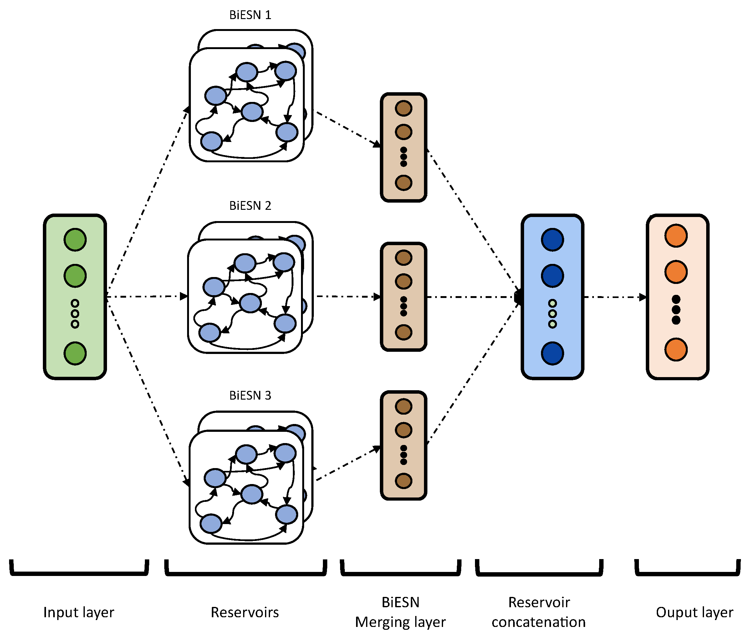
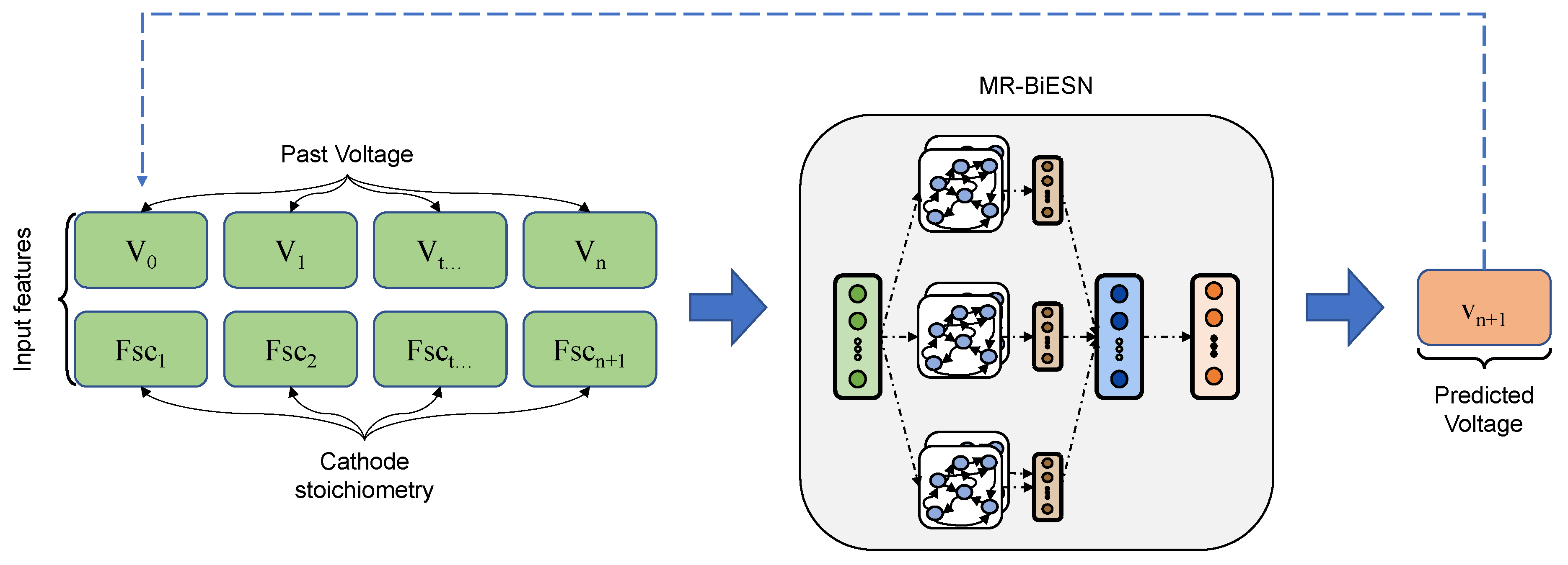
The main objective of the designed approach is to predict the future voltage of a PEMFC using past voltage and current. In order to reduce the computation time and also the training time (including the time needed to find the right combination of parameters), the use of a MR-BiESN seems to be a relevant choice. Indeed, as explained in the previous section, setting the parameter values to obtain good results needs both time and skills, as it is carried out by a trial and error approach or by an optimization tool. Furthermore, in the case of multiple dynamics to catch, the final set is a compromise to obtain the dominant one. An alternative is the use of multiple tanks, in parallel or in series, instead of a single large one. The parameters of the several subtanks are sorted in the usual range of values: the neuron dynamics of the relevant subtank are amplified and the dynamics of the irrelevant ones are extinguished during the training of the ESN. In the designed model, three bidirectional reservoirs are used in parallel. The parallel organization allows detection of the different dynamics contained in the data. Each reservoir is set to detect a type of dynamics (low, medium or fast). The data-driven architecture is presented in Figure 6 and selected parameters are described below and summarized in Table 3.

Figure 6.
Architecture of the designed data-driven model.

Table 3.
Table summarizing the parameters retained to design the data-driven model.
The dynamics of each reservoir are represented by a parametrization of the spectral radius and the leakage rate more or less largely according to the desired dynamics. In this study, the retained values for both parameters are 0.1, 0.5 and 0.9 (extreme and average values). The connectivity remains constant at 10%, which is a default value, and the number of neurons is fixed at 100. The input and reservoir weights are initialized using a Glorot uniform distribution. The advantage is that it directly takes into account the number of inputs and outputs and avoids having to search for a good value to bound the uniform distribution.
Inputs of the network are sequences representing the past voltage and cathode stoichiometry set by the user. An important parameter to define is the length of the sequence to be used, indeed, a too-short sequence cannot use the information of the past and a too-long sequence increases the complexity and the computing time. In this study, it has been chosen to train the network using the two last minutes with a sampling of 1 Hz. An important assumption is that, in order to predict the voltage at time t + 1, it is assumed that the user-defined cathode stoichiometry at time t + 1 is known. In a system, depending on the sampling frequency, this value can be estimated close to the last known value. This ensures that there is a shift in the learning sequences, as shown in Figure 7.
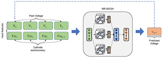
Figure 7.
Scheme representing the functioning of the data-driven model.
To improve performances and reduce optimization complexity, each feature has been normalized in the range [0, 1]. The activation function used in all reservoirs is the hyperbolic tangent (tanh), which is the default function for ESN. The selected optimization algorithm is the one presented in [48], entitled AdamW. The authors demonstrated that it is more interesting to decouple the weight decay parameter with the Adam optimizer in order to facilitate the search for parameters and also to obtain better results. The weight decay is a regularization hyper-parameter used to improve the generalization of models by avoiding over-fitting. The selected learning rate and weight decay are, respectively, 0.0012 and 0.001. During the training, the two parameters are scheduled to follow an exponential decay, with a decay rate of 0.95 for each 10 epochs. It has been shown empirically that the learning rate decay improves generalization and helps the optimization to reach a global optimum. Since the weight decay is decoupled, it is necessary to apply the same scheduling.
5. Hybrid Model
The proposed solution is to overcome the limitations of both the physics-based and the data-driven models, and to take advantage of the hybrid model’s capabilities to merge both models in a parallel structure. The hybrid model is formed by three main components: the physic-based model, the data-driven model and the merging function, Figure 8.
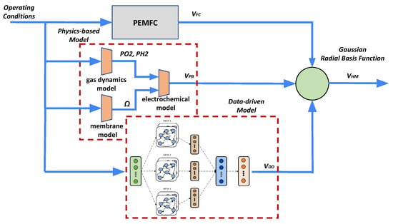
Figure 8.
Proposed hybrid model formed by a simplified physics-based model and a neural network.
The chosen hybridization method is through a radial basis function (RBF). RBFs are specific type of functions that deliver an output depending on the absolute difference between the input and a central parameter. RBFs have been successfully utilized as activation functions in neural networks for modeling and control of highly nonlinear systems such as biomass boilers [49], unmanned aerial vehicles [50] and new generation nuclear power plants [51].
Merging Function
The merging of models is based on a similarity function, the Gaussian radial basis function. This function measures the distance between measured (real) fuel cell voltage and the voltage approximated by the model, and assigns a weight, in the range to the voltage approximation at each sampling time:
for
where is the number of past samples that are taken into account to compute the weight of the approximation, is a tuning parameter related to the confidence of the model, k is the current sampling time, is the output voltage of the model (either data-driven or physics-based) and is the measured fuel cell voltage.
Then, the weights of each model are averaged for computing the contribution of each model to the prediction:
for
where is the averaged weight of each model, either data-driven (dd) or physics-based (pb), v is the voltage approximation of each model and is the prediction horizon.
6. Results and Discussion
6.1. Physics-Based Model
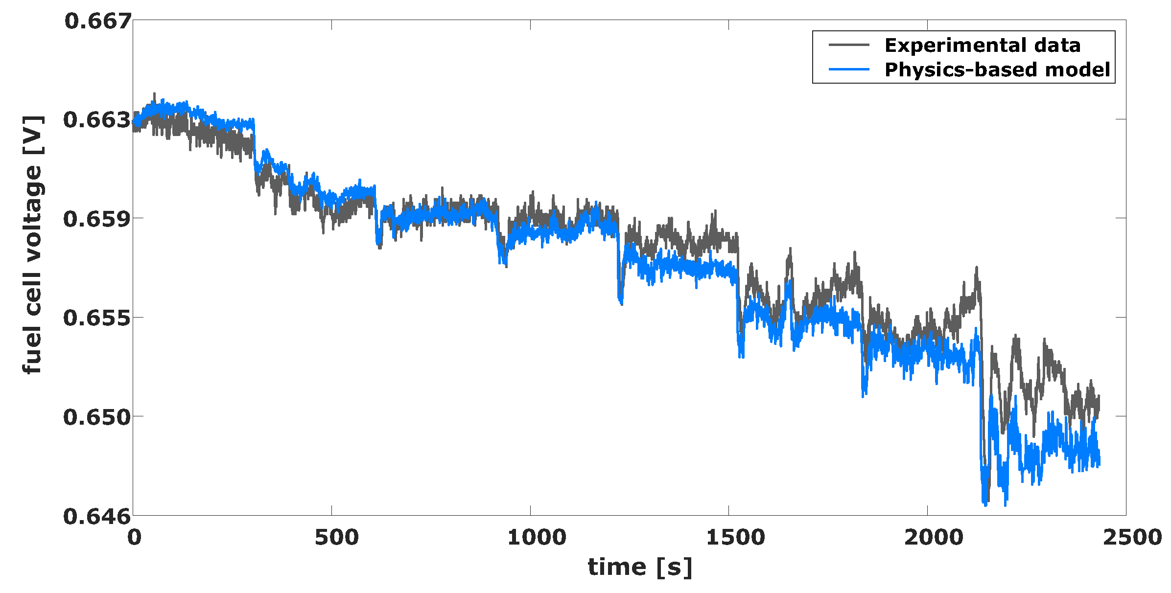
Figure 9 presents the results of the physics-based model. It can be seen that, even though the difference between the real and modeled voltage is in the range of fewer than ten millivolts, the model fails in following the trends and short-term dynamics of the voltage signal.
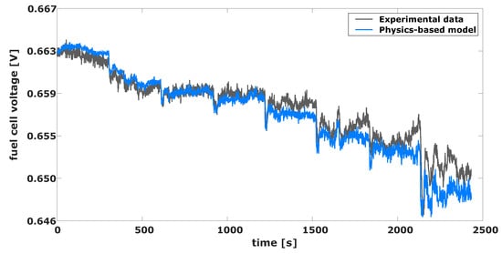
Figure 9.
Real voltage and physics-based model predicted voltage.
The difference in the trends at some sampling times can be explained by the simplifications and approximations carried out in the construction of the physics-based model. These include: overlooking the effect of several water dynamics that take place in the cathode catalyst layer, the approximations carried out in the equations that calculate the partial pressure of oxygen and hydrogen in the gas channels, the assumption that the fitting parameters are time-invariant and, in general, the fact that the model has been fitted to quasi-static operating point in the PEMFC (the polarization curve). The mean square error (MSE) of the model is shown in Table 4.

Table 4.
Mean square error of the different models at each phase of the cycle.
6.2. Data-Driven Model
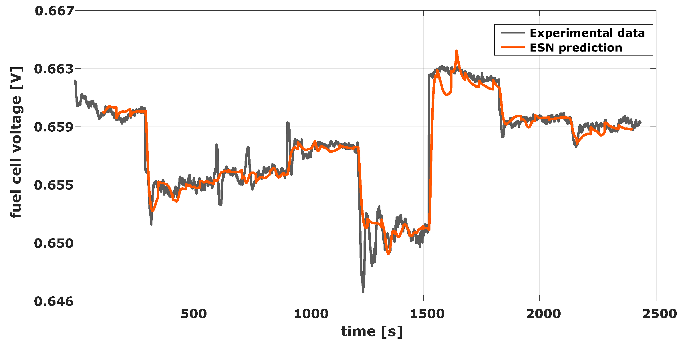
Regarding the date-driven model, it was trained using the data presented in Section 2. The objective of the proposed approach is to predict the next 60 s from the last 120 s. For that purpose, a new signal is constructed from the training data, in which the order of the tested conditions has been changed. The interest in reconstructing the signal is that it allows the measurement of the performance of the network during the transitions between two conditions. Moreover, to ensure that the model is able to generalize to intermediate conditions, conditions 2 and 5 presented in Table 3 have been removed from the training base and are used to test the model. This new reconstructed signal and the prediction results are presented in Figure 10.
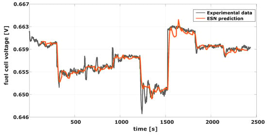
Figure 10.
Real voltage and physics-based model predicted voltage. Conditions presented in Table 1 have been shuffled in the order: [1, 6, 5, 4, 7, 0, 2, 3].
The results show that the data-driven method is able to capture the voltage evolution trends correctly while suppressing the noise observable during the signal measurement. The total MSE obtained is analyzed in Table 4. Furthermore, the generalization condition is met as the model correctly predicts conditions 2 and 5 (600–900 s and 1800–2100 s) that were not learned.
6.3. Hybrid Model
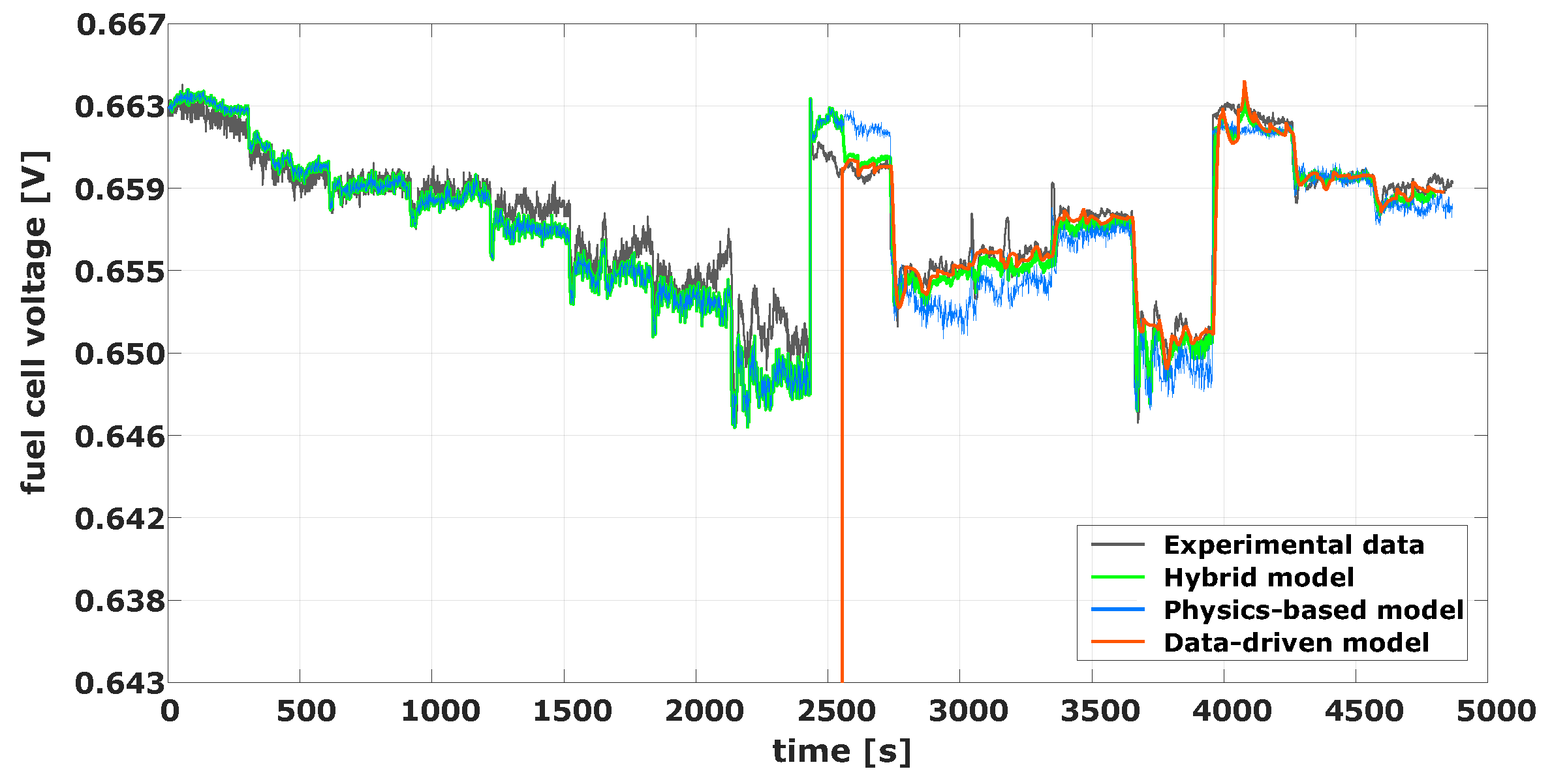
A new voltage profile is constructed by concatenating the experimentally measured voltage and the shuffled voltage signal used for testing the data-driven model. This concatenated signal represents a full cycle for the hybrid model, Figure 11. In the first phase (from s to s), during which the ESN is being trained, the data-driven model does not provide any valid voltage forecast and the voltage approximation is carried out exclusively by the physics-based model. Then, in the second phase, once the neural network has been trained, its forecast can be incorporated into the hybrid model and combined with the physics-based model. The discrimination and weighting of both models is carried out by the merging algorithm.
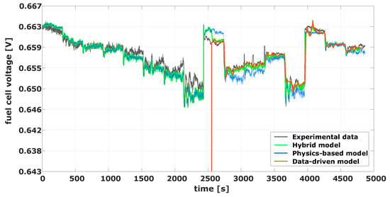
Figure 11.
Cell voltage and model voltage approximation.
It is expected that the two phases shown in Figure 11, which correspond to the training and prediction period of the ESN, occur periodically during the fuel cell lifetime. This is due to the fact that, when facing completely new operating conditions or when the internal parameters of the fuel cell suffer large variations due to degradation (i.e., aging), the ESN needs to be re-trained.
The modeling error of the three models is shown in Table 4. The MSE during each phase and the total MSE is calculated. It can be seen that, during the prediction phase, when both models contribute to approximate the output of the real fuel cell, the proposed hybridization achieves a lower modeling MSE than each of the models separately. The total MSE takes into account the whole cycle (training and prediction).
The proposed hybrid model has a number of advantages that can be summarized as follows:
- 1.
- The physics-based part of the hybrid model has been constructed from simplifications of the main internal dynamics of the fuel cell. This results in a fewer number of parameters needed to be fitted in comparison with more complex accurate models. This allows a time-efficient model construction process.
- 2.
- The chosen data-driven model, an ESN, is an efficient neural network architecture with fast training times and simpler training algorithms than other neural networks. This results in a less time-consuming fitting process.
- 3.
- Due to the previous characteristic, the data-driven part of the hybrid model can be re-trained online, when the deviation between the system and the model is deemed too large. This would be nearly impossible with more complex architectures such as LSTM networks. The capacity to be re-trained on line is an enormous advantage with modeling systems whose parameters vary with time or suffer changes due to degradation, as is the case with important parameters in the PEM fuel cells (i.e., the amount of platinum in the catalyst layer).
- 4.
- By incorporating totally independent models in parallel, the hybrid structure is able to maintain a good approximation of the voltage during the full cycle of the fuel cell. Also, in case of failure of one the models, the hybrid model can still track the voltage with acceptable accuracy.
This model is meant for use in model-based controllers, such as the model predictive control (MPC). In an MPC (or any other optimization-based control strategy), a large amount of computation time is consumed at each sampling instant to solve the optimization problem. Thus, the time portion of the control algorithm dedicated to approximate values of the system, that is, the model embedded in the controller, must be fast enough in order to lessen the computation burden. The model is also suitable for prognosis and forecast. In this application, the future evolution of fuel cell voltage can be approximated if future values of the operating conditions are known.
It is worth mentioning that one disadvantage of the chosen data-driven architectures is the need to set a series of fundamental parameters, whose setting is a rather iterative and heuristic process. These parameters define the performance of the ESN and when not set properly can lead to large deviations between model and system.
7. Conclusions
Fuel cells are promising energy conversion devices in a future hydrogen-based economy. However, issues such as efficiency and durability must be addressed, and the way of addressing them is by optimal the control of fuel cell operating conditions. The performance of such control depends largely on efficient and accurate models. This paper has proposed and tested a novel hybrid, data-driven/physics-based model for approximating fuel cell output voltage. The two models are merged through a recursive Gaussian radial basis function. The hybrid model has been trained, validated and tested with an experimental dataset, with dynamical profiles in operating conditions.
The main contributions of the present work are the presentation of a simplified physics-based model with a reduced number of fitting parameters, and the utilization of an ESN, with its simple training process, as the data-driven function approximator, and the proposed merging algorithm, which takes into account the error between both models to deliver an output that improves the approximation made by each model alone.
The future research directions will be to focus on the implementation of the hybrid architecture as the embedded fuel cell model of a model-based control strategy. Also, it is interesting to explore the use of the model as a prediction function in a hidden state estimator (or observer), such as a Kalman or particle filter. This application would allow for the computation of internal, not easily measurable, PEM fuel cell variables, which is a major issue in fuel cell research.
Author Contributions
Conceptualization, J.A.A.; Methodology, J.A.A. and D.C. (Damien Chanal); Investigation, J.A.A. and D.C. (Damien Chanal); Data curation, D.C. (Damien Chanal); Writing—original draft, J.A.A. and D.C. (Damien Chanal); Writing—review & editing, J.A.A. and D.C. (Damien Chanal); Supervision, D.C. (Didier Chamagne), N.Y.S., M.-C.P., A.H. and J.A.-C. All authors have read and agreed to the published version of the manuscript.
Funding
This research was funded by: Project MDM-2016-0656 and the program “ESF Investing in your future”, grant number BES-2017-082441, funded by MCIN/AEI /10.13039/501100011033. The European Union Fuel Cells and Hydrogen 2 Joint Undertaking through project INN-BALANCE, grant number 735969, and project RUBY, grant number 875047, website: https://www.rubyproject.eu (accessed on 1 December 2023). The contract “GEPEVE: Gestión predictiva de energía para eficiencia energética en vehículos eléctricos con control de crucero adaptativo” of the Movilidad 2030 project of the 2020 Misiones CDTI program. The Consolidated Research Group RAIG (2021 SGR 00510) of the Departament de Recerca i Universitats de la Generalitat de Catalunya. The doctoral school EIPHI, contract ANR-17-EURE-0002. The Region Bourgogne Franche-Comté, France. The APC was funded by the Consejo Superior de Investigaciones Científicas (CSIC), Spain.
Data Availability Statement
Data is contained within the article.
Conflicts of Interest
The authors declare no conflicts of interest.
References
- U.S. Department of Energy, Fuel Cell Technologies Office. Multi-Year Research, Development, and Demonstration Plan. 2014. Available online: www.energy.gov/eere/fuelcells/downloads/hydrogen-and-fuel-cell-technologies-office-multi-year-research-development (accessed on 2 July 2023).
- Agyekum, E.B.; Ampah, J.D.; Wilberforce, T.; Afrane, S.; Nutakor, C. Research Progress, Trends, and Current State of Development on PEMFC-New Insights from a Bibliometric Analysis and Characteristics of Two Decades of Research Output. Membranes 2022, 12, 1103. [Google Scholar] [CrossRef]
- Chen, X.; Gong, G.; Wan, Z.; Luo, L.; Wan, J. Performance analysis of 5Â kW PEMFC-based residential micro-CCHP with absorption chiller. Int. J. Hydrogen Energy 2015, 40, 10647–10657. [Google Scholar] [CrossRef]
- Olabi, A.G.; Wilberforce, T.; Abdelkareem, M.A. Fuel cell application in the automotive industry and future perspective. Energy 2021, 214, 118955. [Google Scholar] [CrossRef]
- Darling, R.; Meyers, J. Kinetic Model of Platinum Dissolution in PEMFCs. J. Electrochem. Soc. 2003, 150, A1523–A1527. [Google Scholar] [CrossRef]
- Pandy, A.; Yang, Z.; Gummall, M.; Atrazhev, V.; Kuzminyh, N.Y.; Sultanov, V.; Burlatskyb, S. A Carbon Corrosion Model to Evaluate the Effect of Steady State and Transient Operation of a Polymer Electrolyte Membrane Fuel Cell. J. Electrochem. Soc. 2013, 160, F972–F979. [Google Scholar] [CrossRef]
- Schneider, P.; Sadeler, C.; Scherzer, A.; Zamel, N.; Gerteisen, D. Fast and Reliable State-of-Health Model of a PEM Cathode Catalyst Layer. J. Electrochem. Soc. 2019, 166, F322–F333. [Google Scholar] [CrossRef]
- Kneer, A.; Wagner, N. A Semi-Empirical Catalyst Degradation Model Based on Voltage Cycling under Automotive Operating Conditions in PEM Fuel Cells. J. Electrochem. Soc. 2019, 166, F120–F127. [Google Scholar] [CrossRef]
- Jia, C.; Li, K.; He, H.; Zhou, J.; Li, J.; Wei, Z. Health-aware energy management strategy for fuel cell hybrid bus considering air-conditioning control based on TD3 algorithm. Energy 2023, 283, 128462. [Google Scholar] [CrossRef]
- Jia, C.; He, H.; Zhou, J.; Li, J.; Wei, Z.; Li, K. Learning-based model predictive energy management for fuel cell hybrid electric bus with health-aware control. Energy 2024, 355, 122228. [Google Scholar] [CrossRef]
- Lechartier, E.; Laffly, E.; Péra, M.C.; Gouriveau, R.; Hissel, D.; Zerhouni, N. Proton exchange membrane fuel cell behavioral model suitable for prognostics. Int. J. Hydrogen Energy 2015, 40, 8384–8397. [Google Scholar] [CrossRef]
- Denga, Z.; Chena, Q.; Zhanga, L.; Zongb, Y.; Zhoua, K.; Fua, Z. Control oriented data driven linear parameter varying model for proton exchange membrane fuel cell systems. Appl. Energy 2020, 277, 115540. [Google Scholar] [CrossRef]
- Mohammadi, A.; Cirrincione, G.; Djerdir, A.; Khaburi, D. A novel approach for modeling the internal behavior of a PEMFC by using electrical circuits. Int. J. Hydrogen Energy 2018, 43, 11539–11549. [Google Scholar] [CrossRef]
- Nóbrega, P.H.A. A review of physics-based low-temperature proton-exchange membrane fuel cell models for system-level water and thermal management studies. J. Power Sources 2023, 558, 232585. [Google Scholar] [CrossRef]
- Wang, J.; Li, Y.; Gao, R.X.; Zhang, F. Hybrid physics-based and data-driven models for smart manufacturing: Modelling, simulation, and explainability. J. Manuf. Syst. 2022, 63, 381–391. [Google Scholar] [CrossRef]
- Meng, Y.; Yu, S.; Zhang, J.; Qin, J.; Dong, Z.; Lu, G.; Pang, H. Hybrid modeling based on mechanistic and data-driven approaches for cane sugar crystallization. J. Food Eng. 2019, 257, 44–55. [Google Scholar] [CrossRef]
- von Stosch, M.; Oliveira, R.; Peres, J.; de Azevedo, S.F. Hybrid semi-parametric modeling in process systems engineering: Past, present and future. Comput. Chem. Eng. 2014, 60, 86–101. [Google Scholar] [CrossRef]
- Hotvedt, M.; Grimstad, B.; Imsland, L. Developing a Hybrid Data-Driven, Mechanistic Virtual Flow Meter—A Case Study. IFAC-Pap. 2020, 53, 11692–11697. [Google Scholar] [CrossRef]
- Liang, M.; Li, S. Enhancing BNN structure learning of hybrid modeling strategy for free formulated mechanism complex systems. J. Process Control 2022, 120, 44–67. [Google Scholar] [CrossRef]
- Gaw, N.; Hawkins-Daarud, A.; Hu, L.S.; Yoon, H.; Wang, L.; Xu, Y.; Jackson, P.R.; Singleton, K.W.; Baxter, L.C.; Eschbacher, J.; et al. Integration of machine learning and mechanistic models accurately predicts variation in cell density of glioblastoma using multiparametric MRI. Sci. Rep. 2019, 9, 10063. [Google Scholar] [CrossRef]
- Hua†, F.; Hautaniemi, S.; Yokoo, R.; Lauffenburger, D.A. Integrated mechanistic and data-driven modelling for multivariate analysis of signalling pathways. J. R. Soc. Interface 2006, 3, 515–526. [Google Scholar] [CrossRef]
- Baker, R.E.; Peña, J.M.; Jayamohan, J.; Jérusalem, A. Mechanistic models versus machine learning, a fight worth fighting for the biological community? Biol. Lett. 2017, 14, 0660. [Google Scholar] [CrossRef] [PubMed]
- Liao, L.; Köttig, F. A hybrid framework combining data-driven and model-based methods for system remaining useful life prediction. Appl. Soft Comput. 2016, 44, 191–199. [Google Scholar] [CrossRef]
- Revach, G.; Shlezinger, N.; van Sloun, R.J.G.; Eldar, Y.C. KalmanNet: Data-driven Kalman filtering. In Proceedings of the IEEE International Conference on Acoustics, Speech, and Signal Processing, Toronto, ON, Canada, 6–11 June 2021; pp. 3905–3909. [Google Scholar]
- INN-BALANCE Project Consortium. Available online: www.innbalance-fch-project.eu (accessed on 1 December 2023).
- Dicks, A.; Rand, D. Fuel Cell Systems Explained, 3rd ed.; Wiley: Hoboken, NJ, USA, 2018. [Google Scholar]
- Pukrushpan, J.T.; Peng, H.; Stefanopoulou, A.G. Control-Oriented Modeling and Analysis for Automotive Fuel Cell Systems. J. Dyn. Syst. Meas. Control 2004, 126, 14–25. [Google Scholar] [CrossRef]
- Barbir, F. PEM Fuel Cells: Theory and Practice; Elsevier Academic Press: Cambridge, MA, USA, 2005. [Google Scholar]
- Jay, T.; Pukrushpan, A.G.S.; Peng, H. Control of Fuel Cell Power Systems, 1st ed.; Springer: London, UK, 2004. [Google Scholar]
- Luna, J.; Usai, E.; Husar, A.; Serra, M. Nonlinear observation in fuel cell systems: A comparison between disturbance estimation and High-Order Sliding-Mode techniques. Int. J. Hydrogen Energy 2016, 41, 19737–19748. [Google Scholar] [CrossRef]
- Kim, T.; King, B.R. Time series prediction using deep echo state networks. Neural Comput. Appl. 2020, 32, 17769–17787. [Google Scholar] [CrossRef]
- Jaeger, H. The “echo state” approach to analysing and training recurrent neural networks-with an erratum note. Bonn Ger. Ger. Natl. Res. Cent. Inf. Technol. GMD Tech. Rep. 2001, 148, 13. [Google Scholar]
- Hochreiter, S.; Schmidhuber, J. Long Short-Term Memory. Neural Comput. 2010, 9, 1735–1780. [Google Scholar] [CrossRef] [PubMed]
- Cho, K.; van Merrienboer, B.; Bahdanau, D.; Bengio, Y. On the Properties of Neural Machine Translation: Encoder-Decoder Approaches. arXiv 2014, arXiv:1409.1259. [Google Scholar] [CrossRef]
- Yang, S.; Yu, X.; Zhou, Y. LSTM and GRU Neural Network Performance Comparison Study: Taking Yelp Review Dataset as an Example. In Proceedings of the 2020 International Workshop on Electronic Communication and Artificial Intelligence (IWECAI), Shanghai, China, 12–14 June 2020; pp. 98–101. [Google Scholar] [CrossRef]
- Maass, W.; Natschläger, T.; Markram, H. Real-Time Computing Without Stable States: A New Framework for Neural Computation Based on Perturbations. Neural Comput. 2002, 14, 2531–2560. [Google Scholar] [CrossRef]
- Lukoševičius, M.; Jaeger, H. Reservoir computing approaches to recurrent neural network training. Comput. Sci. Rev. 2009, 3, 127–149. [Google Scholar] [CrossRef]
- Jirak, D.; Tietz, S.; Ali, H.; Wermter, S. Echo State Networks and Long Short-Term Memory for Continuous Gesture Recognition: A Comparative Study. Cogn. Comput. 2020, 15, 1427–1439. [Google Scholar] [CrossRef]
- Salmen, M.; Ploger, P. Echo State Networks used for Motor Control. In Proceedings of the 2005 IEEE International Conference on Robotics and Automation, Barcelona, Spain, 18–22 April 2005; pp. 1953–1958, ISSN: 1050-4729. [Google Scholar] [CrossRef]
- Mezzi, R.; Morando, S.; Steiner, N.Y.; Péra, M.C.; Hissel, D.; Larger, L. Multi-Reservoir Echo State Network for Proton Exchange Membrane Fuel Cell Remaining Useful Life prediction. In Proceedings of the IECON 2018—44th Annual Conference of the IEEE Industrial Electronics Society, Washington, DC, USA, 21–23 October 2018; pp. 1872–1877, ISSN: 2577-1647. [Google Scholar] [CrossRef]
- Morando, S.; Jemei, S.; Hissel, D.; Gouriveau, R.; Zerhouni, N. ANOVA method applied to proton exchange membrane fuel cell ageing forecasting using an echo state network. Math. Comput. Simul. 2017, 131, 283–294. [Google Scholar] [CrossRef]
- Carmichael, Z.; Syed, H.; Burtner, S.; Kudithipudi, D. Mod-DeepESN: Modular Deep Echo State Network. In Proceedings of the 2018 Conference on Cognitive Computational Neuroscience. Cognitive Computational Neuroscience, Philadelphia, PA, USA, 5–8 September 2018. [Google Scholar] [CrossRef]
- Glorot, X.; Bengio, Y. Understanding the difficulty of training deep feedforward neural networks. In Proceedings of the Thirteenth International Conference on Artificial Intelligence and Statistics, Chia Laguna Resort. Sardinia, Italy, 13–15 May 2010; Volume 9, pp. 249–256. [Google Scholar]
- Lukoševičius, M. A Practical Guide to Applying Echo State Networks. In Neural Networks: Tricks of the Trade; Montavon, G., Orr, G.B., Müller, K.R., Eds.; Springer: Berlin/Heidelberg, Germany, 2012; Volume 7700, pp. 659–686. [Google Scholar] [CrossRef]
- Bianchi, F.M.; Scardapane, S.; Løkse, S.; Jenssen, R. Bidirectional deep-readout echo state networks. arXiv 2017, arXiv:1711.06509. Available online: http://xxx.lanl.gov/abs/1711.06509 (accessed on 1 October 2023).
- Sun, C.; Song, M.; Hong, S.; Li, H. A Review of Designs and Applications of Echo State Networks. arXiv 2020, arXiv:2012.02974. Available online: http://xxx.lanl.gov/abs/2012.02974 (accessed on 1 October 2023).
- Chanal, D.; Steiner, N.Y.; Chamagne, D.; Pera, M.C. Voltage prognosis of PEMFC estimated using Multi-Reservoir Bidirectional Echo State Network. In Proceedings of the 2022 10th International Conference on Systems and Control (ICSC), Marseille, France, 23–25 November 2022; pp. 352–359, ISSN: 2379-0067. [Google Scholar] [CrossRef]
- Loshchilov, I.; Hutter, F. Decoupled Weight Decay Regularization. arXiv 2017, arXiv:1711.05101. Available online: http://xxx.lanl.gov/abs/1711.05101 (accessed on 10 September 2023).
- Alitasb, G.K.; Salau, A.O. Multiple-input multiple-output Radial Basis Function Neural Network modeling and model predictive control of a biomass boiler. Energy Rep. 2024, 11, 442–451. [Google Scholar] [CrossRef]
- Kapnopoulos, A.; Kazakidis, C.; Alexandridis, A. Quadrotor trajectory tracking based on backstepping control and radial basis function neural networks. Results Control Optim. 2024, 14, 100335. [Google Scholar] [CrossRef]
- Naha, S.; Das, D.K. Radial basis function neural network controller for power control of molten salt breeder reactor of nuclear power plant. Ann. Nucl. Energy 2024, 195, 110160. [Google Scholar] [CrossRef]
Disclaimer/Publisher’s Note: The statements, opinions and data contained in all publications are solely those of the individual author(s) and contributor(s) and not of MDPI and/or the editor(s). MDPI and/or the editor(s) disclaim responsibility for any injury to people or property resulting from any ideas, methods, instructions or products referred to in the content. |
© 2024 by the authors. Licensee MDPI, Basel, Switzerland. This article is an open access article distributed under the terms and conditions of the Creative Commons Attribution (CC BY) license (https://creativecommons.org/licenses/by/4.0/).

