Unveiling the Spatial Distribution of Heat Demand in North-West-Europe Compiled with National Heat Consumption Data

Abstract

Space and water heating for residential and commercial buildings amount to a third of the European Union’s total final energy consumption. Approximately 75% of the primary energy is still produced by burning fossil fuels, leading to high greenhouse gas emissions in the heating sector. Therefore, policymakers increasingly strive to trigger investments in sustainable and low-emission heating systems. This study forms part of the “Roll-out of Deep Geothermal Energy in North-West-Europe”-project and aims at quantifying the spatial heat demand distribution in the Interreg North-West-Europe region. An open-source geographic information system and selected Python packages for advanced geospatial processing, analysis, and visualization are utilized to constrain the maps. These were combined, streamlined, and optimized within the open-source Python package PyHeatDemand. Based on national and regional heat demand input data, three maps are developed to better constrain heat demand at a high spatial resolution of 100 m × 100 m (=1 ha) for the residential and commercial sectors, and for both together (in total). The developed methodology can not only be applied to transnational heat demand mapping but also on various scales ranging from city district level to states and countries. In addition, the workflow is highly flexible working with raster data, vector data, and tabular data. The results reveal a total heat demand of the Interreg North-West-Europe region of around 1700 TWh. The spatial distribution of the heat demand follows specific patterns, where heat demand peaks are usually in metropolitan regions like for the city of Paris (1400 MWh/ha), the city of Brussels (1300 MWh/ha), the London metropolitan area (520 MWh/ha), and the Rhine-Ruhr region (500 MWh/ha). The developed maps are compared with two international projects, Hotmaps and Heat Roadmap Europe’s Pan European Thermal Atlas. The average total heat demand difference from values obtained in this study to Hotmaps and Heat Roadmap Europe is 24 MWh/ha and 84 MWh/ha, respectively. Assuming the implementation of real consumption data, an enhancement in spatial predictability is expected. The heat demand maps are therefore predestined to provide a conceptual first overview for decision-makers and market investors. The developed methods will further allow for anticipated mandatory municipal heat demand analyses.

1. Introduction

Reducing greenhouse gas emissions by replacing fossil fuel-based energy systems with sustainable and climate-neutral systems is a major focus of the Green Deal of the European Union (EU) [1]. As 75% of the primary energy and approximately 50% of the thermal energy are still produced from fossil fuels, the EU has funded several projects regarding an efficient heat demand (HD) mapping to address possibilities for the implementation of sustainable heating systems such as the dimensioning of heat pumps, the setup, and extent of district heating networks or the required power of a (geothermal) power plant [2,3,4,5]. The European Commission further proposed in the recast Energy Efficiency Directive that heating plans will be mandatory for municipalities above a threshold of 50,000 inhabitants, which will require comprehensive heat demand analyses on local to regional scales. Demonstrated by countries like Denmark, the Netherlands, Scotland, and portions of Germany that have already undergone heat planning processes, the anticipation arises that not all municipalities will possess standardized consumption data of the same resolution. Hence, tools for harmonizing and evaluating heterogeneous consumption datasets will be particularly essential for heat demand analyses at the district to the regional level.

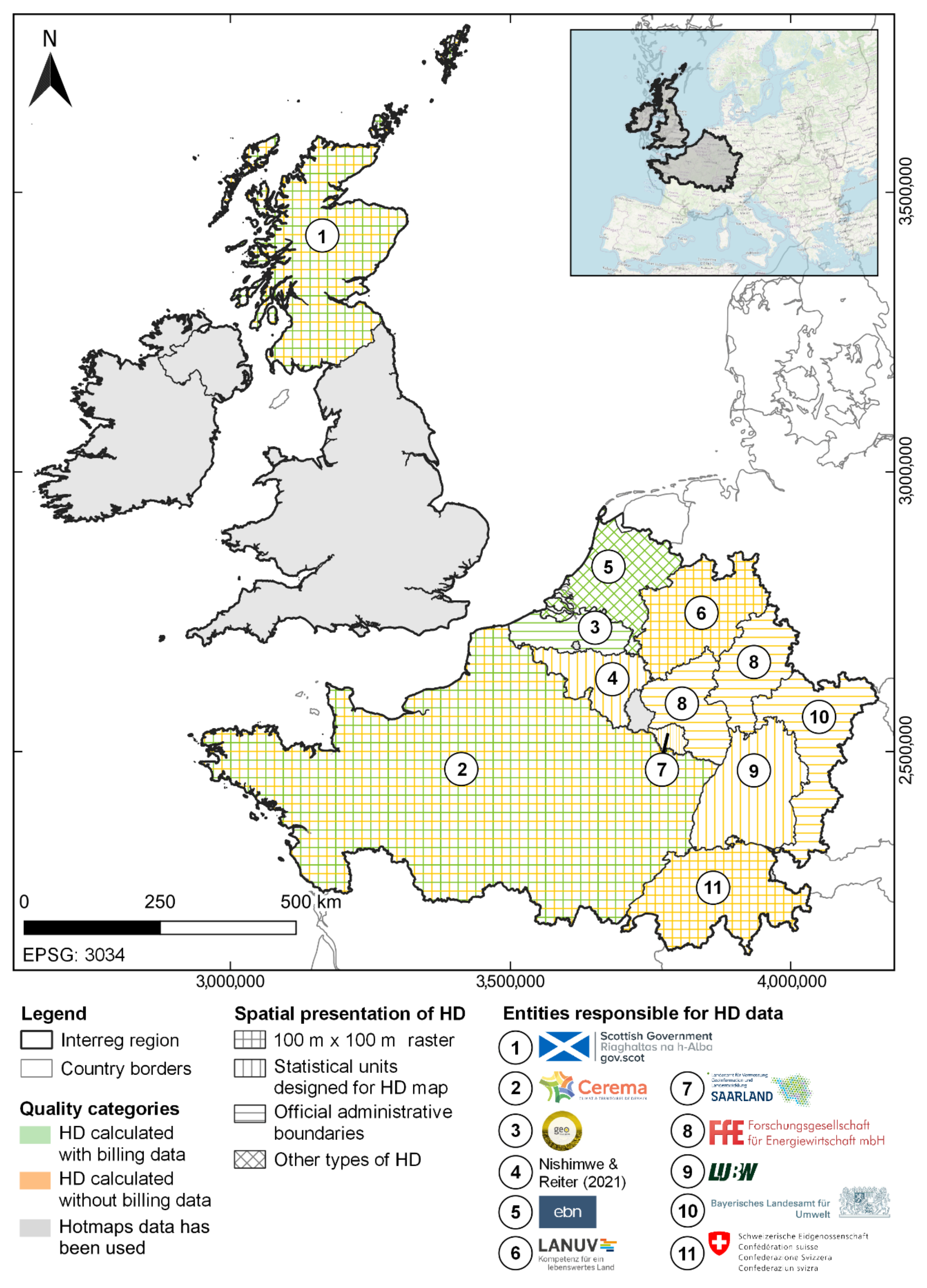
To address a scenario in which local to regional heat demand analyses with appropriate and user-friendly tools will become mandatory, this study has been conducted within the framework of the Interreg North-West-Europe area (Interreg NWE) project “Roll-out of Deep Geothermal Energy in North-West-Europe” (DGE-ROLLOUT) [6,7,8,9]. As part of the project, the goal of this study was to produce harmonized heat demand maps for the project area on one hand, and thereby develop a sufficient method that can be used for tool-development for heat demand analysis on variable input datasets and scales on the other hand. According to the Energy Efficiency Directive, the member states of the EU must map their HD on a high spatial resolution [10]. National HD data of several member and non-member states were available for this study (Belgium [11], Switzerland [12], Germany [13,14,15,16,17], France [18], The Netherlands [19,20], and Scotland [21]).

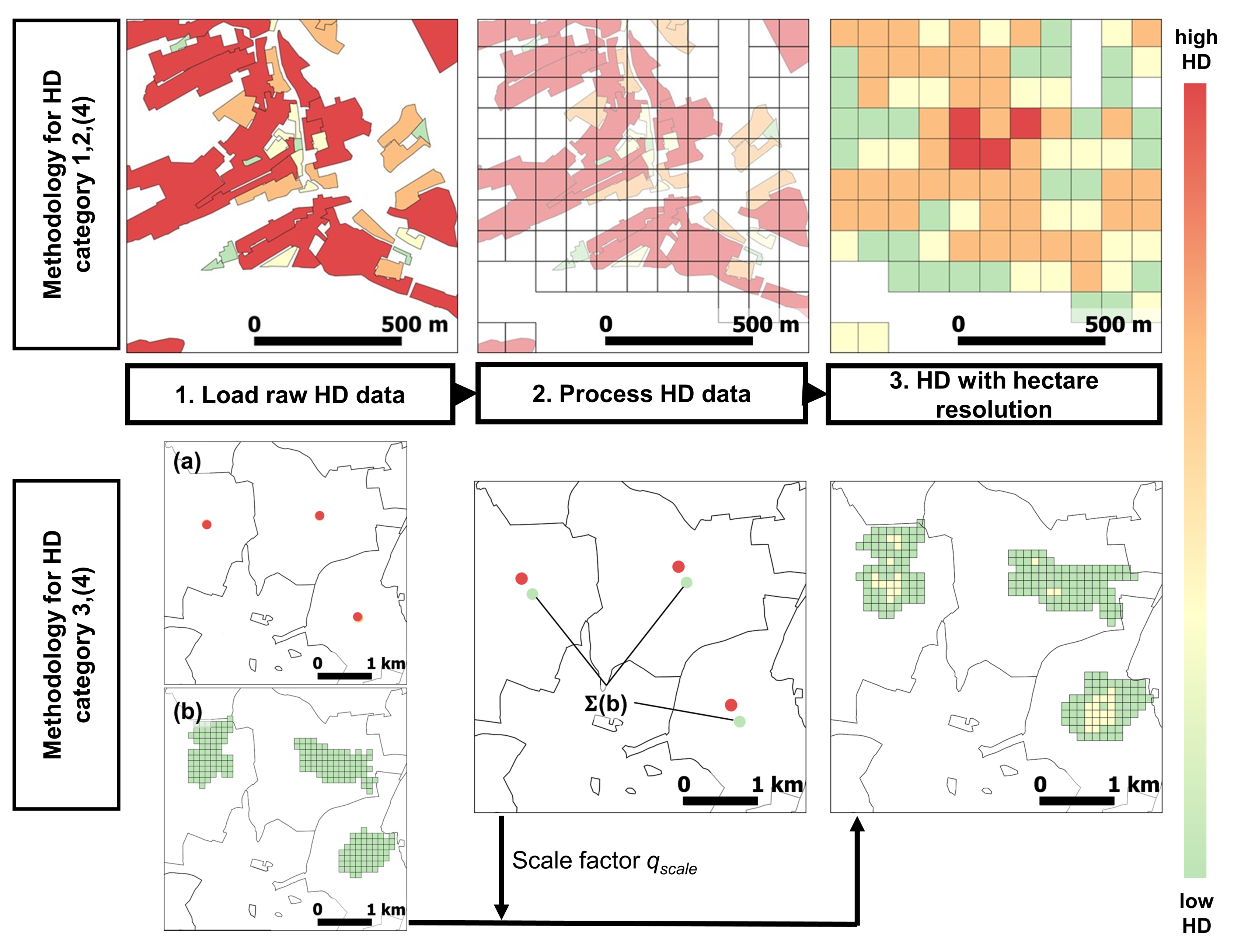
The HD describes the energy in megawatt hours (MWh) needed for space and water heating over a certain area (e.g., 100 m × 100 m = 1 ha) and time period (e.g., one year after the Julian calendar with 365/366 days). Usually, the heating differs between the residential/domestic and commercial sectors. Residential buildings are exclusively used for private usage, e.g., single- or multi-family buildings. Commercial buildings refer to any property used for business activity, e.g., office, retail, and lodging. The commercial sector on the DGE-ROLLOUT HD map also includes some institutional buildings, e.g., medical, educational, religious, and governmental buildings. While minor contributions of process heat may be included in the heat demand input data for these buildings, large industrial processes or processes that require large amounts of heat are not included. Industrial, military, and infrastructural buildings are not included in the HD maps as their data are not publicly available and require individual approaches to characterize the heat sources and sinks, e.g., via a pinch analysis.

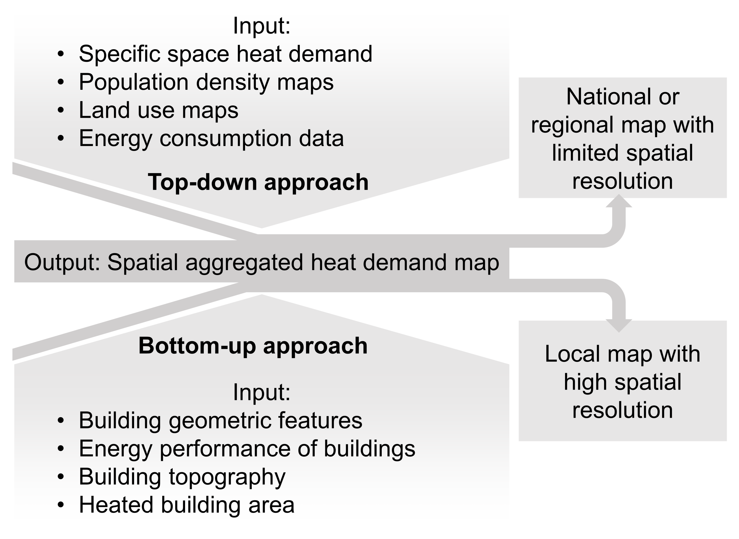
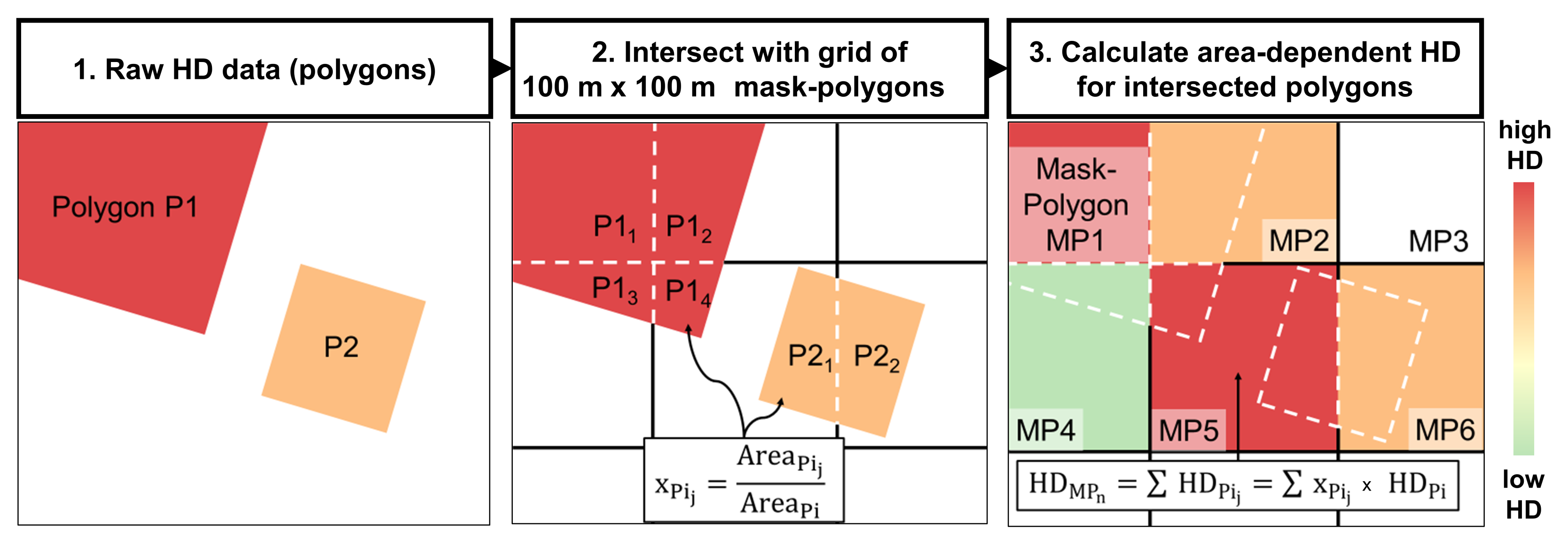
For the development of an HD map, a top-down or a bottom-up approach can be used, which differ fundamentally in their methodology (Figure 1). The first calculates HD on a large scale, usually on a national level or on lower Nomenclature of Territorial Units for Statistics (NUTS), while using publicly available, low-resolution data. The latter uses high-resolution data on a regional level, usually a city or a Local Administrative Unit (LAU). However, this more detailed approach significantly increases the computational and processing requirements. Because this might represent a hurdle for many municipalities in local to regional heat demand analysis as a fundamental element of municipal heat planning, methodological simplifications as preparation for the implementation of end-user tools are inevitable.

The two projects with the largest and most comprehensive dataset for spatial mapping of HD on a European level are Hotmaps [23] and the Pan European Thermal Atlas of Heat Roadmap Europe (HRE) [24]. Both projects use well-designed top-down approaches, based on a strong level of scientific expertise [25,26,27,28,29]. The Hotmaps project uses a statistical approach, whereas HRE uses an econometric approach. Both projects present their resulting heat demands on hectare resolution (100 m × 100 m). Besides these two projects, the development of HD maps has become an emerging subject of research in recent years. A profound literature review of HD maps until 2019 has been compiled by [30]. A detailed analysis is usually done at the city or district level, aiming at evaluating the (pre-) feasibility of district heating systems or regional development plans [31,32,33,34]. The traditional approach to developing HD maps is to use a geographic information system such as QGIS or ArcGIS [22,35,36]. Recently, more approaches using scripting languages, like R or Python, have appeared [37,38,39]. Since the datasets and methodologies are usually not publicly accessible, these local studies were not included in this study. An exception is a recent study for the Walloon region in Belgium, where no other HD data are available [40]. Many of the aforementioned studies do not provide the tools (i.e., scripts) to replicate the results. Further, they usually focus on smaller regions whereas the developed methodology in this study is not restricted to any administrative level or level of resolution.

Within the framework of this study, the open-source Python package PyHeatDemand was developed [41]. Rather than aiming to replace any existing heat demand mapping methods, it focuses on providing a methodology for administrative entities to harmonize heat demand data, thereby improving district heating plans. Three HD maps of the Interreg NWE area are presented in this study, applying the developed procedures using publicly available consumption data to identify hotspots of the residential HD and the commercial HD, and both combined on a hectare scale for the observation period of one year (Julian calendar). The developed approach is easy to apply to different categories of data and allows for the reproducibility of the outcomes, a constant update of the maps once new data becomes available, and an extension of the study area for previously unmapped territory. The resulting HD maps are validated against the HD maps from Hotmaps and HRE (only a top-down approach). A combination of a bottom-up and top-down approach is implemented to deliver a higher resolved result than previous mapping projects. Major sweet spots for investment projects, for example, heat production from deep geothermal power plants using doublet systems or the extension of existing or development of new district heating systems, are assumed in areas with a high degree of urbanization, as these areas have usually existing district heating networks and a high customer density.

2. Materials and Methods

2.1. General Heat Demand Map Workflow

The creation of the heat demand maps follows a general workflow (Figure 2) followed by a data-category-specific workflow for the five defined heat demand input data categories (Table 1). Depending on the scale of the heat demand map (local, regional, national, or even transnational), a global polygon mask is created from the provided administrative boundaries for the entire administrative unit (Interreg NWE region) with a cell size of 10 km by 10 km, for instance, and the target coordinate reference system (CRS, ETRS89-extended/LCC Europe—EPSG:3034). This mask is used to divide the study area into smaller chunks for a more reliable processing as only data within each mask will be processed separately. If necessary, the global mask will be cropped to the extent of the available heat demand input data and populated with polygons having already the final cell size such as 100 m × 100 m. Refining a previously coarser polygon mask is achievable by employing a self-implemented QuadTree algorithm [42], continuing the process until reaching the final resolution, such as 100 m × 100 m. In that case, only the areas with a high data density will display cell sizes of the final resolution while areas of low data densities will be combined. This also allows for identifying areas with only a few data points but large heat demands and vice versa. For each cell, the cumulated heat demand will be calculated. This was first done without utilizing spatial indexing. At a later stage, spatial indices [RTree] [43] were implemented with a significant decrease in computing times. The final regular polygon grid will be rasterized and merged with adjacent global cells to form a mosaic, the final local to transnational heat demand map. If several input datasets are available for a region, i.e., different sources of energy, they can either be included in the calculation of the heat demand or the resulting rasters can be added to a final heat demand map.

The QGIS long-term release [v. 3.28.11] [44] is used to perform simple spatial operations to verify the processability and quality of the generated data. Python [v. 3.10.] [45] including different open-source libraries such as GeoPandas [v. ≥ 0.14.0] and Shapely [v. > 2.0.2] [46,47] are used for processing the data, in particular for advanced geospatial operations and analysis. The Rasterio package [v. ≥ 1.3.9] [48] is further used to create the raster data. The developed workflow can be executed in Jupyter Python Notebooks [49] allowing for reproducible outcomes or recomputation of the results once new input data is available. All methods required to create the heat demand maps are also available in the open-source Python package PyHeatDemand [41] referenced in the Data Availability Statement, which was created within the framework of the DGE-ROLLOUT project. The pure Python implementation guarantees the reproducibility of the results and eliminates manual data manipulation in geoinformation systems, which are now only used for verification, quality control, and map creation.

Table 1. Different spatial categories of the provided heat demand data for the DGE-ROLLOUT project. The exact citation can be found in the references.

Data Category	Description	Regions (ISO 3166 [50]) and Prev. Studies
1	HD data provided as (e.g., 100 m × 100 m) raster or polygon grid with the same or in a different coordinate reference system	CH [12], FR [18], DE-NW [16], UK-SCT [21], Hotmaps [23], HRE [24]
2	HD data provided as building footprints or street segments	BE-VLG [11], DE-BW [13], DE-SL [17] including industrial parts
3	HD data provided as a point or polygon layer, which contains the sum of the HD for regions of official administrative units	DE-BY [15], DE-HE, and DE-RP [14]
4	HD data provided in other data formats such as HD data associated with addresses	NL [19,20], BE-WAL [40]
5	No HD data available for the region	Luxembourg, United Kingdom (excluding Scotland)

Table 1. Different spatial categories of the provided heat demand data for the DGE-ROLLOUT project. The exact citation can be found in the references.

Data Category	Description	Regions (ISO 3166 [50]) and Prev. Studies
1	HD data provided as (e.g., 100 m × 100 m) raster or polygon grid with the same or in a different coordinate reference system	CH [12], FR [18], DE-NW [16], UK-SCT [21], Hotmaps [23], HRE [24]
2	HD data provided as building footprints or street segments	BE-VLG [11], DE-BW [13], DE-SL [17] including industrial parts
3	HD data provided as a point or polygon layer, which contains the sum of the HD for regions of official administrative units	DE-BY [15], DE-HE, and DE-RP [14]
4	HD data provided in other data formats such as HD data associated with addresses	NL [19,20], BE-WAL [40]
5	No HD data available for the region	Luxembourg, United Kingdom (excluding Scotland)

2.2. Data Categories 1 and 2

The processing of data categories 1 and 2 follows similar workflows and corresponds to a bottom-up approach. The heat demand input data of category 1 are already displayed as a raster or a polygon grid, usually with a spatial resolution of 100 m × 100 m. The raster will be vectorized to continue working with a polygon grid containing the heat demand data. The heat demand input data of category 2 are buildings of similar age classes and energy requirements, grouped as one statistical unit containing the heat demand data (Figure 3(1) and Figure 4 top). Further, the heat demand data can also be represented as street segments (LineStrings). Both data categories (1 & 2) are intersected with a local mask layer consisting of 100 m × 100 m polygons (Figure 3(2)) or a different target resolution. This results in individual polygon fragments $P_i$ inside each mask-polygon j. The HD of the intersected statistical units is summed up for each mask polygon $H{D}_{M{P}_n}$ and calculated according to their share of area $x_j$ (Figure 3(3), Equation (1)).

For regions that have not provided any input heat demand data, the Hotmaps HD data has been used in this study instead. Since Hotmaps data is given with a high spatial resolution of 100 m × 100 m raster cells in a different CRS, the methodology is identical as for HD of category 1. If no heat demand input data is available at all, top-down or bottom-up workflows can be utilized to estimate the heat demand (see section below).

$$H{D}_{M{P}_n}=\sum H{D}_{P{i}_j}=\sum x_{P{i}_j}·H{D}_{Pi}$$

(1)

2.2.1. Data Category 3

HD data of category 3 is provided as a point or polygon layer, where each point or polygon represents the sum of the HD for regions at the Local Administration Units level (LAU) for this study or any other administrative unit. The processing of this data corresponds to a top-down approach. The centroids of the polygons are then used for further processing. The spatial distribution of HD from Hotmaps is used to increase the resolution to 100 m × 100 m. These Hotmaps data are summed up for each LAU and then compared with the provided heat demand input data. Equation (2) defines a scale factor $q_{scale}$ for each LAU as the heat demand input data $H{D}_{provided}$ is divided by the summed-up Hotmaps HD data $H{D}_{\Sigma Hotmaps}$. Each Hotmaps HD grid cell is then multiplied with this scale factor. This process increases the spatial resolution of the provided heat demand input data using the solid scientific approach from Hotmaps (Figure 4). Alternatively, population density grids can be utilized to increase the spatial resolution of the data.

$$q_{scal{e}_{LAU}}=\frac{H{D}_{provided}}{H{D}_{\sum Hotmaps}}$$

(2)

2.2.2. Data Category 4

Category 4 comprises all the unique processing methods for HD data, which could not be categorized within the previous formats. The calculation of HD for instance for the Netherlands as presented later is based on the absolute gas demand per postal code area. Gas is used for 84% of heat generation in the residential sector and as a total energy carrier [19,20]. Equation (3) has been defined to transform the gas demand into heat demand:

$$H{D}_{NL}=\eta \times C{V}_{net}\times (SH+HW)\times G{D}_{NL}$$

(3)

$H{D}_{NL}$ refers to the annual HD in the Netherlands in MWh/ha. $G{D}_{NL}$ is the gas demand in m${}^3$/a. $C{V}_{net}$ is the net calorific value of natural gas, which is set to 31.65 MJ/m${}^3$ or, to use the correct unit directly, 8.79 kWh/m${}^3$ for this region [51]. An efficiency factor $\eta$ is used to account for the inefficiency of gas-fired systems. However, the efficiency factor was set to $\eta =100\%$ for this study. The fraction of gas used for space heating $SH$ and hot water heating $HW$ is set to 72.7% and 23.3% [52,53], respectively. The remaining 4% are attributed to the usage of gas for cooking purposes [52].

Using gas usage or the usage of any source of heat can be converted into a heat demand and corresponds to a very precise bottom-up approach using billing data. This becomes increasingly important with more and more decentralized and independent heat sources. The resulting heat demands for each energy source can later be aggregated to result in the final heat demand of a respective local cell.

For the Walloon region as another example, the HD is provided for each NUTS-3 region as image data [40]. This image data is georeferenced and the color code of each NUTS-3 is extracted as point data. The HD of each point corresponds to the predefined value ranges, here, the lower limit, defined by Ref. [40]. The point layer has been manually adjusted where the color code extraction was not successful. This point layer is used as the input for processing HD in category 3.

2.3. Development of the Heat Demand Maps

The development of the workflow to create three standardized maps for the DGE-ROLLOUT project showing the annual heat demand on a hectare resolution (in MWh/ha/a as 100 m × 100 m) is based on existing regional heat demand input data displaying a wide range of possible data formats. The regionally collected consumption data is publicly available through project partners, authorities, and research communities. In comparison to previous projects, real measurement data (billing data) is implemented to represent the spatial conditions as accurately as possible. The residential and commercial heat demands include heat demands for space heating and hot water. No industrial processes or process heat are included in the dataset if not stated otherwise (e.g., Saarland).

The provided HD data can be divided into two categories of quality and five categories of spatial presentation, based on the region (according to Ref. [50]) or the previous studies (Hotmaps, Heat Roadmap Europe), respectively (Table 1). The two categories of quality depend on whether the provided heat demand input data is calculated or originates from billing data (Figure 5). The latter can be interpreted as a bottom-up approach.

Since the heat demand input data is usually provided in a regional coordinate reference system (CRS), it has been transformed into the reference system used by the DGE-ROLLOUT project (ETRS89-extended/LCC Europe—EPSG:3034) to avoid distortions of the spatial data.

2.4. Statistical Evaluations Using Rasterstats Library

The compiled heat demand maps were analyzed on a national scale using the zonal statistics of the Rasterstats Python library [54] in combination with simple algebraic calculations using the Pandas Python library [55]. Hereby, the zonal statistics only account for raster cells that actually hold a value. Cells, where no heat demand has been calculated, are not considered in these calculations.

Zonal statistics cannot only be applied on a national level but also on a regional level (e.g., states, communes) or a local level (cities, districts) to evaluate and summarize the respective heat demand for heat demand planning.

2.5. Development of Heat Demand Difference Maps

To further evaluate the quality of the merged DGE-ROLLOUT HD maps, Hotmaps and HRE have been used as references. The HD data from these projects are provided as 100 m × 100 m raster cells for the entire region of this study but were using a top-down approach rather than using the combined bottom-up and top-down approach also integrating billing data like for this study. The transformation of these HD data is identical to HD data from category 1. Each 100 m × 100 m raster cell from each DGE-ROLLOUT HD map has been subtracted from their Hotmaps and HRE counterparts to develop the difference maps (Figure 6). Equation (4) describes the HD difference $H{D}_{diff}$ for each raster cell.

$$H{D}_{diff}=H{D}_{DGE-ROLLOUT}-H{D}_{\frac{Hotmaps}{HRE}}$$

(4)

The statistical dispersion of the average HD differences between the DGE-ROLLOUT and Hotmaps/HRE is presented in the form of violin plots, presenting a probability density of the HD differences. Six violin plots, two each for the residential, commercial, and total HD difference maps (HDDM) display the statistical dispersion. The plots present the mean values and the corresponding standard error of means as a distribution. Furthermore, the median of the mean values and the 25th and 75th quantiles are outlined.

3. Results

3.1. Heat Demand Maps

Using the developed workflow including the implementation of spatial indices, three maps developed in this study present the HD in units of energy over a certain area (100 m × 100 m raster cells) and time period for the residential and commercial sectors and the summed-up HD of both sectors (Figure 7). Since the time period is always one year (Julian calendar), it is usually not displayed for the annotation of the units. HD values below 15 MWh/ha are not displayed in the maps, due to calculation inaccuracies and low significance for investment projects. While the areas with heat demands below 15 MWh/ha account for 44.3% (residential), 51.2% (commercial), and 38.9% (combined) of the area that is covered by heat demand, they only account for 2.18%, 2.80%, and 1.48% of the respective heat demands. These areas are located in sparsely populated areas and at the edge of more densely populated areas. Data tables summarizing the heat demand data are available in the Appendix A.

3.1.1. Areal Statistics

Areal statistics are presented prior to the results of the heat demand mapping. As the resulting maps extend over larger parts of Europe, the ellipsoidal area measurements accounting for the curvature of the earth when working on a larger scale are favored over the planimetric measurements usually used for local area calculations. The ellipsoidal areas were extracted from QGIS and implemented in the statistical analysis instead of using the planimetric values calculated by the designated GeoPandas and Shapely libraries [46,47] as they use the planimetric area measurement approach. Overall, the planimetric area data only measures around 93% of the ellipsoidal area. Hence, there would have been a significant error when using the planimetric measurements. The total area of the Interreg NWE region amounts to 842,824 km${}^2$. The northern part of France contributes 33.1% (279,030 km${}^2$) followed by Great Britain with 19.6% (165,486 km${}^2$) and the western part of Germany with 17.4% (146,607 km${}^2$). The remaining countries contribute with less than 10% each to the total Interreg NWE region with as little as 0.3% (2596 km${}^2$) for Luxembourg (

Table A1. Statistical values for the total heat demand of the Interreg NWE region.

Region	Area (Planimetric) [km${}^2$]	Area (Ellipsoidal) [km${}^2$]	Share of Total Area [%]	Combined/Total HD [TWh]	Share of Total HD [%]	Average of Total HD [MWh/ha]	Average of Heated Area of Total HD [MWh/ha]	Area of Heat Demand [km${}^2$]	Share of Heated Heat Demand Area [%]	Population
Interreg NWE	788,016	842,824	100	1727.2	100	20.5	127.4	135,542	16.1	191,933,967
Germany	136,800	146,607	17.4	606.8	35.1	41.4	186.1	32,613.9	22.2	46,252,822
Great Britain	154,556	165,486	19.6	422.6	24.5	25.5	159.3	26,529.6	16.0	60,316,107
France	260,768	279,030	33.1	362.4	21	13	71.2	50,934.6	18.3	39,344,973
Belgium	28,595	30,665	3.6	106.4	6.2	34.7	138.5	7680.8	25.0	11,364,385
Switzerland	38,663	41,263	4.9	74.2	4.3	18	197.8	3749.5	9.1	8,615,805
Netherlands	26,826	28,755	3.4	74	4.3	25.7	139.9	5289.4	18.4	1,5414,496
Scotland	74,237	78,684	9.3	40.7	2.4	5.2	110.7	3681.6	4.7	5,348,404
Ireland	65,150	69,738	8.3	32.5	1.9	4.7	71.2	4572.7	6.6	4,675,657
Luxembourg	2421	2596	0.3	7.5	0.4	29	153.8	490.3	18.9	601,318

,

Table A2. Statistical values for the residential heat demand of the Interreg NWE region.

Region	Area (Planimetric) [km${}^2$]	Area (Ellipsoidal) [km${}^2$]	Share of Total Area [%]	Residential HD [TWh]	Share of Residential HD [%]	Average of Residential HD [MWh/ha]	Average of Heated Area of Residential HD [MWh/ha]	Area of Heat Demand [km${}^2$]	Share of Heated Heat Demand Area [%]
Interreg NWE	788,016	842,824	100	1129.3	100	13.4	91.0	124,161	14.7
Germany	136,800	146,607	17.4	340.3	30.1	23.2	123	27,673.1	18.9
Great Britain	154,556	165,486	19.6	320.6	28.4	19.4	120.8	26,529.4	16
France	260,768	279,030	33.1	266.7	23.6	9.6	54	49,371.1	17.7
Belgium	28,595	30,665	3.6	75.3	6.7	24.6	98.6	7640.9	24.9
Netherlands	26,826	28,755	3.4	52.2	4.6	18.2	122.8	4250.3	14.8
Switzerland	38,663	41,263	4.9	47.3	4.2	11.5	130.1	3636.8	8.8
Ireland	65,150	69,738	8.3	22.1	2	3.2	48.3	4569.1	6.6
Luxembourg	2421	2596	0.3	4.8	0.4	18.4	97.5	490.2	18.9
Scotland	74,237	78,684	9.4	No data	No data	No data	No data	No data	No data

and

Table A3. Statistical values for the commercial heat demand of the Interreg NWE region.

Region	Area (Planimetric) [km${}^2$]	Area (Ellipsoidal) [km${}^2$]	Share of Total Area [%]	Commer- cial HD [TWh]	Share of Commercial HD [%]	Average of Commercial HD [MWh/ha]	Average of Heated Area of Commercial HD [MWh/ha]	Area of Heat Demand [km${}^2$]	Share of Heated Heat Demand Area [%]
Interreg NWE	788,016	842,824	100	557.1	100	6.6	70.2	79,312	9.4
Germany	136,800	146,607	17.4	266.4	47.8	18.2	94.3	28,263.4	19.3
Great Britain	154,556	165,486	19.6	102	18.3	6.2	38.5	26,529.4	16
France	260,768	279,030	33.1	95.7	17.2	3.4	92.8	10,316.7	3.7
Belgium	28,595	30,665	3.6	31.1	5.6	10.1	72.1	4314.9	14.1
Switzerland	38,663	41,263	4.9	26.9	4.8	6.5	96.3	2788.5	6.8
Netherlands	26,826	28,755	3.4	21.8	3.9	7.6	106.9	2039.4	7.1
Ireland	65,150	69,738	8.3	10.4	1.9	1.5	22.7	4569.1	6.6
Luxembourg	2421	2596	0.3	2.8	0.5	10.6	56.3	490.2	18.9
Scotland	74,237	78,684	9.4	No data	No data	No data	11.9	0.1	0

). Neglectable area differences occur between the regional areas and the national areas. The latter ones have a total planimetric area that is 4 km${}^2$ larger and an ellipsoidal area that is 1 km${}^2$ larger than the regional areas. This difference arose during the creation of the national layer.

3.1.2. National Results—Level 0 of the Nomenclature of Territorial Units for Statistics

The total HD (residential and commercial combined) of the Interreg NWE region is approximately 1727.2 TWh (Table A1). The residential HD accounts for 65.38% (1129.3 TWh, Table A2) while the commercial HD accounts for 32.26% (557.1 TWh, Table A3). The remaining 2.35% are attributed to the HD of Scotland (40.7 TWh) which was only provided as total HD and was not split in residential or commercial HD, respectively. The country with the highest total heat demand is Germany (only the NWE part) with 606.9 TWh (35.1% of the total HD) split into 340.3 TWh (30.1% of residential HD) and 266.5 TWh (41.4% of commercial heat demand, Figure 8). Here, it is worthwhile mentioning that the state of Saarland also contributes industrial heat demand to the total HD.

The two other major consumers are Great Britain with 24.5% of the total heat demand, 28.4% of the residential heat demand, and 18.3% of commercial heat demand, and France (only NWE part) with 21.0%, 23.6%, and 17.2%, respectively (Figure 8). These three countries account for ∼80% of all three calculated heat demands as they also account for 76.0% of the total Interreg population [56]. The remaining countries have shares ranging from 0.4% (7.5 MWh/ha total) to 6.7% (75.3 MWh/ha residential) for all three HD categories (Figure 8). The share of the residential HD to the total HD ranges between 63.4% (Luxembourg) and 75.9% Great Britain (2/3 to 3/4). In return, the commercial heat demand only accounts for 24.1% (Great Britain) to 36.6% of the total heat demand (1/4 to 1/3). In Germany as an exception, the share of the commercial sector accounts for 43.9% while the residential sector only accounts for 56.1% of the total heat demand.

The total average heat demand for the entire Interreg NWE region (842,824 km²) equals 20.5 MWh/ha. This corresponds to 13.4 MWh/ha and 6.6 MWh/ha for the residential and commercial heat demand. The missing 0.5 MWh/ha can be attributed once again to Scotland where only the total HD was provided. Splitting this into the values for the different countries indicates that Germany (41.4 MWh/ha, 23.2 MWh/ha, 18.2 MWh/ha) and Belgium (34.7 MWh/ha, 24.6 MWh/ha, 10.1 MWh/ha) have the highest average heat demands. They are followed by Luxembourg, the Netherlands, Great Britain, and Switzerland. Compared to Germany, the average heat demands of France are much lower at 13.0 MWh/ha, 9.6 MWh/ha, and 3.4 MWh/ha. The lowest average total heat demands with approximately 5 MWh/ha are present in Ireland and Scotland.

Using zonal statistics, it is possible to calculate statistics only for the areas of each country that actually have heat demand values present. These reveal that only 16.1% (135,542 km${}^2$) of the Interreg NWE region have heat demand values present (residential and commercial combined). In return, 83.9% (707,282 km${}^2$) remains unused land. The actual heated area results in an average total heat demand of 127.4 MWh/ha compared to 20.5 MWh/ha when taking the entire Interreg NWE region into account. This also results in higher average total heat demand values for the respective countries with values ranging from 71.2 MWh/ha for France to 197.8 MWh/ha for Switzerland. The share of the heated heat demand area in the single countries ranges from 4.7% for Scotland, indicating a low heat demand density, and up to 25.0% for Belgium, indicating that heat demand is present in 1/4 of the country. Dividing this into residential and commercial heat demand results in areas of 14.7% (124,161 km${}^2$) and 9.4% (79,312.0 km${}^2$), respectively. The shares range excluding Scotland from 6.6% for Luxembourg to 24.9% for Belgium and from 3.7% for France and 19.3% for Germany, respectively.

3.1.3. Regional Results—Level 1 of the Nomenclature of Territorial Units for Statistics

The regional results are evaluated on a comparable NUTS 1 Level (Table A2, Table A3,

Table A4. Summary of the heat demand data for the total HD of the Interreg NWE region.

Region	Region Name	Area (Planimetric) [km${}^2$]	Area (Ellipsoidal) [km${}^2$]	Share of Total Area [%]	Combined/Total HD [TWh]	Share of Total HD [%]	Average of Total HD [MWh/ha]	Average of Heated Area of Total HD [MWh/ha]	Area of Heat Demand [km${}^2$]	Share of Heated Heat Demand Area [%]
Interreg NWE	Interreg NWE	788,012	842,823	100	1727.2	100	20.5	127.4	135,542	16.1
DEA	Nordrhein-Westfalen	31,807	34,106	4	218.6	12.7	64.1	191.2	11,434.4	33.5
DE1	Baden-Württemberg	33,587	35,961	4.3	128.7	7.5	35.8	168.6	7636	21.2
FR1	Ile-de-France	11,268	12,068	1.4	92.1	5.3	76.3	299.2	3077.4	25.5
DE7	Hessen	19,678	21,102	2.5	84.9	4.9	40.2	218	3896.1	18.5
DE2	Bayern	30,810	33,012	3.9	77.9	4.5	23.6	145.6	5348.8	16.2
CH0	Switzerland	38,663	41,263	4.9	74.2	4.3	18	197.8	3749.5	9.1
BE2	Vlaams Gewest	12,678	13,597	1.6	72.5	4.2	53.3	207.7	3490.3	25.7
DEB	Rheinland-Pfalz	18,518	19,853	2.4	62.5	3.6	31.5	167.4	3735.8	18.8
UKJ	South East (England)	17,816	19,105	2.3	62.3	3.6	32.6	141.6	4395.6	23
FRF	Grand Est	53,904	57,725	6.8	55.2	3.2	9.6	89.7	6152.2	10.7
UKI	London	1470	1577	0.2	52.7	3.1	334.1	429.3	1227.3	77.8
UKD	North West (England)	13,227	14,139	1.7	52.3	3	37	177.6	2945.4	20.8
FR-HDF	Hauts-de-France	29,779	31,927	3.8	50.9	2.9	15.9	86.6	5881.5	18.4
FRD	Normandie	28,055	30,060	3.6	44.1	2.6	14.7	58.3	7560.4	25.2
UKH	East of England	17,869	19,151	2.3	42.6	2.5	22.2	137.8	3089	16.1
UKG	West Midlands (England)	12,144	13,013	1.5	41.7	2.4	32.1	156.5	2665.7	20.5
FR-PDL	Pays de la Loire	30,248	32,329	3.8	41.5	2.4	12.8	53.4	7761.3	24
UKM	Scotland	74,237	78,684	9.4	40.7	2.4	5.2	110.7	3681.6	4.7
UKE	Yorkshire & the Humber	14,431	15,429	1.8	40.2	2.3	26	184.1	2182.4	14.1
UKK	South West (England)	22,278	23,891	2.8	39.7	2.3	16.6	126.2	3149.9	13.2
NL3	West-Nederland	9351	10,023	1.2	37.2	2.2	37.1	184.8	2011.2	20.1
DEC	Saarland	2400	2573	0.3	34.1	2	132.4	605.4	562.8	21.9
UKF	East Midlands (England)	14,604	15,641	1.9	34	2	21.7	151.3	2246	14.4
IE0	Ireland	65,150	69,738	8.3	32.5	1.9	4.7	71.2	4572.7	6.6
FRC	Bourgogne-Franche-Comte	44,977	48,048	5.7	28.5	1.6	5.9	46.5	6122.7	12.7
FR-BRE	Bretagne	25,558	27,352	3.2	27	1.6	9.9	31.8	8474.5	31
UKL	Wales	19,415	20,806	2.5	24.3	1.4	11.7	135.2	1797.4	8.6
FRB	Centre-Val de Loire	36,977	39,520	4.7	23.3	1.3	5.9	39.4	5904.6	14.9
UKC	North East (England)	8069	8606	1	20.4	1.2	23.8	183.2	1116	13
NL4	Zuid-Nederland	6801	7293	0.9	19.6	1.1	26.9	130.8	1498.4	20.5
BE3	Region wallonne	15,765	16,905	2	19.2	1.1	11.4	47.3	4056.8	24
NL2	Oost-Nederland	10,232	10,966	1.3	17.2	1	15.7	97	1775.1	16.2
BE1	Region de Bruxelles-Capitale/Brussels Hoofdstedelijk Gewest	151	162	0	14.7	0.9	908.6	1101.5	133.6	82.5
UKN	Northern Ireland	13,232	14,128	1.7	12.4	0.7	8.8	72.2	1714.7	12.1
LU0	Luxembourg	2421	2596	0.3	7.5	0.4	29	153.8	490.3	18.9
NL1	Noord-Nederland	442	474	0.1	0	0	0.8	85	4.7	1

,

Table A5. Summary of the heat demand data for the residential HD of the Interreg NWE region.

Region	Region Name	Area (Planimetric) [km${}^2$]	Area (Ellipsoidal) [km${}^2$]	Share of Total Area [%]	Residential HD [TWh]	Share of Residential HD [%]	Average of Residential HD [MWh/ha]	Average of Heated Area of Residential HD [MWh/ha]	Area of Heat Demand [km${}^2$]	Share of Heated Heat Demand Area [%]
Interreg NWE	Interreg NWE	788,012	842,823	100	1110.1	100	13.2	90.7	122,364	14.5
DEA	Nordrhein-Westfalen	31,807	34,106	4	136.1	12.3	39.9	138.4	9837.6	28.8
DE2	Bayern	30,810	33,012	3.9	64.5	5.8	19.5	120.5	5348.3	16.2
DE1	Baden-Württemberg	33,587	35,961	4.3	55.1	5	15.3	125.4	4393.6	12.2
FR1	Ile-de-France	11,268	12,068	1.4	54.9	4.9	45.5	190.1	2887.5	23.9
BE2	Vlaams Gewest	12,678	13,597	1.6	53	4.8	39	153.7	3450.6	25.4
CH0	Switzerland	38,663	41,263	4.9	47.3	4.3	11.5	130.1	3636.8	8.8
UKJ	South East (England)	17,816	19,105	2.3	45.3	4.1	23.7	103.1	4395.6	23
DE7	Hessen	19,678	21,102	2.5	42.5	3.8	20.1	109	3895.9	18.5
FRF	Grand Est	53,904	57,725	6.8	42	3.8	7.3	71.2	5890.8	10.2
UKI	London	1470	1577	0.2	40.9	3.7	259.2	333	1227.3	77.8
UKD	North West (England)	13,227	14,139	1.7	40.8	3.7	28.8	138.5	2945.4	20.8
FR-HDF	Hauts-de-France	29,779	31,927	3.8	38.3	3.4	12	67.5	5670.3	17.8
FRD	Normandie	28,055	30,060	3.6	37.7	3.4	12.5	50.9	7394.7	24.6
FR-PDL	Pays de la Loire	30,248	32,329	3.8	33.5	3	10.4	44.5	7530.5	23.3
UKH	East of England	17,869	19,151	2.3	31.6	2.9	16.5	102.5	3089	16.1
UKG	West Midlands (England)	12,144	13,013	1.5	31.5	2.8	24.2	118	2665.7	20.5
DEB	Rheinland-Pfalz	18,518	19,853	2.4	31.3	2.8	15.8	83.7	3735.7	18.8
UKE	Yorkshire & the Humber	14,431	15,429	1.8	30.5	2.7	19.8	139.8	2182.4	14.1
UKK	South West (England)	22,278	23,891	2.8	29.4	2.6	12.3	93.3	3149.9	13.2
UKF	East Midlands (England)	14,604	15,641	1.9	26	2.3	16.6	115.9	2246	14.4
NL3	West-Nederland	9351	10,023	1.2	25.6	2.3	25.6	158.6	1616.4	16.1
IE0	Ireland	65,150	69,738	8.3	22.1	2	3.2	48.3	4569.1	6.6
FR-BRE	Bretagne	25,558	27,352	3.2	21.3	1.9	7.8	25.6	8301.6	30.4
FRC	Bourgogne-Franche-Comte	44,977	48,048	5.7	20.9	1.9	4.4	35.2	5947	12.4
FRB	Centre-Val de Loire	36,977	39,520	4.7	18.2	1.6	4.6	31.7	5748.8	14.5
UKC	North East (England)	8069	8606	1	16	1.4	18.6	143.3	1116	13
BE3	Region wallonne	15,765	16,905	2	14.4	1.3	8.5	35.5	4056.7	24
NL4	Zuid-Nederland	6801	7293	0.9	13.9	1.3	19.1	114.4	1218.5	16.7
NL2	Oost-Nederland	10,232	10,966	1.3	12.6	1.1	11.5	89.4	1412.3	12.9
DEC	Saarland	2400	2573	0.3	10.9	1	42.5	237	462	18
UKN	Northern Ireland	13,232	14,128	1.7	9.4	0.8	6.6	54.6	1714.7	12.1
BE1	Region de Bruxelles-Capitale/Brussels Hoofdstedelijk Gewest	151	162	0	7.9	0.7	485.2	588.2	133.6	82.5
LU0	Luxembourg	2421	2596	0.3	4.8	0.4	18.4	97.5	490.2	18.9
NL1	Noord-Nederland	442	474	0.1	0	0	0.5	70.1	3.1	0.7
UKM	Scotland	74,237	78,684	9.4	No data	No data	No data	35.8	0.1	0
UKL	Wales	19,415	20,806	2.5	0	0	0	0	0	0

and

Table A6. Summary of the heat demand data for the commercial HD of the Interreg NWE region.

Region	Region Name	Area (Planimetric) [km${}^2$]	Area (Ellipsoidal) [km${}^2$]	Share of Total Area [%]	Commercial HD [TWh]	Share of Commercial HD [%]	Average of Commercial HD [MWh/ha]	Average of Heated Area of Commercial HD [MWh/ha]	Area of Heat Demand [km${}^2$]	Share of Heated Heat Demand Area [%]
Interreg NWE	Interreg NWE	788,012	842,823	100	552	100	6.5	71.2	77,514	9.2
DEA	Nordrhein-Westfalen	31,807	34,106	4	82.5	14.9	24.2	107.4	7683.2	22.5
DE1	Baden-Württemberg	33,587	35,961	4.3	73.6	13.3	20.5	99.5	7399.9	20.6
DE7	Hessen	19,678	21,102	2.5	42.5	7.7	20.1	109	3896	18.5
FR1	Ile-de-France	11,268	12,068	1.4	37.2	6.7	30.8	247.4	1503	12.5
DEB	Rheinland-Pfalz	18,518	19,853	2.4	31.3	5.7	15.8	83.7	3735.5	18.8
CH0	Switzerland	38,663	41,263	4.9	26.9	4.9	6.5	96.3	2788.5	6.8
DEC	Saarland	2400	2573	0.3	23.1	4.2	89.9	1155.8	200	7.8
BE2	Vlaams Gewest	12,678	13,597	1.6	19.5	3.5	14.3	1324.7	146.9	1.1
UKJ	South East (England)	17,816	19,105	2.3	16.9	3.1	8.9	38.5	4395.6	23
DE2	Bayern	30,810	33,012	3.9	13.4	2.4	4.1	25.1	5348.7	16.2
FRF	Grand Est	53,904	57,725	6.8	13.2	2.4	2.3	75.8	1747.9	3
FR-HDF	Hauts-de-France	29,779	31,927	3.8	12.6	2.3	4	78.9	1602.1	5
UKI	London	1470	1577	0.2	11.8	2.1	74.9	96.3	1227.3	77.8
UKD	North West (England)	13,227	14,139	1.7	11.5	2.1	8.2	39.2	2945.4	20.8
NL3	West-Nederland	9351	10,023	1.2	11.5	2.1	11.5	147.3	782.8	7.8
UKH	East of England	17,869	19,151	2.3	10.9	2	5.7	35.3	3089	16.1
IE0	Ireland	65,150	69,738	8.3	10.4	1.9	1.5	22.7	4569.1	6.6
UKK	South West (England)	22,278	23,891	2.8	10.4	1.9	4.3	32.9	3149.9	13.2
UKG	West Midlands (England)	12,144	13,013	1.5	10.3	1.9	7.9	38.5	2665.7	20.5
UKE	Yorkshire and the Humber	14,431	15,429	1.8	9.7	1.8	6.3	44.3	2182.4	14.1
FR-PDL	Pays de la Loire	30,248	32,329	3.8	8	1.4	2.5	64.2	1242.9	3.8
UKF	East Midlands (England)	14,604	15,641	1.9	7.9	1.4	5.1	35.4	2246	14.4
FRC	Bourgogne-Franche-Comte	44,977	48,048	5.7	7.5	1.4	1.6	66.1	1138.9	2.4
BE1	Region de Bruxelles-Capitale/Brussels Hoofdstedelijk Gewest	151	162	0	6.9	1.2	423.5	513.7	133.5	82.4
FRD	Normandie	28,055	30,060	3.6	6.4	1.2	2.1	62.1	1031.9	3.4
FR-BRE	Bretagne	25,558	27,352	3.2	5.7	1	2.1	51	1121	4.1
NL4	Zuid-Nederland	6801	7293	0.9	5.7	1	7.8	99.9	566.4	7.8
FRB	Centre-Val de Loire	36,977	39,520	4.7	5	0.9	1.3	54.1	928.9	2.4
BE3	Region wallonne	15,765	16,905	2	4.8	0.9	2.8	11.8	4034.4	23.9
NL2	Oost-Nederland	10,232	10,966	1.3	4.6	0.8	4.2	66.7	687.9	6.3
UKC	North East (England)	8069	8606	1	4.5	0.8	5.2	40	1116	13
UKN	Northern Ireland	13,232	14,128	1.7	3	0.5	2.1	17.6	1714.7	12.1
LU0	Luxembourg	2421	2596	0.3	2.8	0.5	10.6	56.3	490.2	18.9
NL1	Noord-Nederland	442	474	0.1	0	0	0.4	76.6	2.3	0.5
UKM	Scotland	74,237	78,684	9.4	No data	No data	No data	11.9	0.1	0
UKL	Wales	19,415	20,806	2.5	0	0	0	0	0	0

). For Scotland, Switzerland, Ireland, and Luxembourg, the NUTS 1 Level is equal to the NUTS 0 Level, hence the entire country. For the Netherlands and Germany, the NUTS 1 regions are equal to the different states of the respective country. In Great Britain, France, and Belgium, the capital cities (London, Brussels) themselves or a larger region around the capital city (Ile-de-France, Paris) are enclosed by less populated regions.

All three calculated heat demand maps show similar patterns in the spatial distributions of heat demand with concentrated HD accumulations in the same conurbations. However, there are regional disparities regarding the spatial heat demand distribution.

Germany

Four out of five regions with the highest heat demand are located in Germany (North Rhine-Westphalia—DEA: 218 TWh (12.7% of total HD), Baden-Wuerttemberg—DE1: 128.7 TWh (7.5% of total HD), Hesse—DE7: 84.9 TWh (4.9% of total HD) and the western part of Bavaria—DE2 only including the major cities of Nuremberg and Ingolstadt: 77.9 TWh (4.9% of total HD, Figure 9). The heat demand in these regions is clustered around the larger metropolitan areas such as the Rhine-Ruhr area, the Rhine-Main area, and the Rhein-Neckar area also including the state of Rhineland-Palatinate as well as Stuttgart, the western part of Nuremberg and the area west of Munich. In addition to the metropolitan areas, major clusters are located along rivers such as the Main and Rhine rivers.

The Netherlands

The heat demand in the Netherlands mostly clusters towards the coastal areas in the west such as Amsterdam, Rotterdam, or The Hague. This corresponds to the West-Netherlands—NL3 with 37.2 TWh (2.2% of total HD, Figure 9). Other clusters include the cities of Eindhoven, Tilburg, and ’s-Hertogenbosch of the South-Netherlands—NL4 with 19.6 TWh (1.1% of total HD). The Eastern-Netherlands—NL2 with 17.2 TWh (1.0% of total HD) comprise the cities Nijmegen along the Dutch part of the Rhine River, Arnhem, Apeldoorn, and Enschede.

Belgium

The spatial distribution of the heat demand in Belgium is governed by the topographic expression of the Ardennes covering the entire south of the country, the Walloon region—BE3 with 19.3 TWh (1.1% of total HD). Most of the heat demand is therefore concentrated in the northern part of the country (Flanders region—BE2 and northern part of Walloon region) in cities like Liege, Namur, Charleroi, Mons, Gent, Antwerp, and in particular in Brussels. The Flanders region contributes 72.5 TWh (4.2% of total HD). Due to the small area of Brussels—BE1 in comparison to the other regions, the city alone contributes 14.7 TWh (0.9% of total HD, Figure 9).

France

The heat demand in France is mostly clustered around the metropolitan area of Paris, Ile-de-France, one of the top five regions in terms of total HD with 92.1 TWh (5.3% of total HD, Figure 9). The remaining HD clusters in the north are around the city of Lille (Hauts-de-France—FR-HDF) and along the Upper Rhine Valley (Grand East—FRF). The eastern part of France is part of three national or regional parks (National Park of Forets, Regional Parks of Morvan, and Lorraine) and hence sparsely covered in terms of heat demand (Grand Est—FRF and Bourgogne-Franche-Comté—FRC). The remaining regions (Normandie—FRD, Pays de la Loire—FR-PDL, Bourgogne-Franche-Comté—FRC, Bretagne—FR-BR, and Centre-Val de Loire—FRB) contribute with 2.6% or less each of the total HD.

Luxembourg

The heat demand in Luxembourg—LU0 is clustered within the capital city and the major cities along the French border in the south of the country with 7.5 TWh (0.4% of total HD, Figure 9).

Switzerland

Switzerland is the most alpine country within the Interreg NWE region, which leads the heat demand to cluster in the valleys and the lower parts of the mountainous regions with 74.2 TWh (4.3% of total HD, Figure 9). Major clusters include here the cities of Lausanne, Bern, Basel, Luzern, Geneva, and Zurich.

Ireland

The heat demand of Ireland is highly concentrated within the cities of Dublin and Cork apart from many smaller towns within this rather rural country with 32.5 TWh (1.9% of total HD, Figure 9).

Scotland

A similar spatial distribution for the heat demand can be observed for Scotland, where clusters are located around the cities of Glasgow and Edinburgh, and the area between these two cities with 40.7 TWh (2.4% of total HD, Figure 9).

Great Britain

The heat demand in Great Britain is clustered around the metropolitan area of London (UKI) with 52.7 TWh (3.1% of total HD) and cities like Liverpool (UKD), Manchester (UKD), Leeds (UKE), or Birmingham (UKG, Figure 9). Smaller cities between these bigger cities show higher heat demand values compared to the more rural areas. However, the region of South East England (UKJ) is the region with the highest HD in Great Britain with 62.3 TWh (3.6% of total HD).

Average Heat Demands

While the five regions with the highest heat demand contribute more than 1/3 (34.9%), the remaining countries contribute 65.1% to the total HD with heat demands <75 TWh each. However, looking at the average heated area of total HD in MWh/ha, the regions of Ile-de-France (Paris), Région de Bruxelles (Brussels), and London show the highest values with 299.2 MWh/ha, 429.3 MWh/ha and 1101.5 MWh/ha, respectively (Figure 10). All remaining regions but Saarland (Germany) have mostly around or below 200 MWh/ha (Figure 10). The extraordinarily high values for Saarland (Figure 10) are due to the fact that industrial heat demands are included in the map.

3.1.4. Urbanization Statistics

The urbanization statistics or the definition for the degree of urbanization (DEGURBA, Figure 11 and

Table A7. Summary of the urbanizational statistics.

Country Code	Degree of Urbanization	Fraction Commercial Heat Demand	Fraction Residential Heat Demand
BE	1	0.40708297	0.59291703
BE	2	0.23721044	0.76278956
BE	3	0.19336296	0.80663704
CH	1	0.48681316	0.51318684
CH	2	0.31393162	0.68606838
CH	3	0.24082955	0.75917045
DE	1	0.42923594	0.57076406
DE	2	0.46289831	0.53710169
DE	3	0.39485123	0.60514877
FR	1	0.373158	0.626842
FR	2	0.30279633	0.69720367
FR	3	0.15276189	0.84723811
IE	1	0.40428138	0.59571862
IE	2	0.24606587	0.75393413
IE	3	0.25444055	0.74555945
LU	1	0.2939474	0.7060526
LU	2	0.34473184	0.65526816
LU	3	0.45883434	0.54116566
NL	1	0.26983419	0.73016581
NL	2	0.3251651	0.6748349
NL	3	0.24352946	0.75647054
UK	1	0.24849108	0.75150892
UK	2	0.23164551	0.76835449
UK	3	0.22779316	0.77220684

) [57] reveal that there is a tendency for the residential heat demand to be concentrated in rural areas whereas the commercial heat demand is more concentrated in cities. Nevertheless, the residential heat demand accounts for approximately 2/3 (1: 63.6%, 2: 69.2%, 3: 72.9%) of the total heat demand whereas the commercial heat demand accounts for approximately 1/3 (1: 36.4%, 2: 30.8%, 3: 27.1%) of the total heat demand. For cities (DEGURBA 1), the residential heat demand varies between 51.3% (Switzerland) and 75.2% (Great Britain), for towns and suburbs (DEGURBA 2) between 53.7% (Germany) and 76.8% (Great Britain) and for rural areas (DEGURBA 3) between 54.1% (Luxembourg) and 84.7% (France). The shares for the commercial heat demand are complementary. The lowest variations in dependence of the degree of urbanization are observed for the UK (75.2% to 77.2% for the residential heat demand) while the highest variations are observed for Switzerland (51.3% to 75.9%).

Country-specific distributions reveal that commercial heat demand increases with the degree of urbanization in countries such as Belgium, Switzerland, France, Ireland, and the UK. Countries like Germany, Luxemburg, and the Netherlands show higher fractions of commercial heat demand in towns and suburbs than in cities. The highest share of commercial heat demand in rural areas is evident for Luxembourg. The statistics also reveal that the difference between residential and commercial heat demand is the lowest for Germany and the highest for the UK.

3.1.5. Local Statistics

Local statistics evaluated on the urban areas were defined by the OECD (Organisation for Economic Co-operation and Development) and population statistics were made available by Eurostat. The population for the investigated urban areas ranges from approximately 25,000 inhabitants (Zug, CH) to 9.42 Mio. inhabitants (Paris, FR). The results indicate that the heat demand correlates linearly with the population per city n on a log-log plot (Figure 12, Equation (5),

Table A8. Summary of the heat demand data for the total HD of the Interreg NWE region.

FUA Code	Urban Area	Heat Demand [TWh]	Area of Urban Area [km${}^2$]	Population
FR001	Paris	71.7	1894.4	9,424,207
UK001	London	61.7	2741.4	9,407,769
DE038	Ruhr	40.1	1762.1	3,388,559
UK002	West Midlands urban area	19.0	851.9	2,498,462
UK008	Manchester	18.7	1193.7	2,605,447
UK003	Leeds	15.7	1557.3	1,959,745
BE001	Brussels	14.7	151.5	1,110,528
DE004	Cologne	13.3	530.2	1,262,283
DE005	Frankfurt am Main	10.1	345.8	913,447
UK006	Liverpool	9.4	516.7	1,157,842
DE011	Dusseldorf	9.0	294.9	716,810
DE007	Stuttgart	8.6	327.1	818,200
DE014	Nuremberg	8.5	306.9	693,229
NL002	Amsterdam	7.8	1067.8	1,950,357
UK010	Sheffield	7.7	920.6	1,027,017
UK013	Newcastle upon Tyne	6.9	379.3	791,306
FR009	Lille	6.2	241.7	858,561
DE084	Mannheim-Ludwigshafen	6.1	288.8	537,112
BE002	Antwerp	6.0	190.0	486,398
UK025	Coventry	5.2	761.3	693,138
DE040	Saarbrucken	5.0	157.7	168,352
CH001	Zurich	4.9	82.7	379,610
NL003	Rotterdam	4.8	653.6	1,261,294
IE001	Dublin	4.6	108.3	502,621
DE017	Bielefeld	4.3	241.7	309,850

). The urban areas displaying the highest heat demand include Paris (71.7 TWh), London (61.6 TWh), and the Ruhr area (40.1 TWh). These are followed by the British urban areas of West Midland, Manchester, Leeds, and Liverpool among German cities like Cologne, Frankfurt (Main), Dusseldorf, Stuttgart, and Nuremberg. Cities like Brussels and Amsterdam are also among the urban areas with the highest heat demand.

$$HD=7.313\mathrm{MWh}\times n-282,959.455\mathrm{MWh}$$

(5)

The average heat demand per hectare is independent of the population and ranges between values close to 0 MWh/ha for sparsely populated areas and up to approximately 400 MWh/ha (Figure 13 and

Table A9. Summary of local heat demand statistics.

FUA Code	Urban Area	Heat Demand [TWh]	Average Heat Demand [MWh/ha]	Area of Urban Area [km${}^2$]	Population
CH002	Geneva	2.1	1374.5	15.0	176,588
BE001	Brussels	14.7	971.8	151.5	1,110,528
CH003	Basel	1.9	866.3	22.3	157,244
CH001	Zurich	4.9	586.5	82.7	379,610
IE001	Dublin	4.6	428.1	108.3	502,621
UK567	Slough	1.3	419.8	30.4	123,026
UK552	Reading	1.5	388.4	37.6	139,669
FR001	Paris	71.7	378.7	1894.4	9,424,207
CH004	Bern	1.8	374.4	48.5	129,979
UK029	Nottingham	2.6	373.3	69.9	301,790
CH005	Lausanne	1.4	370.1	38.9	124,007
LU001	Luxembourg	1.8	367.8	48.3	106,198
FR069	Cherbourg	2.3	362.1	62.7	71,769
UK532	Luton	1.4	355.7	39.8	186,700
CH008	Lucerne	1.0	344.4	27.6	69,352
UK011	Bristol	3.5	343.7	103.2	419,913
IE002	Cork	1.2	336.8	36.2	111,482
UK023	Portsmouth	2.0	328.9	60.4	253,789
UK014	Leicester	2.2	324.1	68.9	311,777
BE002	Antwerp	6.0	316.7	190.0	486,398
DE040	Saarbrucken	5.0	315.5	157.7	168,352
UK553	Blackpool	1.0	312.4	32.4	120,486
UK569	Ipswich	1.1	310.5	36.5	117,886
UK560	Oxford	1.3	305.8	42.7	124,838
DE011	Dusseldorf	9.0	303.6	294.9	716,810

). Outlier values include 1374.5 MWh/ha for the city of Geneva. Furthermore, cities like Brussels (971.8 MWh/ha), Basel (866.3 MWh/ha), Zurich (586.5 MWh/ha), Dublin (428.1 MWh/ha), and Slough (419.8 MWh/ha) exhibit values above 400 MWh/ha. The exceptionally high average heat demands especially for Swiss cities are explained by the definition of the urban area.

3.2. Comparison to Hotmaps and Heat Roadmap Europe—Heat Demand Difference Maps

The HD difference maps (HDDM) present areas in which the Hotmaps and HRE HD data have a higher or lower HD compared to the total DGE-ROLLOUT HD map (Figure 14). Regions, which are based on Hotmaps data in the DGE-ROLLOUT HD map, which occur white since the difference between the HD raster cells equals zero. Compared to HDDM Hotmaps, HDDM HRE shows an overall greater statistical dispersion regarding the difference values. The average HD difference for Hotmaps total and HRE total is 24 MWh/ha and 84 MWh/ha, respectively. Most regions do not show clear trends and alternate between positive and negative deviations of around ±50 MWh/ha. The overall highest HD difference towards a positive direction has the Brussels metropolitan area (533 MWh/ha) and towards negative deviation, the UK without SCT region (118 MWh/ha). The HD structures in the form of densely populated and less populated areas remain seen as an inverse behavior in conurbations compared to the surrounding rural areas. In all HDDMs, there are more regions with a positive deviation than with a negative deviation, with the exception of the HRE commercial HDDM. BE-VLG and DE-SL have always a clear positive trend up to 1122 MWh/ha.

The three violin plots for the residential, commercial, and total HDDM display the statistical dispersion of the average regional HD differences (Figure 15). The mean and the standard error of means from HDDM Hotmaps are always smaller compared to HDDM HRE. The medians for both HDDMs converge toward zero. The quantiles do show a higher spread, ranging from $\pm 10$ MWh/ha in the residential sector up to $+50$ MWh/ha in the commercial sector. The statistical spread of standard errors of these regional means is plotted as a pale distribution in the background. The residential sector shows the lowest statistical dispersion within the standard error of the means ranging from $-500$ MWh/ha to $+750$ MWh/ha. The commercial sector has the highest positive and negative statistical dispersion, with HDDM HRE exceeding ±1000 MWh/ha.

3.3. Heat Demand on a Regional Scale

On a national scale, the heat demand maps show the same structures as a population density map (Figure 16). Whereas on a regional scale, significant differences occur. The three-countries border between Belgium (BE-WAL), the Netherlands, and Germany (DE-NW) has been chosen for a detailed view because different datasets are available for each country. Current data with a high spatial resolution has been used for the detailed population density map [58]. The population density of the city of Aachen is equally distributed over different suburbs (“Stadtteile”) of the city, whereas the heat demand density is more pronounced in the center. In the Netherlands, the village of Vaals shows a high population in the city center, which cannot be seen in the HD structure. Similar observations can be made in other cities in the Interreg NWE region. The different datasets are also reflected in the heat demand difference maps, where, e.g., BE-WAL shows a lower HD in DGE-ROLLOUT compared to Hotmaps and HRE. DE-NW has a higher HD, but there are also parts of Aachen that have a lower HD (in the northeast, near the suburb of Haaren).

4. Discussion

The developed workflow allowed for the computation of three uniform heat demand (HD) maps for the residential sector, and the commercial sector, and both combined as a total, for the Interreg NWE region. The HD maps refer to a purely spatial component and do not include a temporal component, e.g., the influence of climate or singular events like particularly cold winters. The reason is the raw HD data, which were calculated during different periods of time. Consistently deriving the reference year or the time span for which the HD data has been calculated from the methodology description for each region is not possible.

4.1. Spatial Distribution of Heat Demand on a National Scale

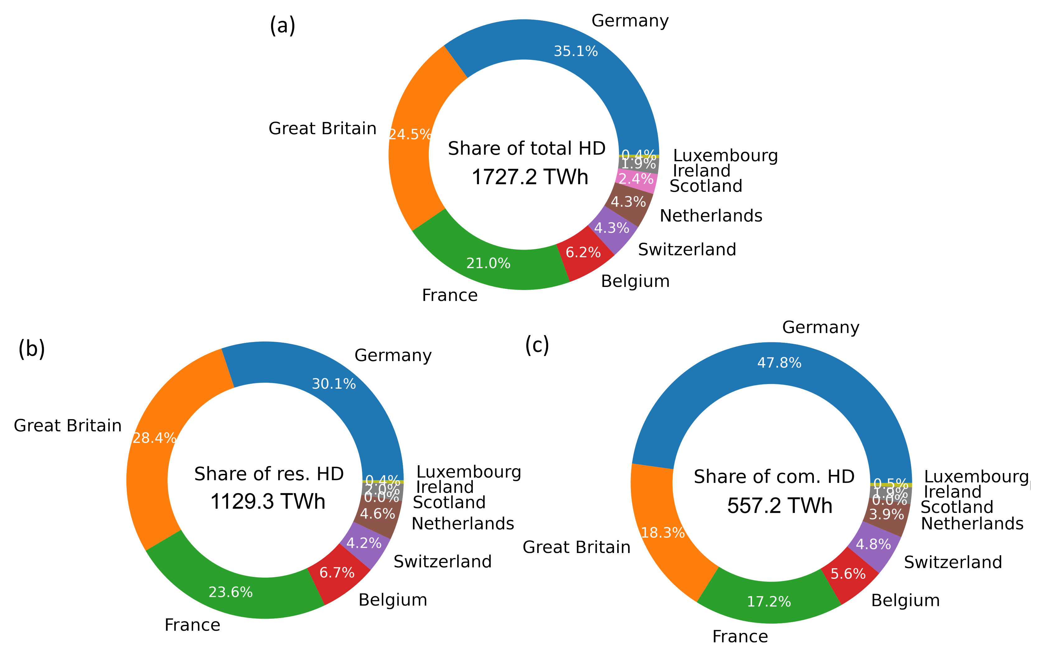
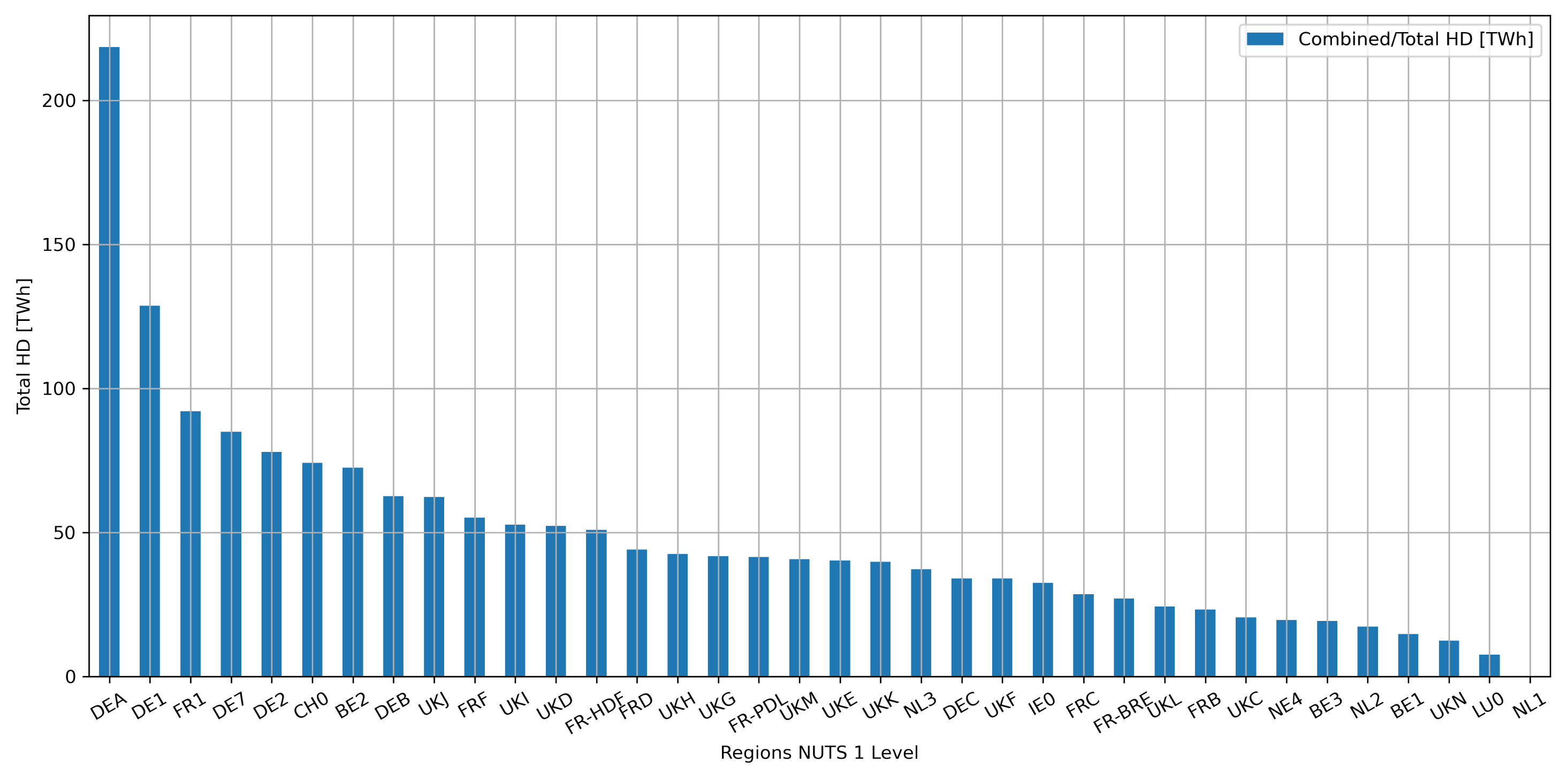
The statistical analysis reveals that only three countries (Germany, Great Britain, and France) account for ∼80% of the residential, commercial, and combined total heat demand while the remaining six countries account for ∼20% of the heat demand in the Interreg NWE region. The total heat demand covers only 16.1% of the entire Interreg NWE region. Apart from Germany, 2/3 to 3/4 of the total heat demand is attributed to the residential sector while 1/4 to 1/3 is attributed to the commercial sector. In Germany, the share of the commercial sector is noticeably higher (43.9%) and the residential heat demand is accordingly lower (56.1%). This discrepancy is associated with the fact that the Interreg NWE area for Germany covers the industrial centers in North Rhine Westphalia and in southern Germany with their associated commercial sectors adding disproportionately to the heat demand while more rural areas such as in northern and eastern Germany are not included in the calculations.

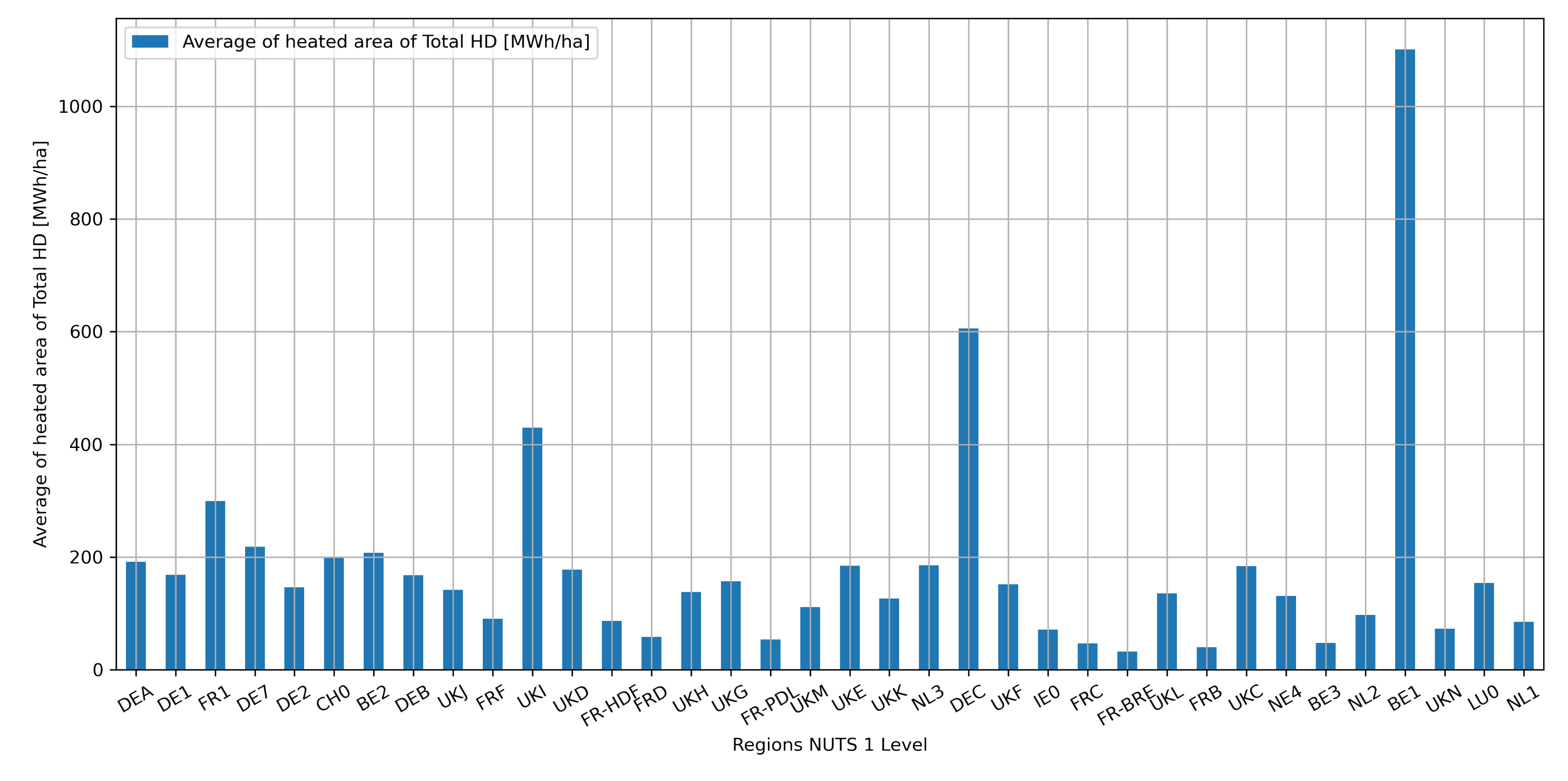
The average heat demand per heated area indicates that the heat demands are more decentralized in countries such as Switzerland, Germany, Great Britain, Luxembourg, the Netherlands, or Belgium (138.5 MWh/ha to 197.8 MWh/ha) while the spatial distributions of heat demands in countries like Ireland, Scotland and especially France (71.2 MWh/ha to 110.7 MWh/ha) are more centralized and limited to major cities. However, this calculation is biased as France represents 1/3 of the Interreg NWE region but only has the third-highest total heat demand. The same accounts for Ireland and Scotland with relatively large areas but also relatively low total heat demands. Furthermore, smaller countries like Luxembourg or Switzerland with alpine regions face different challenges discussed below.

4.2. Heat Demand Maps

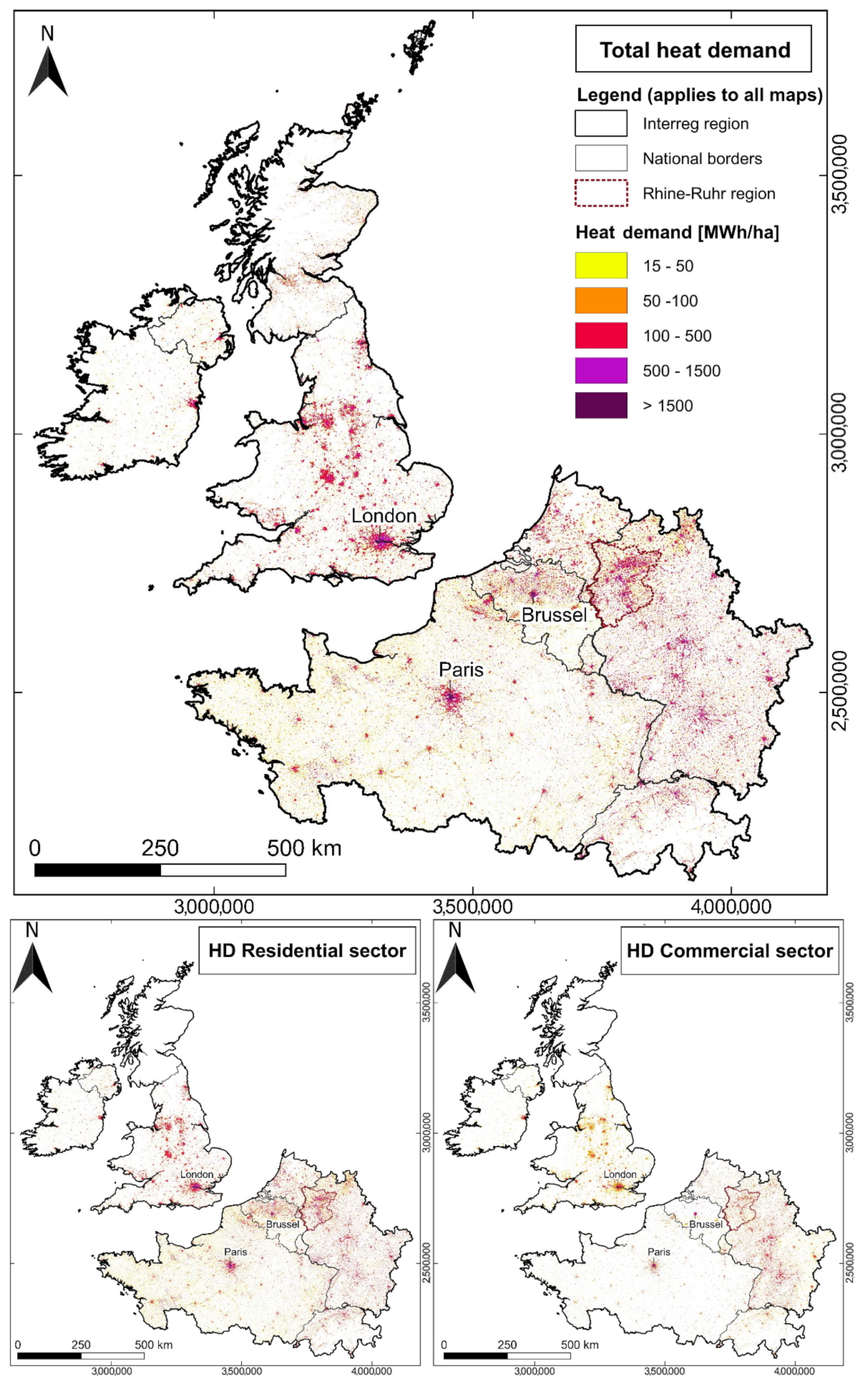
The regional disparities regarding HD distribution are explained by politics, topography, and the raw data. A clear indication for a climatic zone-related dependence on the HD, e.g., that more southern areas have to heat less, was not evident. The HD is usually clustered around economic centers. In more centralized countries, e.g., Great Britain or France, the HD has its highest value in the capital cities. This pattern is particularly apparent in countries with only one major economic center, e.g., Ireland or Luxembourg. This contrasts with more federal states like Germany, where the HD is evenly distributed across the country. The gradient in Belgium from the lowest HD values in the Walloon region to the highest in the Brussels area can only be explained to a limited extent with the previous assumption, e.g., the Ardennes are quite prominent in the southern parts, leading to a lower HD there. There is no evidence that the different input data types and methodologies for processing used in this study lead to a systematic over- or underestimation of HD. Border-sharp offsets in the HD calculation are more likely to occur due to the underlying data having different methodologies and assumptions.

A limiting factor of these maps is the age of the underlying raw data, which is sometimes older than 10 years and based on the EU Census 2011 or even previous periods. Since the census 2021 has been conducted recently, updated HD data and maps can be expected in the near future. Therefore, some countries are already in the process of updating their HD maps, with the older ones now being publicly unavailable. As a positive exception, up-to-date heat atlases have been provided by France. Another limitation is that much of the available HD data has still been calculated. The Netherlands should be mentioned here as a positive exception, which, although no official heat atlas exists, made large amounts of gas billing data anonymized and publicly available. However, one uncertainty remains concerning the efficiency of the gas-fired systems. Here, we introduced an efficiency factor $\eta$ that should be used for future calculations similar to factors for the efficiency of power networks as done by Ref. [52]. The aim to improve the existing HD maps from Hotmaps and HRE has thus only partially been achieved.

A majority of space heating and hot water is used for households and not for the commercial sector. The residential sector, therefore, predominates the HD maps primarily due to its quantity. The residential HD is spread throughout the countries with agglomerations in urban areas, while the commercial HD is predominantly concentrated in urban areas.

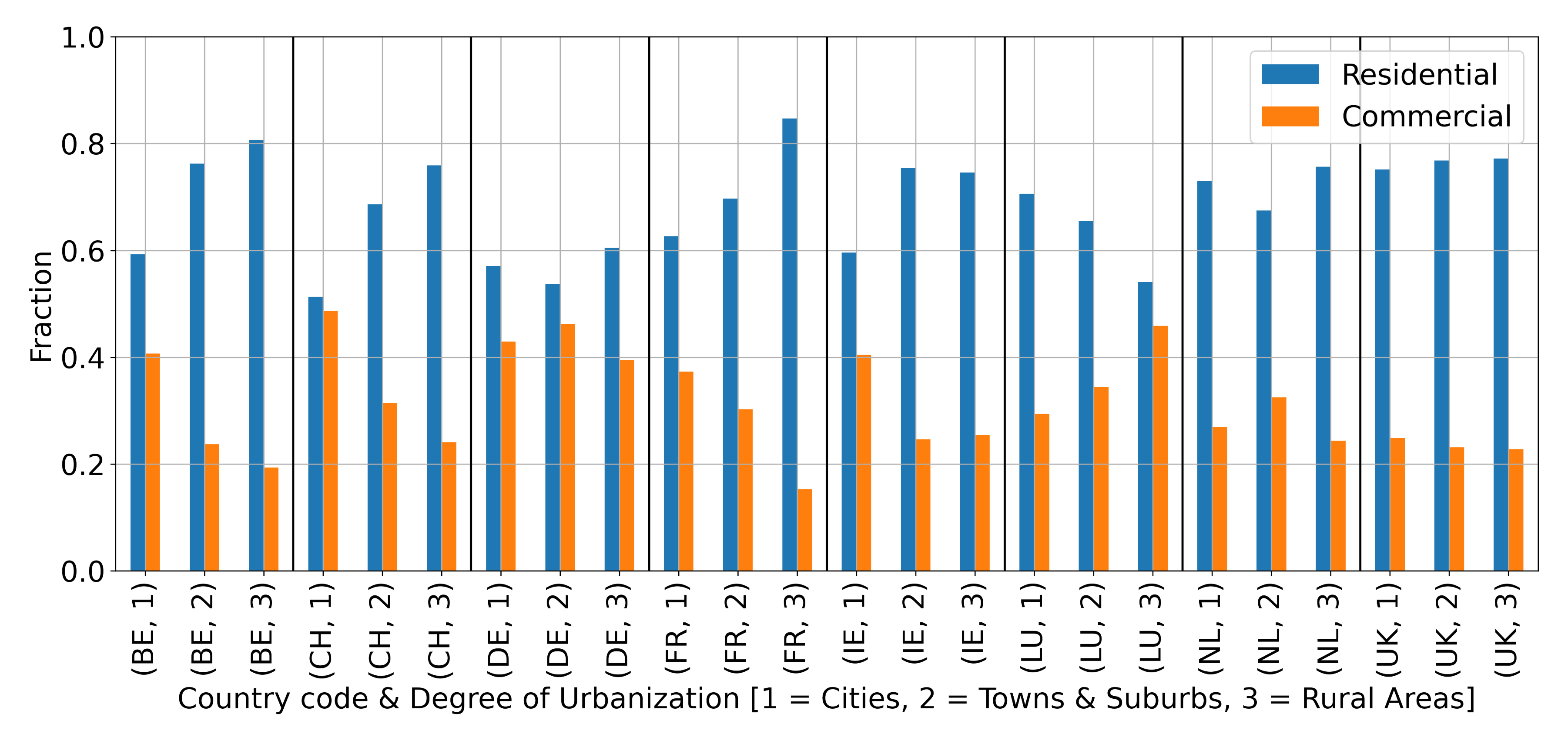
The share of the commercial sector increases with the degree of urbanization in most countries. The share of the commercial sector in Germany has a significantly higher level in all degrees of urbanization. This leads to the statement, that Germany has a highly developed commercial sector with a disproportionate high HD. An explanation for the reverse trends in Luxembourg may be the small area of the country with a large share of urban area. In the predominantly small settlements, there are not as many residential buildings for every commercially used building as in more urbanized areas. The small areas, in addition, cannot be compensated by larger settlements in rural areas.

The similar HD patterns of the residential map and the total HD maps can be explained by the high proportion of rural areas in the Interreg NWE region. The HD in the commercial sector is usually significantly lower than in the residential sector. Germany and the UK without SCT have a high commercial and residential HD, which explains the high share in the total HD. France, with predominantly rural areas, has the third highest HD because it has the largest proportion in the Interreg NWE area. The clusters with the highest HD are the most urbanized and therefore the areas with the highest population density.

Compared to energy statistics or electricity statistics, heat demand statistics are less accessible to the public. There are no official published HD values for the Interreg NWE region. A realistic conversion of national or European energy statistics to Interreg NWE HD values is beyond the scope of this work. The realistic spatial accuracy of the resulting maps is not the 100 m × 100 m shown. The reliability of the results at a resolution of 1 km × 1 km should be significantly higher since some of the underlying HD maps have been calculated from data with this resolution. In order to implement a local investment, e.g., implementation of a district heating network powered by geothermal energy, feasibility studies have to be carried out on-site. In addition, it should also be noted that industrial HD plays a decisive role if necessary.

Some regional data are also outdated or not available. Ireland, Switzerland, and parts of Germany (e.g., Hesse) have already announced to provide new heat demand data in the next years, which will highly improve the existing heat demand maps and can easily be integrated into the developed workflow. Including industrial heat demand data would be useful for a comprehensive mapping. For the evaluation of heat demand in the industrial sector on a regional to local scale, individual heat consumption data is required, which is publicly not available. Consortial projects on the decarbonization of heat in commercial areas could be one key driver for future data disclosure and implementation into heat demand maps.

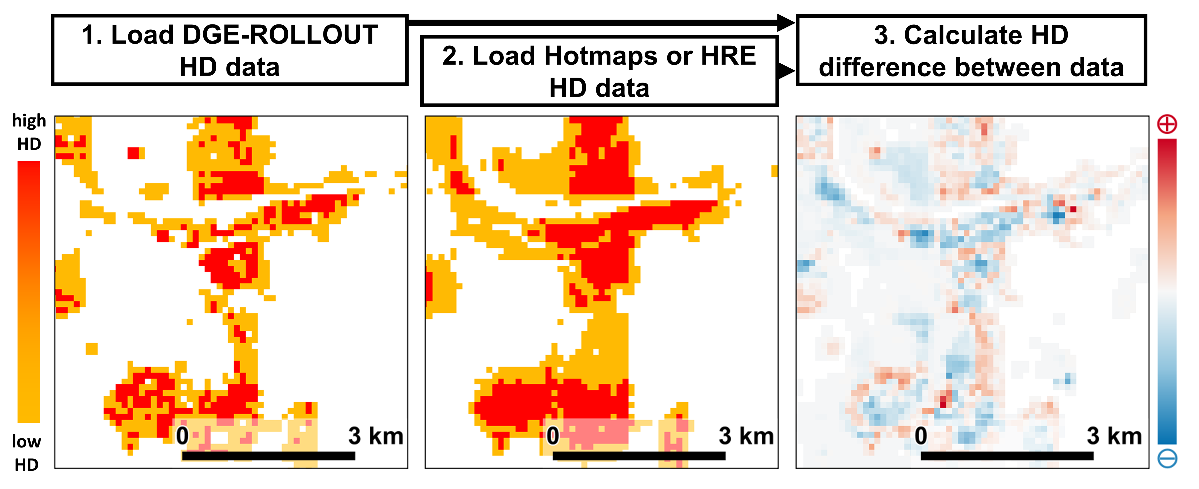
4.3. Heat Demand Difference Maps

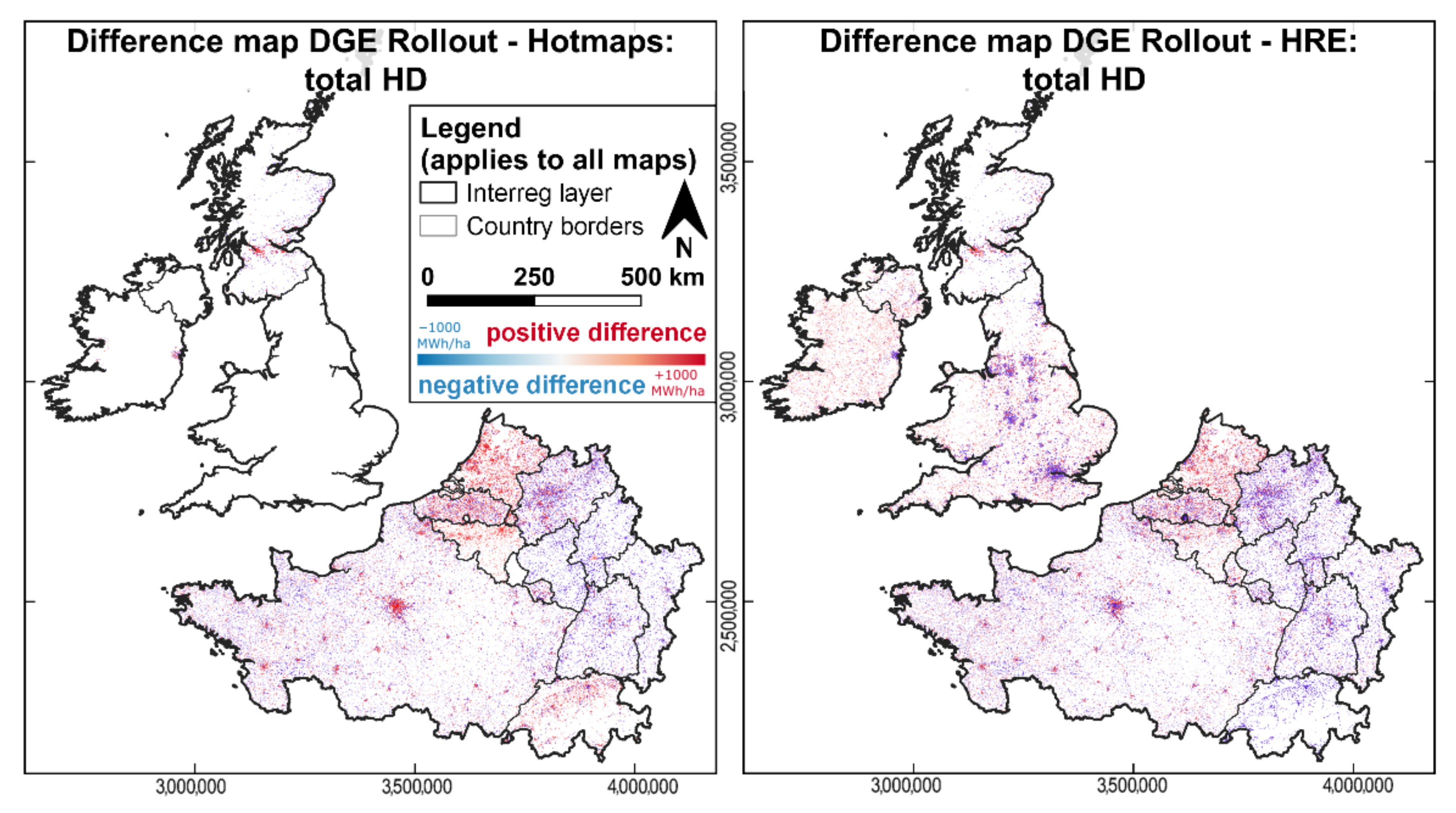
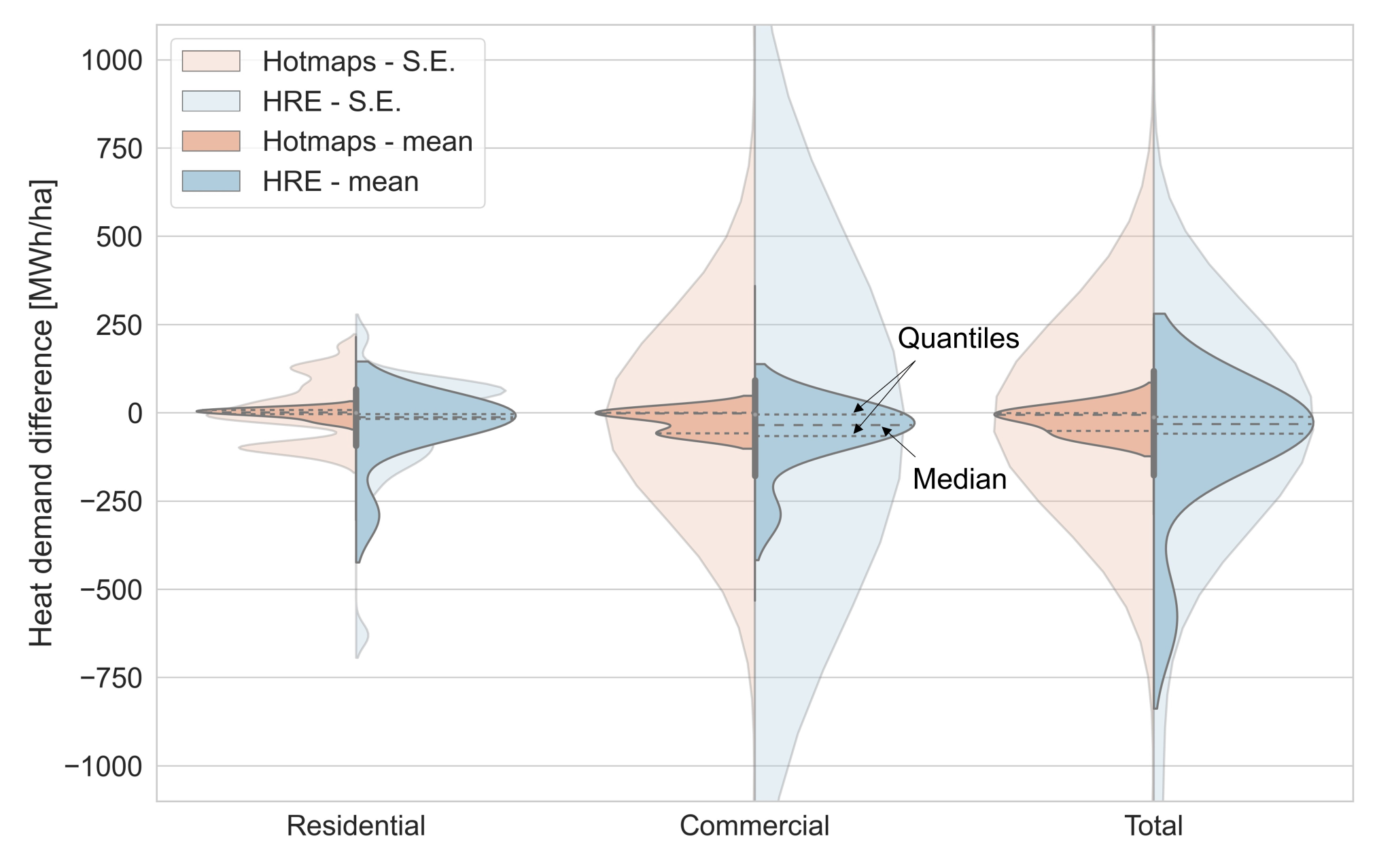
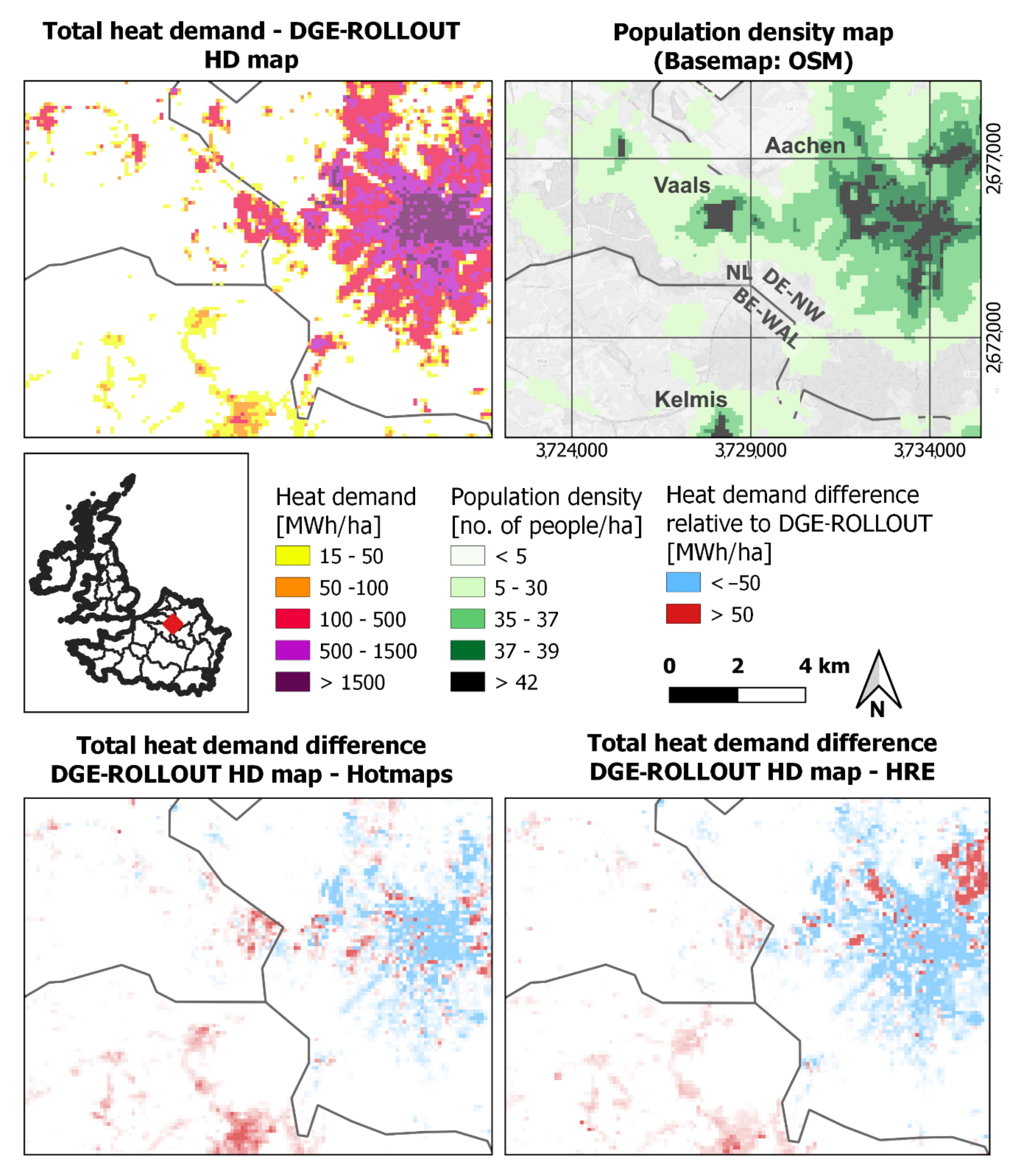
The deviations at the regional level can be explained by the underlying data. Regions based on the same dataset have a similar appearance in each HDDM, such as DE-RP and DE-HE. The Netherlands has low negative values in all HDDM. The conversion from gas demand data to HD data, based on the net calorific heating value of natural gas leads to a conservative calculation of the HD in the DGE-ROLLOUT map. The positive and negative deviations in the HDDM have the same order of magnitude. Thus, systematic errors can be neglected for the whole region. Strong negative HD differences around 100 m × 100 m for HDDM HRE commercial may indicate that there is a systematic underestimation of commercial HD in the DGE-ROLLOUT HD maps. The inversion from a positive HD difference inside conurbations to a negative difference in rural areas and vice versa could be caused by the insufficient use of uniform approaches for entire regions regardless of the local conditions. The exceptionally high differences of ±1000 MWh/ha for the city of Brussels (Belgium) HD in HDDM HRE can be explained with the underlying Hotmaps data. The city of Brussels area is highly urbanized and therefore, the HD tends to be overestimated. This leads to a positively biased median value since there are no rural areas, which would average out the overestimation of the result. Since Hotmaps data has been used to create several regional HD maps, the overall statistical dispersion is lower for Hotmaps than for HRE. The raw data of Scotland, residential and commercial, contains no HD data, and the HDDM for residential and commercial is therefore always negative. The spatial dispersion in the violin plots is based on a smoothed curve. With few values (16 mean and 32 standard error of mean values; for each region accordingly), outliers are very noticeable in the form of a second bulge or an abrupt end. An overall better prediction for the residential sector could be the reason for the irregularly shaped standard error of means curve. The low statistical dispersion of the mean values leads to a low statistical dispersion of positive and negative standard errors of the mean. Compared to Hotmaps and HRE, the HD in DGE-ROLLOUT tends to have slightly higher values since the averages are shifted into positive differences. The large dispersion for the commercial sector is a hint for a lower prediction quality of HD in this sector. In addition, there is an error propagation while summing up the residential and commercial sectors to the total sector, which leads to less accurate results for total HD compared to the residential sector HD.

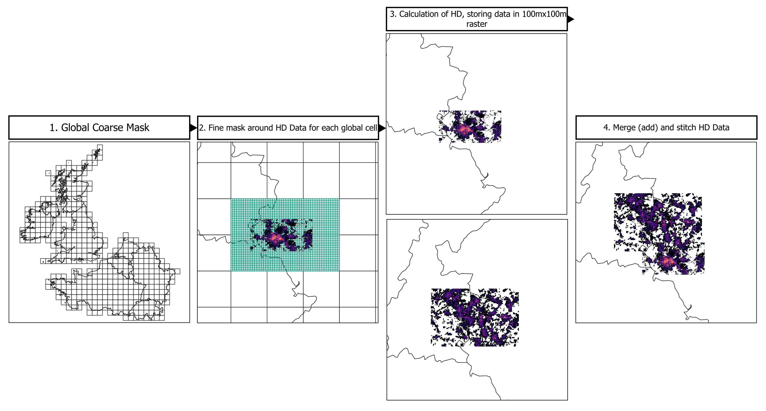
4.4. Computational Remarks

The computational time of processing entire states or NUTS regions such as North Rhine-Westphalia in Germany with its approximately 11 million building footprints may take up to 10 days. As this duration was deemed unfeasible, the R-tree [43] spatial index implemented in GeoPandas was utilized, which accelerated the processing of the North Rhine-Westphalia dataset by a factor of up to $1\times {10}^6$. To handle large state- to nationwide datasets, it is recommended to utilize the spatial index method implemented in PyHeatDemand [41]. This remarkable increase in computing performance also allows for a fast update once new heat demand input data becomes available or if other sources of heat need to be added.

5. Conclusions

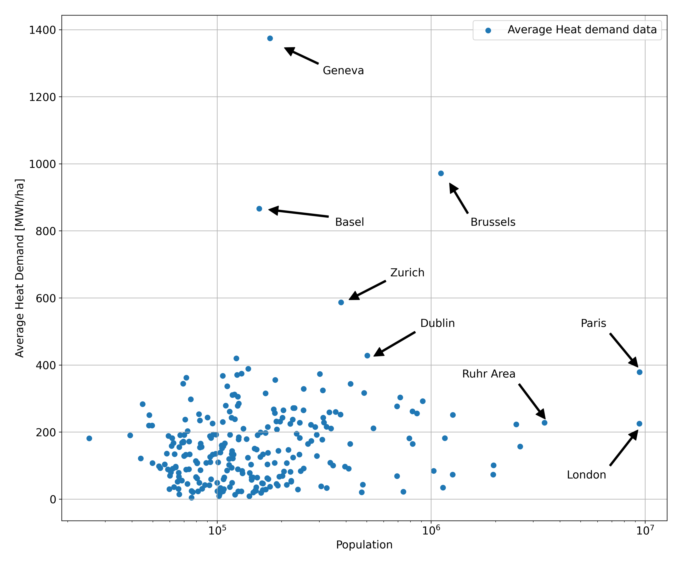
In this study, an efficient workflow for processing multi-type heat demand input data into multi-scale (local to transnational) harmonized heat demand maps is developed. The spatial distribution of the annual heat demand can be used to dimension large-scale heat pumps, for the heat demand planning of district heating systems, for communes according to the EU Energy Directive, or for geothermal applications. The methodology has been implemented in the open-source Python package PyHeatDemand, which makes it independent of geoinformation systems and guarantees reproducibility of the results. The implementation of spatial indices makes it a highly efficient tool where newly available heat demand data can easily be integrated at no time. The workflow was utilized for the development of three heat demand maps of the Interreg North-West-Europe region within the framework of the DGE-ROLLOUT project to demonstrate its applicability to transnational mapping tasks, which can also be performed on a regional to local level combining heat demands of, i.e., different cities. In the previous, data from various entities with different spatial resolutions and of different data formats have been integrated. The maps display the annual heat demand of the residential and commercial sectors and the sum of both sectors in the Interreg North-West-Europe region. The total heat demand of the Interreg North-West-Europe regions sums up to approximately 1700 TWh. The urban areas with the highest heat demand are the city of Paris (1400 MWh/ha), the city of Brussels (1300 MWh/ha), the London metropolitan area (520 MWh/ha), and the Rhine-Ruhr region (500 MWh/ha).

Heat demand difference maps allow statements about the plausibility of the results. With some outliers, especially in Germany and Belgium, the information value of the DGE-ROLLOUT maps is comparable with other projects on a European scale. The average total heat demand difference from the DGE-ROLLOUT maps to Hotmaps and HRE is 24 MWh/ha and 84 MWh/ha, respectively. Where heat demand needs to be calculated without metering data, different calculation models for cities and rural regions are recommended.

References

1. European Council; European Economic and Social Committee; Committee of the Regions. The European Green Deal. 2019. Available online: https://commission.europa.eu/strategy-and-policy/priorities-2019-2024/european-green-deal_en (accessed on 6 January 2024).
2. Reiter, U.; Catenazzi, G.; Jakob, M.; Naegeli, C. Mapping and Analyses of the Current and Future (2020–2030) Heating/Cooling Fuel Deployment (Fossil/Renewables)—Work Package 1: Final Energy Consumption for the Year 2012. 2016. Available online: https://energy.ec.europa.eu/publications/mapping-and-analyses-current-and-future-2020-2030-heatingcooling-fuel-deployment-fossilrenewables_en (accessed on 6 January 2024).
3. Technische Universität Wien; Fraunhofer ISI; Technical University of Denmark; OÖ Energiesparverband; IREES GmbH—Institut für Ressourceneffizienz und Energiestrategien; EE Energy Engineers GmbH; Gate 21; INEGI—Institute of Science and Innovation in Mechanical and Industrial Engineering; ABMEE—Agenția Pentru Managementul Energiei și Protecția Mediului; City of Litoměřice und Energy Cities France. Fostering the Use of Renewable Energies for Heating and Cooling (progRESsHEAT), 2014–2017. Available online: https://www.isi.fraunhofer.de/en/competence-center/energietechnologien-energiesysteme/projekte/317179_progressheat.html (accessed on 6 January 2024).
4. European Geothermal Energy Council. GeoDH—Geothermal District Heating, 2011–2014. Available online: http://geodh.eu/ (accessed on 6 January 2024).
5. Politechnika Krakowska. GRESHeat—Renewable Energy System for Residential Building Heating and Electricity Production. 2020. Available online: https://cordis.europa.eu/project/id/956255 (accessed on 10 January 2024).
6. Geological Survey of North Rhine-Westphalia; DMT Group; Energie Beheer Nederland B.V.; Flemish Institute for Technological Research; Fraunhofer IEG; French Geological Survey; Royal Belgian Institute for Natural Sciences; RWE Power AG; Technische Universität Darmstadt; Nederlandse Organisatie voor Toegepast Natuurwetenschappelijk Onderzoek. DGE-ROLLOUT—Roll-out of Deep Geothermal Energy in NWE, 2018–2022. Available online: https://www.nweurope.eu/projects/project-search/dge-rollout-roll-out-of-deep-geothermal-energy-in-nwe/ (accessed on 6 January 2024).
7. Salamon, M.; Thiel, A. Heißes Wasser aus der Erde. gdReport 2019, 2019, 4–7. Available online: https://www.gd.nrw.de/zip/gd_gdreport_1901s.pdf (accessed on 6 January 2024).
8. Fritschle, T.; Petitclerc, E.; van Melle, T.; Broothaers, M.; Passamonti, A.; Arndt, M.; Tasdemir, B.; Pederson, C.; Salamon, M. DGE-ROLLOUT: Promoting Deep Geothermal Energy in North-West Europe. 2021. Available online: https://www.geothermal-energy.org/pdf/IGAstandard/WGC/2020/40006.pdf (accessed on 6 January 2024).
9. Bracke, R.; Huenges, E.; Acksel, D.; Amann, F.; Bremer, J.; Bruhn, D.; Budt, M.; Bussmann, G.; Görke, J.; Grün, G.; et al. Roadmap Tiefe Geothermie für Deutschland—Handlungsempfehlungen für Politik, Wirtschaft und Wissenschaft für Eine Erfolgreiche Wärmewende—Strategiepaper von Sechs Einrichtungen der Fraunhofer Gesellschaft und der Helmholtz-Gemeinschaft. 2022. Available online: https://publica.fraunhofer.de/entities/publication/dc4a0733-2c1e-45ea-9600-0056ec82a0c0/details (accessed on 10 January 2024).
10. EU Parliament and Council. Directive 2012/27/EU of the European Parliament and of the Council. 2012. Available online: https://eur-lex.europa.eu/LexUriServ/LexUriServ.do?uri=OJ:L:2012:315:0001:0056:en:PDF (accessed on 6 January 2024).
11. Peeters, L. Warmte in Vlaanderen, Rapport 2020. 2021. Available online: https://www.vlaanderen.be/publicaties/warmte-in-vlaanderen-rapport-2020 (accessed on 6 January 2024).
12. Rohrbach, N. Thermische Netze: Nachfrage Wohn- und Dienstleistungsgebäude. 2020. Available online: https://www.bfe.admin.ch/bfe/de/home/versorgung/statistik-und-geodaten/geoinformation/geodaten/thermische-netze/waerme-und-kaeltenachfrage-wohn-und-dienstleistungsgebaeude.html#:~:text=Die%20W%C3%A4rmenachfrage%20von%20Wohn%2D%20und,%C2%B0C%20versorgt%20werden%20k%C3%B6nnen (accessed on 6 January 2024).
13. Landesanstalt für Umwelt Baden-Württemberg (LUBW). Methodologie der Wärmebedarfsdichte. 2017. Available online: https://www.energieatlas-bw.de/waerme/waermebedarf_wohnen/waermebedarfsdichte_von_wohngebaeuden (accessed on 6 January 2024).
14. Schmid, T. Dynamische und Kleinräumige Modellierung der Aktuellen und Zukünftigen Energienachfrage und Stromerzeugung aus Erneuerbaren Energien. PhD Thesis, Technical University of Munich, Munich, Germany, 2021. Available online: https://www.ffe.de/wp-content/uploads/2019/09/Dynamische-und-kleinraeumige-Modellierung-der-aktuellen-und-zukuenftigen-Energienachfrage-und-Stromerzeugung-aus-Erneuerbaren-Energien.pdf (accessed on 10 January 2024).
15. Koch, J. Informationen zu den Rahmendaten: Wärmebedarf, Energie-Atlas Bayern—Mischpult “Energiemix Bayern vor Ort”. 2020. Available online: https://www.energieatlas.bayern.de/kommunen/mischpult (accessed on 6 January 2024).
16. Landesamt für Natur, Umwelt und Verbraucherschutz Nordrhein-Westfalen. Methodologie Raumwärmebedarfsmodell NRW. 2021. Available online: https://www.opengeodata.nrw.de/produkte/umwelt_klima/klima/raumwaermebedarfsmodell/ (accessed on 6 January 2024).
17. Institut für ZukunftsEnergie- und Stoffstromsysteme. Wärmekataster Saarland. 2017. Available online: https://www.izes.de/de/projekte/w%C3%A4rmekataster-saarland (accessed on 6 January 2024).
18. Berry, M.; Melfort, C.; Potier, V. Cartographie des Besoins en Chaleur—Méthodologie de Calcul—Secteur Residentiel. 2020. Available online: https://reseaux-chaleur.cerema.fr/donnees-et-cartographies/carte-nationale-des-besoins-chaleur-secteur-residentiel-et-tertiaire (accessed on 6 January 2024).
19. Centraal Bureau voor De Statistiek (CBS). Woningen; Hoofdverwarmingsinstallaties, Wijken en Buurten. 2019. Available online: https://www.cbs.nl/nl-nl/cijfers/detail/85080NED (accessed on 6 January 2024).
20. Centraal Bureau voor De Statistiek (CBS). Elektriciteit en Warmte; Productie en Inzet Naar Energiedrager. 2019. Available online: https://www.cbs.nl/nl-nl/cijfers/detail/80030ned (accessed on 6 January 2024).
21. Ramboll A/S. Scotland Heat Map Public Sector Analysis. 2015. Available online: https://www.heatnetworksupport.scot/wp-content/uploads/2015/12/DistrictHeatingPublicSectorAnalysis.pdf (accessed on 6 January 2024).
22. Meha, M.; Novosel, T.; Duić, N. Bottom-up and top-down heat demand mapping methods for small municipalities, case Gllogoc. Energy 2020, 199, 117429. [Google Scholar] [CrossRef]
23. Aalborg University. Hotmaps—The Open Source Mapping and Planning Tool for Heating and Cooling, 2016–2020. Available online: https://www.hotmaps-project.eu/ (accessed on 6 January 2024).
24. Aalborg University. Heat Roadmap Europe 4. 2012. Available online: https://heatroadmap.eu/ (accessed on 6 January 2024).
25. Persson, U.; Möller, B.; Werner, S. Heat Roadmap Europe: Identifying strategic heat synergy regions. Energy Policy 2014, 74, 663–681. [Google Scholar] [CrossRef]
26. Hansen, K.; Connolly, D.; Lund, H.; Drysdale, D.; Thellufsen, J. Heat Roadmap Europe: Identifying the balance between saving heat and supplying heat. Energy 2016, 115, 1663–1671. [Google Scholar] [CrossRef]
27. Möller, B.; Wiechers, E.; Persson, U.; Grundahl, L.; Lund, R.; Mathiesen, B. Heat Roadmap Europe: Towards EU-Wide, local heat supply strategies. Energy 2019, 177, 554–564. [Google Scholar] [CrossRef]
28. Bertelsen, N.; Vad Mathiesen, B. EU-28 Residential Heat Supply and Consumption: Historical Development and Status. Energies 2020, 13, 1894. [Google Scholar] [CrossRef]
29. Nastasi, B.; Manfren, M.; Noussan, M. Open Data and Energy Analytics. Energies 2020, 13, 2334. [Google Scholar] [CrossRef]
30. Müller, A.; Hummel, M.; Kranzl, L.; Fallahnejad, M.; Büchele, R. Open Source Data for Gross Floor Area and Heat Demand Density on the Hectare Level for EU 28. Energies 2019, 12, 4789. [Google Scholar] [CrossRef]
31. Fry, N. Building-level heat demand mapping of commercial-residential areas for simulated district heating assessments in Montana, Idaho, and Washington. Energy Build. 2021, 245, 111075. [Google Scholar] [CrossRef]
32. Péter, C.; José, C.; Tamás, S.; Ádám, H.; Gábor, C.; Béla, M. Validation of Household Heat Demand in Rural Settlements using Software-Based Heat Atlases. In Proceedings of the International Conference of 3rd Smart Communities Academy, Legénd, Hungary, 15–16 April 2021; ISBN 9789634894285. Available online: https://m2.mtmt.hu/api/publication/32590389 (accessed on 10 January 2024).
33. Thomson, L.; Jenkins, D. The Use of Real Energy Consumption Data in Characterising Residential Energy Demand with an Inventory of UK Datasets. Energies 2023, 16, 6069. [Google Scholar] [CrossRef]
34. Vaisi, S.; Mohammadi, S.; Habibi, K. Heat Mapping, a Method for Enhancing the Sustainability of the Smart District Heat Networks. Energies 2021, 14, 5462. [Google Scholar] [CrossRef]
35. Novosel, T.; Pukšec, T.; Duić, N.; Domac, J. Heat demand mapping and district heating assessment in data-pour areas. Renew. Sustain. Energy Rev. 2020, 131, 109987. [Google Scholar] [CrossRef]
36. Schwanebeck, M.; Krüger, M.; Duttmann, R. Improving GIS-Based Heat Demand Modelling and Mapping for Residential Buildings with Census Data Sets at Regional and Sub-Regional Scales. Energies 2021, 14, 1029. [Google Scholar] [CrossRef]
37. Canet, A.; Qadrdan, M.; Jenkins, N. Heat demand mapping and assessment of heat supply options for local areas—The case study of Neath Port Talbot. Energy 2021, 217, 119298. [Google Scholar] [CrossRef]
38. Fesefeldt, M.; Capezzali, M.; Bozorg, M.; de Lapparent, M. Evaluation of future scenarios for gas distribution networks under hypothesis of decreasing heat demand in urban zones. Energy 2021, 231, 120909. [Google Scholar] [CrossRef]
39. Peronato, G.; Boghetti, R.; Kämpf, J. A machine-learning model for the prediction of aggregated building heating demand from pan-European land-use maps. J. Phys. Conf. Ser. 2021, 2042, 012019. [Google Scholar] [CrossRef]
40. Nishimwe, A.; Reiter, S. Estimation, analysis and mapping of electricity consumption of a regional building stock in a temperate climate in Europe. Energy Build. 2021, 253, 111535. [Google Scholar] [CrossRef]
41. Jüstel, A.; Strozyk, F. PyHeatDemand—Processing Tool for Heat Demand Data. J. Open Source Softw. 2024. in pre-review. Available online: https://github.com/openjournals/joss-reviews/issues/6041 (accessed on 6 January 2024).
42. Finkel, R.; Bentley, J. Quad trees a data structure for retrieval on composite keys. Acta Inform. 1974, 4, 1–9. [Google Scholar] [CrossRef]
43. Guttman, A. R-Trees: A Dynamic Index Structure for Spatial Searching. In Proceedings of the 1984 ACM SIGMOD International Conference on Management of Data, New York, NY, USA, 18–21 June 1984; pp. 47–57. [Google Scholar] [CrossRef]
44. QGIS Development Team. QGIS Geographic Information System. Open Source Geospatial Foundation. 2009. Available online: https://qgis.org/en/site/ (accessed on 6 January 2024).
45. Van Rossum, G.; Fred, L.D., Jr. The Python Language Reference Manual; Network Theory: New York, NY, USA, 1995; ISBN 978-1906966140. [Google Scholar]
46. Jordahl, K.; den Bossche, J.V.; Fleischmann, M.; Wasserman, J.; McBride, J.; Gerard, J.; Tratner, J.; Perry, M.; Badaracco, A.; Farmer, C.; et al. Geopandas: V0.8.1. 2020. Available online: https://zenodo.org/records/3946761 (accessed on 10 January 2024).
47. Gillies, S.; Shapely Developers. Shapely: Manipulation and Analysis of Geometric Objects. 2023. Available online: https://github.com/Toblerity/Shapely (accessed on 6 January 2024).
48. Gillies, S.; Rasterio Developers. Rasterio: Geospatial Raster I/O for Python Programmers. 2013. Available online: https://github.com/mapbox/rasterio (accessed on 6 January 2024).
49. Kluyver, T.; Ragan-Kelley, B.; Pérez, F.; Granger, B.; Bussonnier, M.; Frederic, J.; Kelley, K.; Hamrick, J.; Grout, J.; Corlay, S.; et al. Jupyter Notebooks—A publishing format for reproducible computational workflows. In Positioning and Power in Academic Publishing: Players, Agents and Agendas; Loizides, F., Schmidt, B., Eds.; IOS Press: Amsterdam, The Netherlands, 2016; pp. 87–90. [Google Scholar]
50. ISO/IEC 3166-1:2020; Codes for the Representation of Names of Countries and Their Subdivisions. International Organization for Standardization: Geneva, Switzerland, 2020; p. 31. Available online: https://www.iso.org/standard/72482.html (accessed on 6 January 2024).
51. Zijlema, P. The Netherlands: List of Fuels and Standard CO2 Emission Factors Version—Annual Update of Fuel List for the Netherlands. 2019. Available online: https://www.rvo.nl/sites/default/files/2023-08/The%20Netherlands%20list%20of%20fuels%20and%20standard%20CO2%20emission%20factors%20January%202022.pdf (accessed on 6 January 2024).
52. Majcen, D.; Itard, L.; Visscher, H. Theoretical vs. actual energy consumption of labeled dwellings in the Netherlands: Discrepancies and policy implications. Energy Policy 2013, 54, 125–136. [Google Scholar] [CrossRef]
53. Yang, X.; Hu, M.; Heeren, N.; Zhang, C.; Verhagen, T.; Tukker, A.; Steubing, B. A combined GIS-archetype approach to model residential space heating energy: A case study for the Netherlands including validation. Appl. Energy 2020, 280, 115953. [Google Scholar] [CrossRef]
54. Perry, M. Rasterstats. 2023. Available online: https://github.com/perrygeo/python-rasterstats (accessed on 6 January 2024).
55. The Pandas Development Team. Pandas. 2023. Available online: https://zenodo.org/records/10426137 (accessed on 10 January 2024).
56. Geoportal of the European Commission (Eurostat). GEOSTAT 1 km2 Population Grid. 2018. Available online: https://ec.europa.eu/eurostat/web/gisco/geodata/reference-data/population-distribution-demography/geostat (accessed on 7 January 2024).
57. Geoportal of the European Commission (Eurostat). DEGURBA—Degree of Urbanization: Population Distribution. 2020. Available online: https://ec.europa.eu/eurostat/web/gisco/geodata/reference-data/population-distribution-demography/degurba (accessed on 6 January 2024).
58. Maas, P.; Iyer, S.; Gros, A.; Park, W.; McGorman, L.; Nayak, C.; Dow, P. Facebook Population—Facebook Disaster Maps: Aggregate Insights for Crisis Response & Recovery. In Proceedings of the 16th ISCRAM Conference, València, Spain, 19–22 May 2019. [Google Scholar] [CrossRef]
Figure 1. Input and output data for top-down and bottom-up approaches. Note, that the resulting spatial resolution can be the same for both approaches, but the spatial value of information is usually lower using a top-down approach (after Ref. [22]).
Energies 17 00481 g001
Figure 2. Main steps from creating a coarse matrix to a fine matrix to calculating the final heat demand data.
Energies 17 00481 g002
Figure 3. Main steps of the methodology to process the provided HD polygons for the heat demand data categories 1 and 2.
Energies 17 00481 g003
Figure 4. Methodologies used for different heat demand input data. Top: Methodology used for heat demand categories 1, 2, and 4. For the methodology of heat demand category 3 (bottom), two input data types have been used: (a) the provided HD data with a low spatial resolution (point data per LAU) and (b) the Hotmaps data with a high spatial resolution (100 × 100 m 2 ). The calculated scaling factor has been used to rescale the Hotmaps data for the DGE-ROLLOUT HD map.
Energies 17 00481 g004
Figure 5. Interreg NWE region and the quality and spatial representation categories of each heat demand input data delivered by the responsible entities [40].
Energies 17 00481 g005
Figure 6. Main steps of developing the heat demand difference maps.
Energies 17 00481 g006
Figure 7. Heat demand in MWh/ha per year of the Interreg NWE region for the residential and commercial sector and both sectors summed up (total HD). The legend applies to all three maps. Scotland is not displayed in the residential or commercial heat demand maps since there is no data with subclassification for the different sectors available.
Energies 17 00481 g007
Figure 8. (a) Country share of the total Interreg NWE heat demand. Share of the residential (b) and commercial (c) heat demand per country.
Energies 17 00481 g008
Figure 9. Total Heat Demand [TWh] for the different NUTS-1 regions. Values are sorted by total HD.
Energies 17 00481 g009
Figure 10. Average of heated area of total HD [MWh/ha] for the different NUTS-1 regions. Values are sorted according to the total HD values shown in Figure 9.
Energies 17 00481 g010
Figure 11. Share of the residential and commercial sector in heat demand depending on the degree of urbanization in each country.
Energies 17 00481 g011
Figure 12. Ratios between population per city and summed up total heat demand per area definition according to the urban areas of the OECD.
Energies 17 00481 g012
Figure 13. Ratios between population per city and summed up total heat demand per hectare per area definition according to the urban areas of the OECD.
Energies 17 00481 g013
Figure 14. Series of HD difference maps, where the Hotmaps and HRE HD maps were subtracted from the DGE-ROLLOUT HD map for each raster cell in the residential, the commercial sector, and in total. For IR, the UK without SCT and LUX HD, data from Hotmaps has been used in the DGE-ROLLOUT HD map.
Energies 17 00481 g014
Figure 15. Violin plots showing the statistical dispersion of mean values for the residential sector, commercial sector, and for total HD difference with Hotmaps and HRE in comparison. The pale envelope in the background displays the statistical dispersion of the standard mean error.
Energies 17 00481 g015
Figure 16. DGE-ROLLOUT HD map of the city of Aachen and the three-country border between BE-WAL (data category 4), DE-NW (data category 1), and NL (data category 4). Note, that NL is based on real consumption data, whereas the other HD data are based on a modeled top-down approach.
Energies 17 00481 g016
Disclaimer/Publisher’s Note: The statements, opinions and data contained in all publications are solely those of the individual author(s) and contributor(s) and not of MDPI and/or the editor(s). MDPI and/or the editor(s) disclaim responsibility for any injury to people or property resulting from any ideas, methods, instructions or products referred to in the content.