Article

Optimal Control of Cascade Hydro Plants as a Prosumer-Oriented Distributed Energy Depot

by
Przemysław Ignaciuk
* and
Michał Morawski
Institute of Information Technology, Lodz University of Technology, Politechniki 8 St., 93-590 Łódź, Poland
*
Author to whom correspondence should be addressed.
Energies 2024, 17(2), 469; https://doi.org/10.3390/en17020469
Submission received: 16 December 2023 / Revised: 3 January 2024 / Accepted: 15 January 2024 / Published: 18 January 2024

Abstract

:
For political and economic reasons, renewable sources of energy have gained much importance in establishing a sustainable energy economy. By their very nature, however, their benefits depend on changeable weather conditions, and are unrelated to the generation and consumption patterns in industrial or home environments. This generation–dissipation disparity induces price fluctuations and threatens the stability of the supply system, yet can be alleviated by installing energy depots. While the classic methods of energy storage are hardly cost-effective, they may be supplemented, or replaced, by a distributed system of small-scale hydropower plants with ponds used as energy reservoirs. In this paper, following a rigorous mathematical argument, a dynamic model of a multi-cascade of hydropower plants is constructed, and a cost-optimal controller, with formally proven properties, is designed. On the one hand, it allows for an increase in the owners’ revenue by as much as 30% (compared to a free-flow state); on the other hand, it reduces the load fluctuation imposed on the grid and the legacy supply system. Moreover, the risk of floods and droughts downstream resulting from inappropriate use of the plants is averted.

1. Introduction

Energy demand grows day by day, including for home applications, industry, transportation, building cooling and heating, etc. Meanwhile, its price is increasing, hindering domestic budgets. For instance in Europe, tightening the restrictions on fossil fuels leaves renewable energy sources (RSEs): sun, wind, tidal, geothermal, and water flow [1], as the only viable options to decrease operational costs. Unfortunately, RSEs are ‘capricious’ in the sense that the amount of retrieved energy heavily relies on weather conditions, whereas the dissipation depends on human activities; both are unrelated to each other. These opposing factors lead to substantial price fluctuations and unpropitious variations of the grid load. In essence, an RSE generates inexpensive energy around noon, whereas the maximum demand (thus high prices) is in the evening when the costly fuel-sourced plants need to be engaged. As a result, the price variation can resemble the so-called ‘duck curve’, which is illustrated in Figure 1 for the first few days in July 2023 on the Polish energy market. On 2 July the price in the evening was over 40 times higher than at noon on that day (a sunny and windy Sunday with a lot of energy obtained from RSEs). Meanwhile, on 6 July, that ratio was less than 2 times more, and, overall, the prices were much higher. The increase of RSE-generated energy deepens the problem of imbalance and forces external control of micro-integrated energy systems [2] owned by prosumers. However, the surplus inexpensive energy may be used to supply the infrastructure or may be stored away, as is proposed in this work.
According to a common belief, electrical energy cannot be stored on a larger scale; i.e., its generation and dissipation must match. The differences emerge in frequency deviation, unless one finds a way to create energy depots or adjust the generation to temporary demands, which is possible but limited by technology. Therefore, significant emphasis is put on developing energy-storing solutions, encompassing pumped hydro plants, compressed air chambers, flywheels, and Saint Graal-hydrogen generation [3]. The idea presented here is intended to complement these solutions, rather than to replace them. It is directed at different markets—at citizens rather than industry.
Figure 1. Fluctuation of energy prices [PLN/MWh] on the Polish market in the first few days of July 2023 [4], following the ‘duck curve’.
Energies 17 00469 g001

1.1. Problem Context

The optimal scheduling of hydropower plant (HP) water release, commonly known as automatic generation control (AGC), has been investigated for quite some time ([5,6], and references therein). While the role the water plants play in flood/drought protection and power generation has been recognized, little attention has been devoted to another usage they may offer—energy storage reservoirs [7]. Instead of focusing just on the amount of generated electricity, a HP may be fine-tuned to regulate the water flow according to the time-varying demand and price profiles, thus acting as an energy depot or buffer. Consequently, what is proposed in this paper is to look at the HP also as an energy-storage system regulated in such a way that the water flow is throttled when the energy is cheap (usually at night and around noon) and released in the morning and evening when the energy is expensive. Such an application is economically advantageous to the traditional energy depots, compared with, e.g., pumped hydroelectric storage, or chemical batteries, which are costly to introduce (CAPEX) and maintain (OPEX). In fact, it is a win-win solution: the HP proprietor earns money benefitting from the price-fluctuation profile, and the grid operators and owners of the traditional plants “behead the duck” (flatten load variability) [8], decreasing operational expenditures. Also, as an ecological side effect, the soil-moisture level increases [9].

1.2. Literature Review

In this area of research, HPs are classified as normal HP (>100 MW), medium (<100 MW), small (<15 MW), mini (<1 MW), micro (<100 kW), and pico (<5 kW), where the actual values depend on the regional policy [10,11]. Most of the research conducted so far concerns small and large HPs as the primary suppliers of electricity. In contrast, in this work, owing to their function for prosumers, smaller installations—pico and micro—are given primary emphasis. The prospective model encompasses numerous formerly abandoned mills with small ponds (run-of-river HP) [12,13], which, when engaged, may significantly decrease capital expenditures. For instance, in Poland, currently fewer than 5% of such installations are used for energy production [14], thus the application area of the research presented here is meaningful. Obviously, a single prosumer depot does not provide sufficient input to be a game changer. However, as examined in this work, an optimally controlled set of interconnected prosumer HPs does. It will provide an efficient energy-storage system resistant to perturbations, with low installation and operational costs.
Micro [10] and pico [15] HPs are typically built as run-on-river installations [9,12], i.e., without large dams and reservoirs. Thus, the traditional control strategies developed as long-term (1–5 years), mid-term (3–18 months), and short-term (2–14 days) [3] are of little use here due to the limited volume of ponds. In the case of micro and pico HPs, a reasonable water accumulate–release scheduling strategy should be formulated for a time frame of a few hours, at most one day, and should be focused on decreasing the imbalance in the mornings and evenings (Figure 2). However, the constrained reservoir volume makes micro HPs vulnerable to temporary weather conditions. For example, a local storm can promptly fill up the pond near one HP, while, at the same time, a nearby station experiences intensified vaporization due to sunny weather. In the face of inaccurate precipitation forecasting and imprecise water runoff models, when the weather is unstable, AGC has to be recomputed frequently to adjust the system to the most recent conditions. It motivates the search for an optimal control solution that will capture the price and demand-profile characteristics, yet will not require frequent recalculations and changes in the dam control plan.
Actually, a similar idea—to engage prosumers in the propitious regulation of energy production and distribution—stands behind the popularity of photovoltaic (PV) installations, which have become a common element of the current energy manipulation landscape. However, there is a fundamental difference between PV and HP installations. The PV plants are mutually independent, while the operation of an HP relies on all the plants upstream, thus being more challenging to handle. A set of HPs utilizes the water that comes from the upstream flows and tributaries, with non-negligible delay, hence an improper AGC may destabilize the system and even trigger a flood. Therefore, it is mandatory to synchronize the HP operation, explicitly taking into account the distance between them, the predicted weather conditions, and specifics of the intended application—a distributed energy depot in addition to the typical function of power generation.
In the past, the scheduling of operation of a cascade of HPs has been investigated as a case study [16], rather than a control system, i.e., each plant is manually adjusted without enforcing a common framework. Other approaches reduce the HP cascade to a single-plant case [17], where dams are at a close distance [12,18], or located on one river but not on its tributaries [13,19]. All these models and control strategies do not fit into a prosumer system. The solution closest to the approach presented here has been recently delivered in [18]. However, it covers a dense cascade instead of a distributed networked system and is targeted to a different (frequency) market suitable for large HP installations for which short-term parameter variations, e.g., precipitation, do not impact the system dynamics.

1.3. Contribution

As noted in the preliminary study [20], in the research on the water-based energy systems, a major drawback is either placing too much emphasis on the theoretical aspects (and considering idealized scenarios to impose a given analytical framework) or, in contrast, focusing entirely on the practical issues, which leads to intricate, poorly formalized, often heuristic—thus untransferable—models and algorithms. Moreover, in the algorithm construction, the primary emphasis is given to reaching the desired state, not how it is achieved. Consequently, the models proposed for the considered class neglect many essential aspects related to the node dynamical interaction. In particular, the issues of delay in exchanging the resource—the water—among the reservoirs, and temporary conditions related to the uncertain intensity of precipitation, are omitted.
To capture the aforementioned objectives, the dynamical model constructed in this work includes information on the various delays in the water flows linking the reservoirs. Using the system’s dynamical representation, an optimization problem is formulated and solved analytically. The optimal control law is expressed in an easy-to-implement closed form, so it does not need frequent recomputation, as is the case in available numerical solutions. The proposed strategy brings profits not only to the prosumers by increasing their economic gain, but also to the power grid operators by reducing the load changes in the standard supply system.

1.4. Work Organization

The paper is organized in the following way. In Section 2, a discrete-time dynamic model of water flow in a multi-plant hydro system is constructed. It takes into account different plant characteristics, e.g., the conduit capacity and delays on the links between reservoirs. Based on the mathematical formulation of system dynamics, an optimization problem is defined and solved in Section 3. The system properties are discussed in Section 4. An illustration via a numerical example is provided. Conclusions are drawn in Section 5.

2. Materials and Methods

2.1. Modelling Strategy

Usually, the modeling of hydropower plants concentrates on the work of generators, and not the supply system [21,22]. However, in the proposed model, the generator is considered a black box, and the focus is placed on the water flow between the plants. A key point to consider in a water-reflow system is the non-negligible time between issuing the control action at one plant before it influences the water level at a downstream one. Therefore, as opposed to the earlier models of storage-distribution systems, e.g., [22,23], in the approach advocated here, the control principles from time-delay storage networks [24,25] will be applied. However, the model developed in [26] assumes continuous-time control adjustment, which is difficult to realize in a water-control system, owing to the specifics of the mechanical components steering the dam weirs. In turn, the discrete model considered in [26] does not include information about the price profile and weather forecast, vital for establishing an efficient usage plan in an energy storage network. The model proposed in this work explicitly incorporates the effects of finite sample time and delay and will be constructed directly in the discrete-time domain.

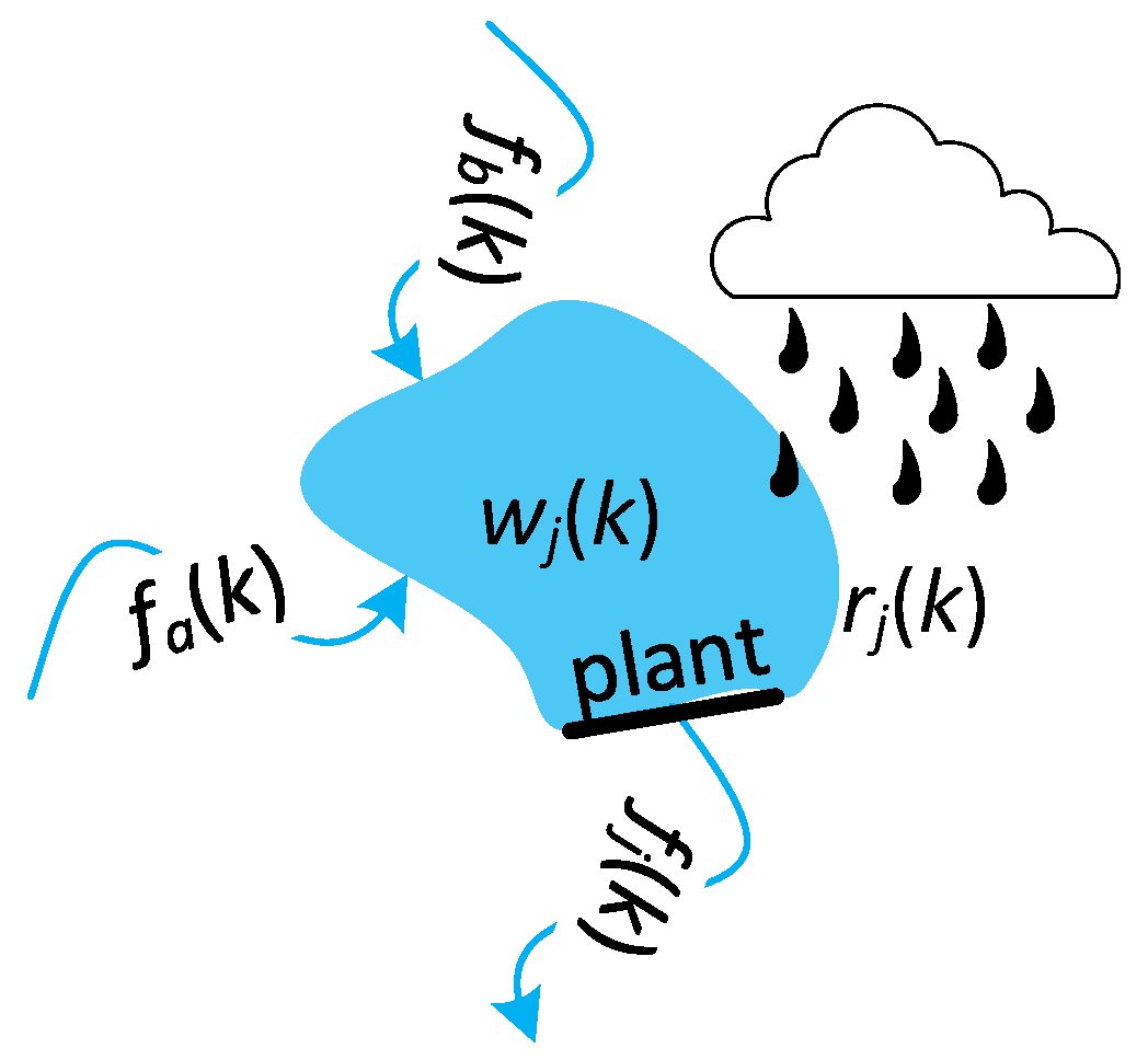
2.2. Plant-Reservoir Dynamics

Let us consider the model of a hydropower plant with a water-storage reservoir depicted in Figure 3. The water-budget dynamics at the plant may be described via the recurrence relation
w j ( k + 1 ) = w j ( k ) f j ( k ) + i p l a n t s u p s t r e a m f i ( k T i j ) + r j ( k ) ,
where
  • wj(k) is the water volume (equivalently the water level) in the reservoir,
  • fj(k) is the amount of water used to drive the plant power generators between time instants k and k + 1,
  • rj(k) is the supply from external hydrological sources like rain (and its runoff), melting snow, tributaries, vaporization, etc. The values of rj can be obtained from the weather forecast and hydrological models within the planning horizon of m periods, and rj(k) is assumed known, albeit time-varying. It may be positive, e.g., rain, or negative, e.g., vaporization, or soakage.
The tributaries supply the pond with the water previously used by the plants upstream. The water from upstream plant i arrives at plant j with Tij > 0 delay. The period length Δk, i.e., the time between instants k and k + 1, can be selected arbitrarily, but according to the pace of price changes, it is reasonable to choose 1 h (or 15 min when more accurate weather prediction models are accessible in the near future). Similarly, the planning horizon m usually covers a 24-h window of known energy prices (the next-day market), or a shorter one, as illustrated in Figure 2. The initial flow fj(k ≤ 0) and the initial water level wj(0) are assumed known.
The one-period income from the plant may be calculated as
J j ( k ) = η j p ( k ) f j ( k ) Δ k ,
where:
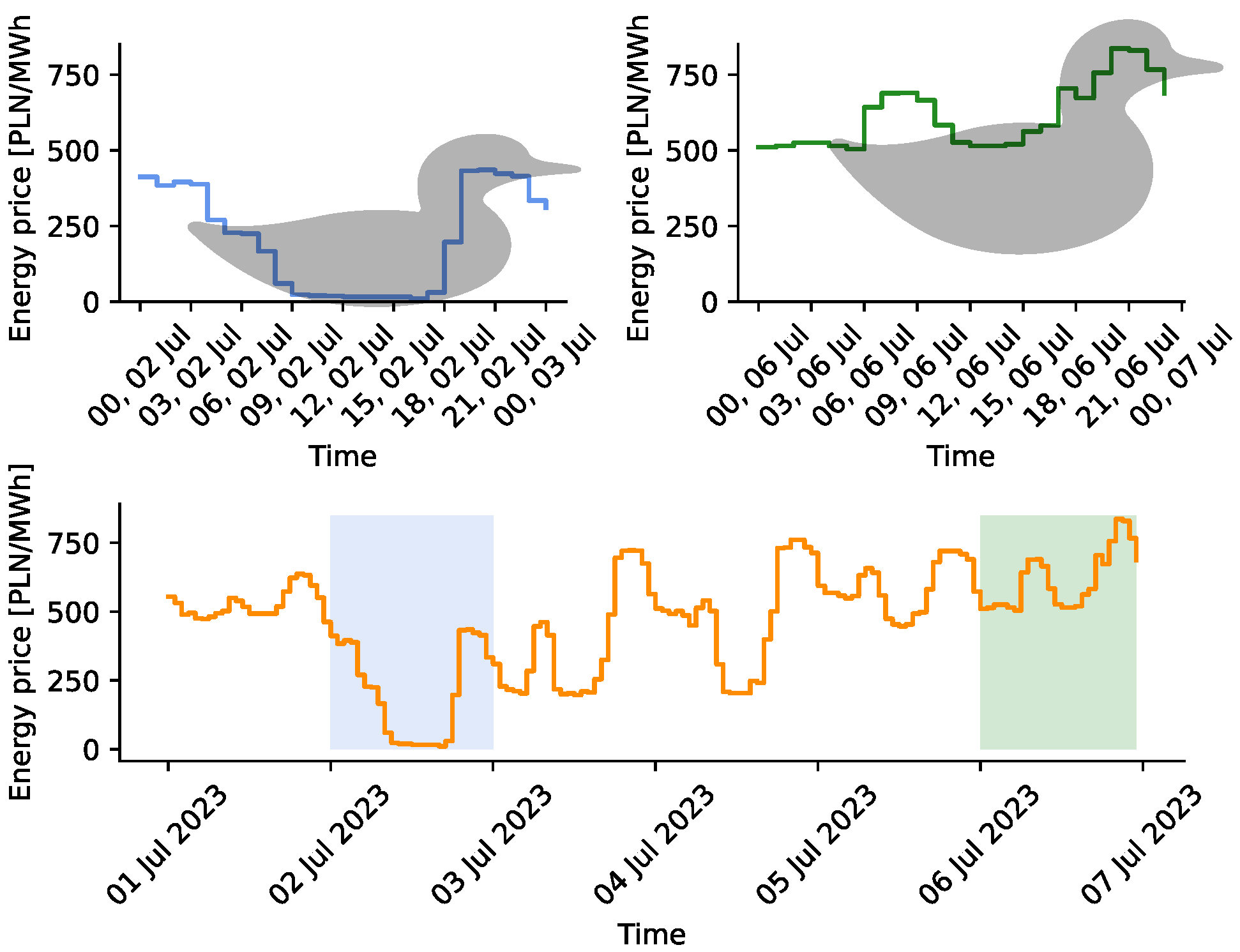
  • p(k) is the energy price at instant k, reflecting the duck curve, possibly moderated according to the specific local demands or tariffs;
  • ηj is the efficiency of power generators, including the impact of the dam height. For prosumer generators in the lowlands, the flow of 1 m3/s corresponds to the power generation of 5–7 kW per unit of the dam height.

2.3. Cascade Multi-Plant System

In the case of n power plants under common management (an example system with four plants illustrated in Figure 4), it is convenient to describe the model in a vector form with []’ denoting transposition. Let:
  • x(k) = [x1(k) x2(k) … xn(k)]’ be the vector of controlled flows: x(k) = f(k) − fref, where fref is the vector of natural flows;
  • s(k) = [s1(k) s2(k) … sn(k)]’ be the vector of water volume in reservoirs 1…n corresponding to controlled flows x1xn;
  • r(k) = [r1(k) r2(k) … rn(k)]’ be the water volume from exogenous sources.
Using this notation, the state–state representation of system dynamics may be written as
s ( k + 1 ) = s ( k ) + t = 0 T Θ t x ( k t ) + r ( k ) ,
where T is the maximum delay. Matrix Θ0 = −I, I is an n × n identity matrix, whereas Θ1ΘT group the information about the flow delays,
Θ t = θ i j n × n ,
with θij = 1, if the flow from reservoir j reaches reservoir i with delay t, and 0, if otherwise. The entries on the main diagonal θii = 0. Contrary to [18], here the distance between the plants is non-negligible. For the example in Figure 4, the flow between reservoirs 1 and 3 has the longest delay, thus T = 3. The system structural matrices in that case are:
Θ 1 = 0 0 0 0 0 0 0 0 0 0 0 0 0 0 1 0 , Θ 2 = 0 0 0 0 0 0 0 0 0 1 0 0 0 0 0 0 , Θ 3 = 0 0 0 0 0 0 0 0 1 0 0 0 0 0 0 0 .
For the convenience of further analysis, two auxiliary matrices will be introduced:
Θ ̆ = t = 1 T Θ t ,
and
Θ = t = 0 T Θ t = Θ ̆ I .
Using (1) and (3), the vector of water levels in the reservoirs w(k) = [w1(k) w2(k) … wn(k)]’ can be related to the controlled volume as
w ( k ) = s ( k ) + i = 0 k 1 Θ f r e f = s ( k ) + k Θ f r e f .

3. Results

3.1. Problem Formulation

Taking the initial level as s(0) and the initial flow as x(k ≤ 0) = 0, the task is to reach level s(m) within m periods so that the imposed cost criteria are fulfilled. Formally, the optimization problem may be stated as
max x ( k ) J E ( p ( k ) , x ( k ) ) = 1 2 k = 0 m 1 p ( k ) x ( k ) N x ( k ) ,
subject to (3), where N = diag{η1, η2, …, ηn} is a positive definite matrix of weighting coefficients that correspond to the efficiency of energy conversion at the plants.

3.2. Preliminaries

Before solving problem (8), a few properties of the proposed model will be defined and proved.
Lemma 1.
Matrix Θ ̆  is nilpotent with index n.
Proof. 
Without loss of generality, the reservoirs may be numbered according to the number of output conduits. Then, since the graph is directed, and the connections between the neighboring reservoirs are unidirectional (θij 0 ⇒ θji = 0), Θ ̆ takes the form of a strictly lower triangular matrix,
Θ ̆ = 0 0 0 0 θ 21 0 0 0 θ 31 θ 32 0 0 θ n 1 θ n 2 θ n , n 1 0 .
Some entries of Θ ̆ may be null: θij = 0 when there is no connection between reservoirs i and j. ☐
The characteristic polynomial of Θ ̆ ,
P ( γ ) = det ( γ I Θ ̆ ) = ( γ γ 1 ) ( γ γ 2 ) ( γ γ n ) ,
where γ1γn are the eigenvalues. In the case of matrix (9), all the eigenvalues γ1 = γ2 = … = γn = 0 and
p ( λ ) = λ n .
By the Cayley-Hamilton theorem, a matrix satisfies its characteristic polynomial,
P ( Θ ̆ ) = Θ ̆ n = 0 ,
so Θ ̆ is nilpotent with index n.
Lemma 2.
The inverse of “−Θ” is a positive matrix.
Proof. 
It is required to show that the entries of −Θ−1 are all non-negative. First, it will be demonstrated that −Θ is invertible. Using the same concept as in the organization of the entries of matrix (9), Θ takes the form of a lower triangular matrix with “−1” on the main diagonal:
Θ = 1 0 0 0 θ 21 1 0 0 θ 31 θ 32 1 0 θ n 1 θ n 2 θ n , n 1 1 .
The determinant of Θ,
det ( Θ ) = ( 1 ) n ,
so Θ has an inverse. Next, consider the power series
I + Θ ̆ + Θ ̆ 2 + ,  
and the partial sum
S k = I + Θ ̆ + Θ ̆ 2 + + Θ ̆ k
for some integer k. Note that
( I Θ ̆ ) S k = I Θ ̆ k + 1 .
When Θ ̆ k+10, then Sk → (I Θ ̆ )1. Therefore, since Θ ̆ is nilpotent (Lemma 1), series (15) converges, and the inverse of −Θ can be written as
Θ 1 = ( I + Θ ̆ ) 1 = ( I Θ ̆ ) 1 = I + Θ ̆ + Θ ̆ 2 + + Θ ̆ k 1 .
Since all the entries of Θ ̆ are non-negative, according to (18), so are the entries of −Θ−1. −Θ−1 is thus a positive matrix.
The considered problem is difficult to treat analytically owing to the delays in the water reflow. For that reason, an alternative, equivalent system description will be used. Let y(t) denote the overall system resource level, i.e., the sum of water volume accommodated in the reservoirs, and the water flowing between them subjected to control x,
y ( k ) = s ( k ) + j = 1 T t = j T Θ t x ( k t ) .
Lemma 3.
The dynamics of y(t) can be described by
y ( k + 1 ) = y ( k ) + Θ x ( k ) + r ( k ) .
Proof. 
Directly from the definition of y, under zero initial input, y(0) = s(0). Thus, applying (3) to (20), one has
y ( 1 ) = s ( 1 ) + j = 1 T t = j T Θ t x ( 1 t ) = s ( 0 ) + 0 + t = 1 T Θ t x ( 0 ) + r ( 0 ) = s ( 0 ) + Θ x ( 0 ) + r ( 0 ) .
Therefore, (20) is satisfied at k = 0. Afterwards, for any period k > 0, the following relation can be established:
y ( k + 1 ) = s ( k + 1 ) + j = 1 T t = j T Θ t x ( k + 1 j ) = s ( k ) + t = 0 T Θ t x ( k t ) + r ( k ) + j = 1 T t = j T Θ t x ( k + 1 j ) = s ( k ) + Θ 0 x ( k ) + Θ 1 x ( k 1 ) + + Θ T x ( k T ) + r ( k ) + Θ 1 + + Θ T x ( k ) + Θ 2 + + Θ T x ( k 1 ) + + Θ T x ( k T + 1 ) = s ( k ) + Θ 1 + + Θ T x ( k 1 ) + Θ 2 + + Θ T x ( k 2 ) + + Θ T 1 + Θ T x ( k T + 1 ) + Θ T x ( k T ) + Θ 0 + + Θ T x ( k ) + r ( k ) = s ( k ) + j = 1 T t = j T Θ t x ( k j ) + Θ x ( k ) + r ( k ) = y ( k ) + Θ x ( k ) + r ( k ) .
Using the principle of mathematical induction, one may conclude that the lemma holds for any k ≥ 0.
Theorem 1.
The optimization problem with functional (8) under constraint (20) is convex.
Proof. 
An optimization problem is convex when both the objective function and all the constraints are convex. ☐
A power function ()ε on R++ (positive real numbers) is convex if the exponent ε ≤ 0 or ε ≥ 1. All the linear functions are convex, too. Since both the cost functional (8) and system constraint (20) are convex, the considered optimization problem is convex.
Using the information provided by Lemmas 1–3 and Theorem 1, we are ready to approach the solution of the problem (8).

3.3. Solution

For the performance index in problem (8), the Hamiltonian can be defined as
H ( k ) = 1 2 p ( k ) x ( k ) N x ( k ) + λ ( k + 1 ) y ( k ) + Θ x ( k ) + r ( k ) ,
where λ′(t + 1) is a row vector of Lagrange multipliers.
The necessary conditions are as follows:
  • state equation
    y ( k + 1 ) = H ( k ) λ ( k + 1 ) = y ( k ) + Θ x ( k ) + r ( k ) ,
  • costate equation
    λ ( k ) = H ( k ) y ( k ) = λ ( k + 1 ) ,  
  • stationarity condition
    0 = H ( k ) x ( k ) = 1 2 p ( k ) N + N x ( k ) + Θ λ ( k + 1 ) = p ( k ) N x ( k ) + Θ λ ( k + 1 ) .
Solving (26) for x, yields
x ( k ) = p 1 ( k ) N 1 Θ λ ( k + 1 ) .
Note that since N is positive definite (a diagonal matrix with all positive entries), its inverse does exist.
Then, substituting (27) into (24) gives
y ( k + 1 ) = y ( k ) p 1 ( k ) Θ N 1 Θ λ ( k + 1 ) + r ( k ) .
Equation (25) is a homogeneous difference equation. Its solution with the terminal condition λ(m) is
λ ( k ) = λ ( m ) .
Substituting (29) into (28), yields
y ( k + 1 ) = y ( k ) p 1 ( k ) Θ N 1 Θ λ ( m ) + r ( k ) .
With the initial resource level y(0) the solution of (30) is
y ( k ) = y ( 0 ) + i = 0 k 1 r ( i ) p 1 ( i ) Θ N 1 Θ λ ( m ) .
The initial state y(0) and the final state y(m) are fixed, so their first derivatives are equal to zero. Using (31), the final resource level may be calculated as
y ( m ) = y ( 0 ) + i = 0 m 1 r ( i ) p 1 ( i ) Θ N 1 Θ λ ( m ) .
Hence, the terminal value of the Lagrange multiplier vector
λ ( m ) = Θ N 1 Θ 1 y ( m ) y ( 0 ) i = 0 m 1 r ( i ) / i = 0 m 1 p 1 ( i ) ,
and, using (29),
λ ( k ) = λ ( m ) = Θ N 1 Θ 1 y ( m ) y ( 0 ) i = 0 m 1 r ( i ) i = 0 m 1 p 1 ( i ) .
Note that since ΘN−1Θ′ is symmetric and N−1 = diag{η1−1, η2−1, …, ηn−1} positive definite, ΘN−1Θ′ is positive definite, thus invertible.
Using (27) and (34), the optimal control
x ( k ) = p 1 ( k ) N 1 Θ λ ( k + 1 ) = p 1 ( k ) N 1 Θ Θ N 1 Θ 1 y ( m ) y ( 0 ) i = 0 m 1 r ( i ) i = 0 m 1 p 1 ( i ) .
Since Θ is invertible and N−1 is a diagonal matrix with non-zero entries,
N 1 Θ Θ N 1 Θ 1 = N 1 Θ N 1 Θ 1 Θ 1 = Θ 1 .
Therefore, (35) simplifies to
x ( k ) = p 1 ( k ) Θ 1 y ( m ) y ( 0 ) i = 0 m 1 r ( i ) / i = 0 m 1 p 1 ( i ) .
It follows from (19) that
y ( m ) = s ( m ) + j = 1 T t = j T Θ t x ( m t ) ,
so the control system is noncausal. However, when m » T, then y(m) ≅ s(m), which results in the following causal control law
x ( k ) p 1 ( k ) i = 0 m 1 p 1 ( i ) Θ 1 s ( m ) s ( 0 ) i = 0 m 1 r ( i )
to be applied in system (3). This conclusion completes the solution procedure.
The obtained control law is amenable to physical interpretation and can be directly and efficiently implemented in dam control systems. Its properties are discussed in the next section.

4. Discussion

4.1. System Properties

Looking at how the flow control signal in (39) is established, a few observations can be made:
P1:
The current flow value depends on the current price, yet not on the water level. Thus, the prone-to-error water level measurements are not needed for the control law implementation.
P2:
Since −Θ is a positive matrix and the price is also positive, the flow control signal does not change the sign in the entire planning horizon. It either reduces the water inflow in the case of heavy rainfall and a risk of flood, or magnifies the flow intensity for the prosumers to gain more profit.
P3:
The flow intensity does not depend on the temporary rainfall intensity, but on its cumulative value i = 0 m 1 r ( i ) , which implies a certain degree of robustness to weather-condition fluctuations. The control system is resistant to temporary changes of opposite polarity.
P4:
With
K = Θ 1 i = 0 m 1 p 1 ( i ) s ( m ) s ( 0 ) i = 0 m 1 r ( i ) ,
substituting (39) for x(k) in (3), one obtains
s ( k + 1 ) = s ( k ) + t = 0 T Θ t p 1 ( k t ) K + r ( k ) .
Therefore, the closed-loop system with control (39) maintains the integrating property. For any k, one has
s ( k ) = s ( 0 ) + i = 0 m 1 t = 0 T Θ t p 1 ( i t ) K + i = 0 m 1 r ( i ) .
P5:
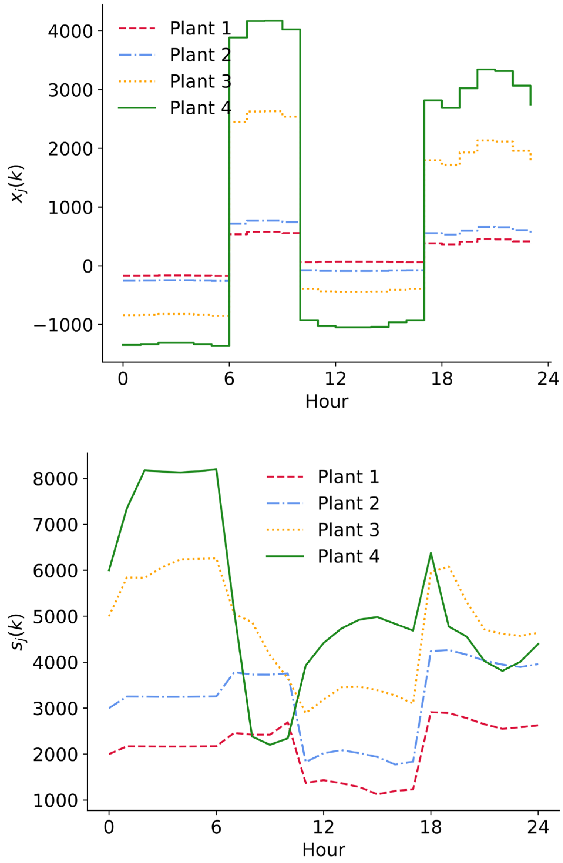
The water level exhibits neither oscillations nor overshoots. It is confined to the interval determined by the initial s(0) and terminal value s(m).

4.2. Practical Considerations

In a physical system, the variables may encounter physical constraints:
f j min f j ( k ) f j max , x j min x j ( k ) x j max , s j min s j ( k ) s j max ,
related to the conduit and reservoir capacity. Control (39) entering the saturation region (43) is no longer optimal. In such a case, the optimal values of x(k) can be obtained from numerical procedures, like those proposed in [3,18,27,28,29,30,31,32]. However, in the analyzed class of systems—networked systems with non-negligible time delays—the majority of classic numerical algorithms are not robust, even in relatively simple cases [32]. Moreover, the computations of AGC take a long time, which is rarely available due to weather fluctuations.
Therefore, in a practical setting, the control sequence is determined in a three-stage procedure:
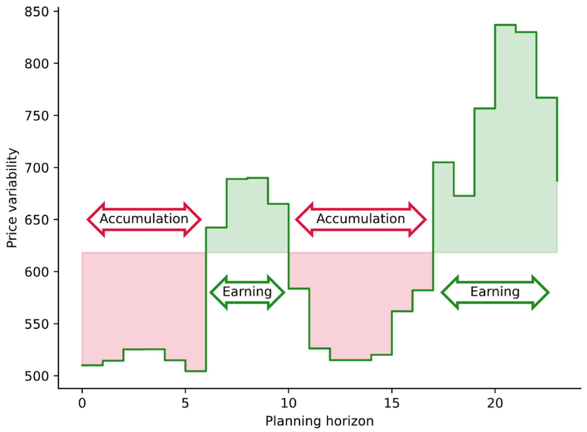
  • Within the planning horizon, identify zones of ‘accumulation’ (when the energy price is below the average) and ‘earning’ (when the energy price is above the average), as illustrated in Figure 2.
  • For each zone, calculate x(k) according to the closed-form expression (39), which is computationally not involving.
  • Use the solution obtained in Step 2 as an initial value (the initial guess) for the numerical algorithm to determine the optimal sequence in the presence of hard constraints (43).
Using the optimal control (39) as a starting point for a numerical algorithm relieves the computational burden and improves computational stability.

4.3. Numerical Example

In order to verify the analytical considerations from the previous sections, a series of tests for the topology in Figure 4 and the price profile in Figure 1, 6 July, has been conducted. In contrast to the common simplifications of a linear cascade encountered in the current literature, the chosen topology has a tree-like shape with the root at the river influx and branch tributaries. Hence, it reflects more closely the real environments in the considered application area, yet is simple enough to illustrate the control-system properties.
The system is supplied with the precipitation and corresponding runoff depicted in Figure 5. The simulation parameters are set as:
  • the initial water level in the reservoirs: s(0) = [2, 3, 5, 6]′ × 103 [m3],
  • the desired final water level: either s(m) = [1, 1.5, 2.5, 3]′ × 103 [m3], or s(m) = [3, 4.5, 7.5, 9]′ × 103 [m3], depending on the accumulation/earning period (Figure 2),
  • the natural flow fref = [1, 1.5, 2.5, 3]′ × 103 [m3/h].
The optimal control sequence x(k) calculated according to (39) and water-level evolution s(k) is sketched in Figure 6. The prosumer gain for a typical workday (6 July), and RSE-reach Sunday (2 July) from Figure 1 are displayed in Table 1.
In the considered example, one observes both the accumulation of energy in the reservoirs and water release (earning). Each plant in the linked cascades 1–3–4 and 2–3–4 either throttles or magnifies the flow intensity depending on how far it is located down the river, which is intuitively justified. However, while the reservoir occupancy s(k) for the first HPs (plants 1 and 2) in the cascades is a direct integral of x(k), the further down the river, the more profound the effect of the upstream HPs and delays. x(k) and s(k) fluctuate in the opposite direction according to the external excitation in the ‘accumulation’ and ‘earning’ periods, as shown in Figure 6 (see also Figure 2). Although s3(k) and s4(k) differ much in shape from s1(k) and s2(k), they satisfy property P4, i.e., for each j, s j min s j ( k ) s j max , with no oscillations within each accumulation/earning period. Moreover, the components of s(k) either monotonically increase (‘accumulation’) or monotonically decrease (‘earning’), thus property P2 is fulfilled.
The highly variable, intensive precipitation r(k) does not adversely impact x(k), thus confirming property P3. Finally, s(k) depends on x(k), but no recursive relationship is observed, as stated in property P1.
As documented in Table 1, there is a large increase in owner revenue with the use of the proposed active dam control scheme. Figure 1 indicates that the dividend grows with the amplitude of energy price fluctuation, which promises further benefits in the future when an escalation of price variability is expected. A closer look at (40) in relation to the gathered data reveals that the payoff linearly increases with the reservoir volume (s(m) − s(0)) and with shortening the scheduling timeframe.

5. Conclusions

The paper’s objective was to design an optimal control strategy to steer the system of connected hydro plants used as an economically efficient distributed energy depot managed by prosumers. A model of an extended—tree-like—multi-cascade system has been constructed and used to design an optimal controller. A closed-form expression of the obtained control law allows for a formal study of system properties. In particular, it has been shown that oscillations and overshoots are avoided so that the capacity constraints of reservoirs and riverbeds are maintained. The control rule is straightforward to implement and recompute for different system settings and weather conditions. No involving numerical treatment is required.
While the prosumer gain obtained from the control law action depends on external conditions like demand and other plant activity, it reaches 30% on a typical workday, and up to 50% on some days. Apart from increasing the plant owner revenues, it brings benefits to the power grid operators by flattening the network load (“beheading the duck”). The considered system—a collection of depots—is intended to quickly balance the load—in a timeframe of a few hours—which is sufficient to mitigate the problems with RSE, especially PV. In this way, the natural small rivers or streams, together with the corresponding reservoirs, form a collection of distributed, short-term energy depots. The system can be deployed with low capital and operational expenditures. In addition, by slowing down the precipitation runoff, the plant reservoirs elevate resilience to floods and droughts, which are becoming more likely with climate changes.
The proposed solution, if widely adopted, will bring benefits to all the stakeholders:
  • a steady power plant load, which increases the plant efficiency and decreases the costs of keeping the power reserve necessary to maintain the energy grid stability [33];
  • an increased RSE-generation ratio, hence savings on fossil fuels;
  • decreased costs of energy infrastructure by reducing the upper-bound parameters of cables, transformers, etc.;
  • no requirement for environmental-cost compensations (the constructions are poorly visible);
  • undemanding deployment—the solution requires neither costly computational resources (vital for pico HP owners), nor elevated communication expectancies (important in rural areas).

Author Contributions

P.I.: modeling, problem solution, formal analysis, writing—review and editing, supervision, funding acquisition, project administration; M.M.: software, validation, data curation, writing—original draft preparation. All authors have read and agreed to the published version of the manuscript.

Funding

This work has been performed in the framework of a project “Robust control solutions for multi-channel networked flows” no. 2021/41/B/ST7/00108 financed by the National Science Centre, Poland.

Data Availability Statement

Data are contained within the article.

Conflicts of Interest

The authors declare no conflicts of interest. The funders had no role in the design of the study; in the collection, analyses, or interpretation of data; in the writing of the manuscript; or in the decision to publish the results.

References

  1. Kolosok, S.; Bilan; Vasylieva, T.; Wojciechowski, A.; Morawski, M. A scoping review of renewable energy, sustainability and the environment. Energies 2021, 14, 4490. [Google Scholar] [CrossRef]
  2. Qu, M.; Ding, T.; Jia, W.; Zhu, S.; Yang, Y.; Blaabjerg, F. Distributed optimal control of energy hubs for micro-integrated energy systems. IEEE Trans. Syst. Man Cybern. Syst. 2021, 51, 2145–2158. [Google Scholar] [CrossRef]
  3. Rahman, M.M.; Oni, A.O.; Gemechu, E.; Kumar, A. Assessment of energy storage technologies: A review. Energy Convers. Manag. 2020, 223, 113295. [Google Scholar]
  4. PSE. Market Energy Prices. Available online: https://www.pse.pl/dane-systemowe/funkcjonowanie-rb/raporty-dobowe-z-funkcjonowania-rb/podstawowe-wskazniki-cenowe-i-kosztowe/rynkowa-cena-energii-elektrycznej-rce (accessed on 28 August 2023).
  5. Thaeer Hammid, A.; Awad, O.I.; Sulaiman, M.H.; Gunasekaran, S.S.; Mostafa, S.A.; Manoj Kumar, N.; Khalaf, B.A.; Al-Jawhar, Y.A.; Abdulhasan, R.A. A review of optimization algorithms in solving hydro generation scheduling problems. Energies 2020, 13, 2787. [Google Scholar]
  6. Singh, V.K.; Singal, S.K. Operation of hydro power plants—A review. Renew. Sustain. Energy Rev. 2017, 69, 610–619. [Google Scholar] [CrossRef]
  7. Teo, T.T.; Logenthiran, T.; Woo, W.L.; Abidi, K. Intelligent controller for energy storage system in grid-connected microgrid. IEEE Trans. Syst. Man Cybern. Syst. 2021, 51, 650–658. [Google Scholar] [CrossRef]
  8. Wirfs-Brock, J. IE Questions: Why Is California Trying to Behead the Duck? 2014. Available online: https://insideenergy.org/2014/10/02/ie-questions-why-is-california-trying-to-behead-the-duck/ (accessed on 22 July 2023).
  9. Anderson, D.; Moggridge, H.; Warren, P.; Shucksmith, J. The impacts of ‘run-of-river’ hydropower on the physical and ecological condition of rivers. Water Environ. J. 2015, 29, 268–276. [Google Scholar] [CrossRef]
  10. Anaza, S.O.; Abdulazeez, M.; Yisah, Y.A.; Yusuf, Y.; Salawu, B.U.; Momoh, S. Micro hydro-electric energy generation—An overview. Am. J. Eng. Res. 2017, 6, 5–12. [Google Scholar]
  11. Sachdev, H.; Akella, A.K.; Kumar, N. Analysis and evaluation of small hydropower plants: A bibliographical survey. Renew. Sustain. Energy Rev. 2015, 51, 1013–1022. [Google Scholar] [CrossRef]
  12. Qiu, Y.; Lin, J.; Liu, F.; Dai, N.; Song, Y.; Chen, G.; Ding, L. Tertiary regulation of cascaded run-of-the-river hydropower in the islanded renewable power system considering multi-timescale dynamics. IET Power Gen. 2021, 15, 1778–1795. [Google Scholar]
  13. Jamali, S.; Jamali, B. Cascade hydropower systems optimal operation: Implications for Iran’s Great Karun hydropower systems. Appl. Water Sci. 2019, 9, 66. [Google Scholar]
  14. Wyszkowski, K.; Piwowarek, Z.; Pałejko, Z. Małe elektrowne wodne w Polsce; Technical Report; UN Global: Warsaw, Poland, 2022; Available online: https://ungc.org.pl/wp-content/uploads/2022/03/Raport_Male_elektrownie_wodne_w_Polsce.pdf (accessed on 28 August 2023). (In Polish)
  15. Khomsah, A.; Sudjito; Wijono; Laksono, A.S. Pico-hydro as A Renewable Energy: Local Natural Resources and Equipment Availability in Efforts to Generate Electricity. IOP Conf. Ser. Mater. Sci. Eng. 2018, 462, 012047. [Google Scholar] [CrossRef]
  16. IEA Hydropower. Management Models for Hydropower Cascade Reservoirs, Compilation of Cases; Tech Report; International Energy Agency Technology Collaboration Programme on Hydropower. 2021. Available online: https://www.ieahydro.org/media/02e6ec8e/EAHydro_AnnexXIV_Management%20Models%20for%20Hydropower%20Cascade%20Reservoirs_CASE%20COMPILATION.pdf (accessed on 28 August 2023).
  17. Borkowski, D.; Cholewa, D.; Korzeń, A. A run-of-the-river Hydro-PV battery hybrid system as an energy supplier for local loads. Energies 2021, 14, 5160. [Google Scholar] [CrossRef]
  18. Yu, Y.; Wu, Y.; Sheng, Q. Optimal scheduling strategy of cascade hydropower plants under the joint market of day-ahead energy and frequency regulation. IEEE Access 2021, 9, 87749–87762. [Google Scholar]
  19. Zhang, H.; Chang, J.; Gao, C.; Wu, H.; Wang, Y.; Lei, K.; Long, R.; Zhang, L. Cascade hydropower plants operation considering comprehensive ecological water demands. Energy Convers. Manag. 2019, 180, 119–133. [Google Scholar] [CrossRef]
  20. Ignaciuk, P.; Morawski, M. Price-shaped optimal water reflow in prosumer energy cascade hydro plants. In Proceedings of the 18th Conference on Computer Science and Intelligence Systems, Warsaw, Poland, 17–20 September 2023; pp. 1001–1005. [Google Scholar]
  21. Linke, H. A model-predictive controller for optimal hydro-power utilization of river reservoirs. In Proceedings of the 2010 IEEE International Conference on Control Applications, Yokohama, Japan, 8–10 September 2010; pp. 1868–1873. [Google Scholar]
  22. Alvarez, G. An optimization model for operations of large scale hydro power plants. IEEE Lat. Am. Trans. 2020, 18, 1631–1638. [Google Scholar]
  23. Danielson, C.; Borrellia, F.; Oliver, D.; Anderson, D.; Phillips, T. Constrained flow control in storage networks: Capacity maximization and balancing. Automatica 2013, 49, 2612–2621. [Google Scholar] [CrossRef]
  24. Basin, M.V.; Guerra-Avellaneda, F.; Shtessel, Y.B. Stock management problem: Adaptive fixed-time convergent continuous controller design. IEEE Trans. Syst. Man Cybern. Syst. 2020, 50, 4974–4983. [Google Scholar] [CrossRef]
  25. Ignaciuk, P. Discrete-time control of production-inventory systems with deteriorating stock and unreliable supplies. IEEE Trans. Syst. Man Cybern. Syst. 2015, 45, 338–348. [Google Scholar] [CrossRef]
  26. Ignaciuk, P. Dead-time compensation in continuous-review perishable inventory systems with multiple supply alternatives. J. Process Control 2012, 22, 915–924. [Google Scholar] [CrossRef]
  27. Shaw, A.R.; Smith Sawyer, H.; LeBoeuf, E.J.; McDonald, M.P.; Hadjerioua, B. Hydropower optimization using artificial neural network surrogate models of a high-fidelity hydrodynamics and water quality model. Water Resour. Res. 2017, 53, 9444–9461. [Google Scholar]
  28. Ahmadianfar, I.; Samadi-Koucheksaraee, A.; Asadzadeh, M. Extract nonlinear operating rules of multi-reservoir systems using an efficient optimization method. Sci. Rep. 2022, 12, 18880. [Google Scholar] [CrossRef] [PubMed]
  29. Bernardes, J., Jr.; Santos, M.; Abreu, T.; Prado, L., Jr.; Miranda, D.; Julio, R.; Viana, P.; Fonseca, M.; Bortoni, E.; Bastos, G.S. Hydropower operation optimization using machine learning: A systematic review. AI 2022, 3, 78–99. [Google Scholar]
  30. Wieczorek, Ł.; Ignaciuk, P. (r, Q) inventory management in complex distribution systems of the One Belt One Road initiative. Int. J. Shipp. Transp. Logist. 2022, 15, 111–143. [Google Scholar]
  31. Marcelino, C.G.; Leite, G.M.C.; Delgado, C.A.D.M.; de Oliveira, L.B.; Wanner, E.F.; Jiménez-Fernández, S.; Salcedo-Sanz, S. An efficient multi-objective evolutionary approach for solving the operation of multi-reservoir system scheduling in hydro-power plants. Expert Syst. Appl. 2021, 185, 115638. [Google Scholar] [CrossRef]
  32. Morawski, M.; Ignaciuk, P. Balancing energy budget in prosumer water plant installations with explicit consideration of flow delay. IFAC-PapersOnLine 2023, 56, 11748–11753. [Google Scholar] [CrossRef]
  33. Mielczarski, W. Energy Systems & Markets; Association of Polish Electrical Engineers: Lodz, Poland, 2018. [Google Scholar]
Figure 2. Example control plan of a single hydropower plant for 6 July corresponding to the profile from Figure 1.
Energies 17 00469 g002
Figure 3. Model of hydropower plant: fa(k), fb(k)—water inflow from upstream reservoirs a and b to reservoir j with the current water level sj(k); rj(k)—water supply from exogenous sources; fj(k)—outflow supplying the plant power generators.
Energies 17 00469 g003
Figure 4. Model of the multi-plant hydro system: Different conduit lengths induce different delays of water reflow between the plants, potentially leading to a temporary deficit at the downstream reservoirs, or a flood.
Energies 17 00469 g004
Figure 5. Moving wave of rain and resulting runoff r(k) [m3/h].
Energies 17 00469 g005
Figure 6. Controlled flow x(k) [m3/h] and reservoir occupancy s(k) [m3].
Energies 17 00469 g006
Table 1. Prosumer gain with respect to uncontrolled flow (generator efficiency η = 2 × 10⁻³ [kWh/m3] for each plant).
Plant6 July2 July
Plant 122.93%26.75%
Plant 218.24%26.80%
Plant 334.60%52.92%
Plant 436.35%60.40%
All plants31.07%48.31%
Disclaimer/Publisher’s Note: The statements, opinions and data contained in all publications are solely those of the individual author(s) and contributor(s) and not of MDPI and/or the editor(s). MDPI and/or the editor(s) disclaim responsibility for any injury to people or property resulting from any ideas, methods, instructions or products referred to in the content.

