A Feedforward Control-Based Power Decoupling Strategy for Grid-Forming Grid-Connected Inverters

Abstract

Grid-forming inverters, which are represented by droop control and virtual synchronous generator control, have been widely studied and applied because of their excellent grid-supporting ability and smooth off-grid switching. When a grid-forming inverter is connected to a microgrid or utility grid, the control loops of active power and reactive power will be coupled because of the voltage phase difference, which will affect the power control performance. This paper first derives the small-signal linearized model of the system, based on which a frequency feedforward control and an amplitude feedforward control are proposed to decouple the active power and reactive power control loops, respectively. The proposed decoupling strategy directly modifies the reference values through feedforward with an easily implementable principle that is applicable to various control coordinate systems, control coordinate systems, and control structures. By comparing system models with and without the proposed decoupling strategy, its effectiveness can be theoretically proven. Time-domain simulations and hardware experiments are presented to further validate its effectiveness.

1. Introduction

To effectively solve the problem of large-scale and high-efficiency utilization of renewable energy and improve the efficiency of energy utilization, distributed generation based on renewable energy is an effective means. It has become a widely recognized way to integrate a variety of distributed energy sources with different characteristics in the form of microgrids [1]. The grid-forming inverter has attracted much attention in recent years since it can provide voltage support for the grid and can work in both grid-connected and islanded modes. Currently, the control strategies for grid-forming inverters encompass droop control, virtual synchronous generator (VSG) control, virtual oscillator control (VOC), matching control, and others [2,3,4,5,6]. However, the dominant control structure is VSG control and droop control; therefore, this article mentions these two control strategies. Droop control mainly simulates the speed regulation characteristics of the generator, while VSG control mainly simulates the characteristics of the swing equation [7]. Both can realize load power sharing and automatic synchronization without relying on the communication links among inverters.

However, the grid-forming inverter also has its own limitations, like power control coupling [8]. The reasons for the occurrence of output power coupling can be attributed to two factors. The first one is the complexity of the line impedance between inverters (neither pure inductive nor pure resistive), and many solutions have been proposed to solve this problem. The virtual impedance decoupling methods [9,10,11,12,13,14,15,16,17,18] aim to make the equivalent impedance pure inductive or resistive by introducing proper virtual impedance. The coordinate transformation decoupling methods [19,20,21] realize power decoupling by applying virtual power or virtual voltage and frequency. The second attribute of power coupling is the significant phase difference between the inverter voltage and the point of common coupling (PCC) voltage. There has been limited research addressing this issue, and it has not gained sufficient attention. The power coupling issue will deteriorate independent active and reactive power control, make the dynamic process longer, bring unnecessary power fluctuations, and affect the stability and reliability of the system.

For the power coupling issue caused by the large phase difference, this paper proposes a decoupling control strategy based on the frequency feedforward and the voltage amplitude feedforward. The proposed decoupling strategy exhibits two key advantages: firstly, it directly modifies the voltage reference values through voltage frequency feedforward and amplitude feedforward, offering a straightforward and easily implementable principle; secondly, it is applicable to various control coordinate systems (such as dq coordinate systems, αβ coordinate systems, etc.) and control structures without inner current loops, ensuring a broad range of applicability.

The remaining sections of this paper are organized as follows: Section 2 introduces the system structure and conducts an analysis of power coupling issues. Section 3 presents the proposed power decoupling strategy and system modeling analysis. Section 4 details the simulation and experimental results. Finally, Section 5 concludes the entire paper.

2. System Structure and Power Coupling Analysis

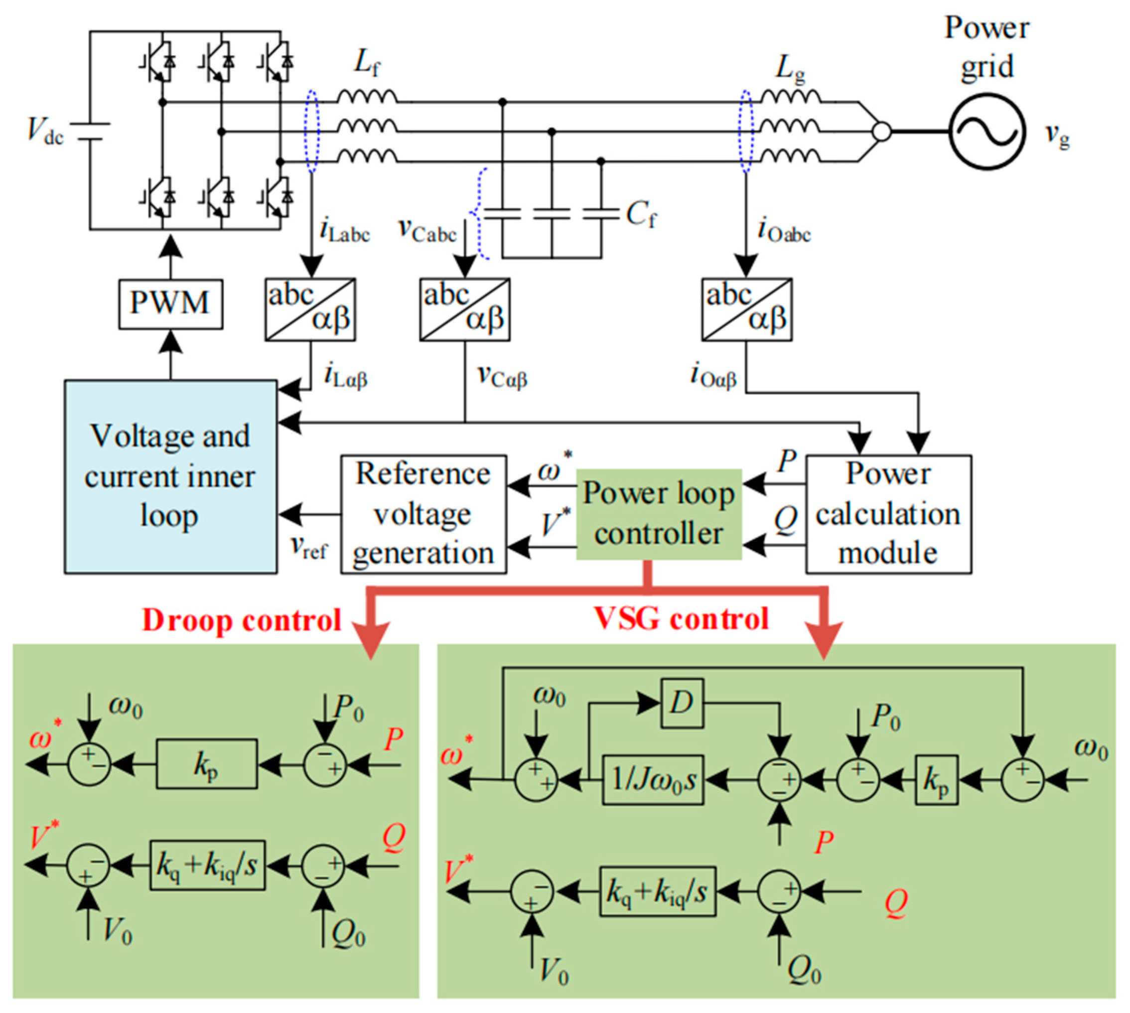
The control block diagram of the grid-forming inverter is shown in Figure 1. This paper takes the three-phase system as an example, and the main circuit is composed of a DC source (V_dc), a three-phase half-bridge inverter circuit, an LC filter, and a line inductor (L_g). The controller generally consists of a power control loop, a capacitor voltage control loop, and an inductor current control loop. The most commonly used control methods for power loops include droop control and VSG control. Figure 1 shows the principles of these two control methods at the same time. Both of them simulate the external characteristics of synchronous generators and generate corresponding voltage, frequency, and amplitude reference values according to the output power. It can be proven that, under certain conditions, droop control and VSG control are equivalent [22]. Therefore, droop control is chosen as an example for analysis and discussion in this paper. The conclusions drawn are equally applicable to VSG control or other control strategies for grid-forming inverters.

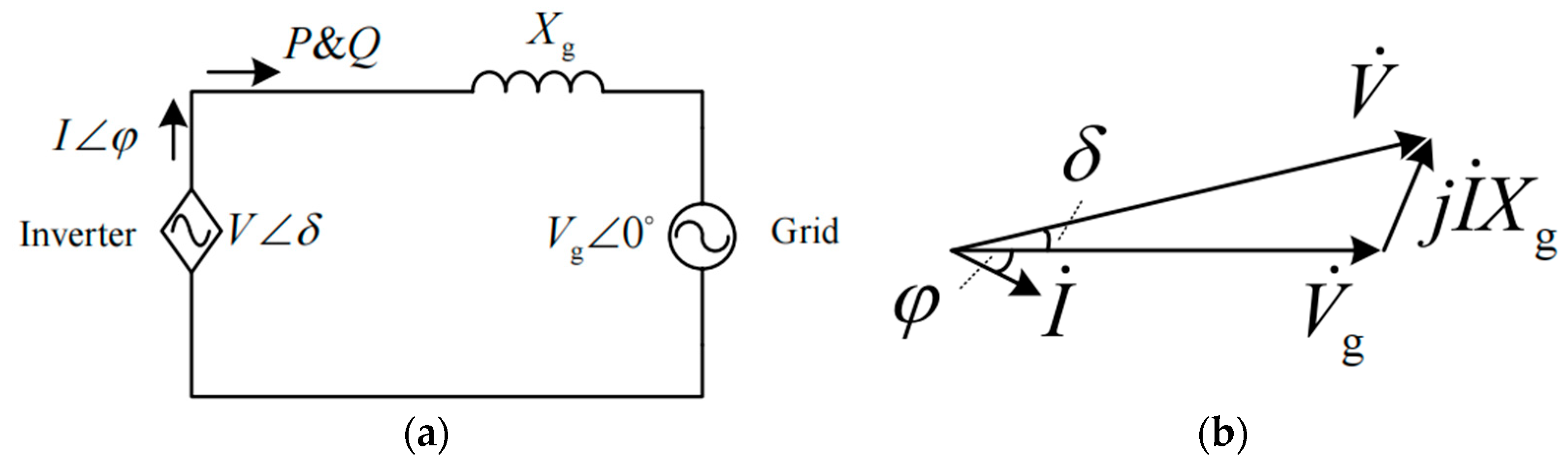
It is worth noting that the reactive power control loop is changed from a traditional proportional gain to a PI regulator to ensure that the reactive power can track the command value [23,24]. The internal voltage loop and current loop are responsible for tracking the voltage reference generated by the power loop and can improve the stability of the system. Assuming that the feeder impedance is purely inductive, the inverter output voltage can be controlled by establishing the droop characteristics of active power to phase and reactive power to voltage amplitude. Therefore, the grid-forming grid-connected inverter can be regarded as a controlled voltage source, and the system can be simplified into an equivalent circuit as shown in Figure 2a, and its corresponding phasor diagram is shown in Figure 2b.

According to the circuit principle, the inverter output active power and reactive power can be expressed as

$$\left\{\begin{array}{c}P=\frac{V_g}{X_g}V\sin \delta \hfill \\ Q=\frac{1}{X_g}\left(V^2-V_{g}V\cos \delta \right)\end{array}\right.$$

(1)

where $V\angle \delta$ is the inverter voltage, $V_g\angle 0^{\circ }$ is the power grid voltage, and $X_g$ is the line reactance.

In most literature, the analysis process for (1) is as follows: First, assuming that the phase difference δ between the inverter voltage and the grid voltage is small enough (close to zero), it can be approximated that $\sin \delta \approx \delta$ and $\cos \delta \approx 1$. On this basis, (1) can be simplified into the following form:

$$\left\{\begin{array}{c}P=\frac{V_g}{X_g}V\delta \hfill \\ Q=\frac{1}{X_g}\left(V^2-V_{g}V\right)\end{array}\right.$$

(2)

Afterward, a small signal linearization analysis is carried out on (2), and a small signal disturbance (ΔV, Δδ) is introduced to the voltage amplitude and phase difference around the steady-state operating point (V_s, δ_s), that is $V=V_s+\Delta V$, $\delta ={\delta }_s+\Delta \delta$, (2) can be expressed as:

$$\left\{\begin{array}{c}{P}_s+\Delta P=\frac{V_g}{X_g}\left(V_s+\Delta V\right)\left({\delta }_s+\Delta \delta \right)\hfill \\ Q_s+\Delta Q=\frac{1}{X_g}\left[{\left(V_s+\Delta V\right)}^2-V_g\left(V_s+\Delta V\right)\right]\end{array}\right.$$

(3)

where ΔP is the small signal component of active power and ΔQ is the small signal component of reactive power. By extracting the small signal relationship, the following model can be derived:

$$\left\{\begin{array}{c}\Delta P=\frac{V_g}{X_g}\left(V_s\Delta \delta +{\delta }_s\Delta V\right)\hfill \\ \Delta Q=\frac{2V_s-V_g}{X_g}\Delta V\hfill \end{array}\right.$$

(4)

Under the assumption that ${\delta }_s\approx 0$, the following small signal relationship can be obtained:

$$\left\{\begin{array}{c}\Delta P=\frac{V_g{V}_s}{X_g}\Delta \delta \hfill \\ \Delta Q=\frac{2V_s-V_g}{X_g}\Delta V\end{array}\right.$$

(5)

It can be seen that the active power is proportional to the phase difference and the reactive power is proportional to the voltage amplitude, and there is no power coupling issue. The widely employed droop control and VSG control leverage this conclusion by adjusting the frequency to modify the active power and adjusting the voltage amplitude to alter the reactive power.

The crucial assumption made in the above derivation is that the phase difference δ must be sufficiently small and basically constant. However, in practical systems, the phase difference does not necessarily satisfy this condition. Especially in the distributed power system, the line impedance is relatively large, and the output of the same active power requires a larger phase difference, which leads to the small signal model in (5) not being completely accurate. At this time, the accurate relationship between the inverter voltage and the grid voltage can only be accurately described through (1). Both active power and reactive power are related to the phase difference and amplitude of voltage, and there is an obvious power coupling phenomenon under this condition.

3. Proposed Power Decoupling Strategy and Modeling Analysis

To solve the power coupling issue and avoid interference between active power and reactive power control loops, a decoupling strategy based on feedforward control is proposed in this paper. The basic idea is as follows: Initially, without relying on the assumption of $\delta \approx 0$, a small-signal linearized model analysis is conducted on the power transmission model in (1). Subsequently, a frequency feedforward term is introduced into the active power control loop, and an amplitude feedforward term is introduced into the reactive power control loop. This is aimed at counteracting the inherent power coupling relationships, thereby achieving decoupled control of output power.

The small signal linearization analysis of (1) is performed near the steady-state operating point (V_s, δ_s), and the following small signal model is obtained:

$$\left[\begin{array}{c}\Delta P\\ \Delta Q\end{array}\right]=\left[\begin{array}{cc}{K}_{11}& K_{12}\\ K_{21}& K_{22}\end{array}\right]\left[\begin{array}{c}\Delta \delta \\ \Delta V\end{array}\right]$$

(6)

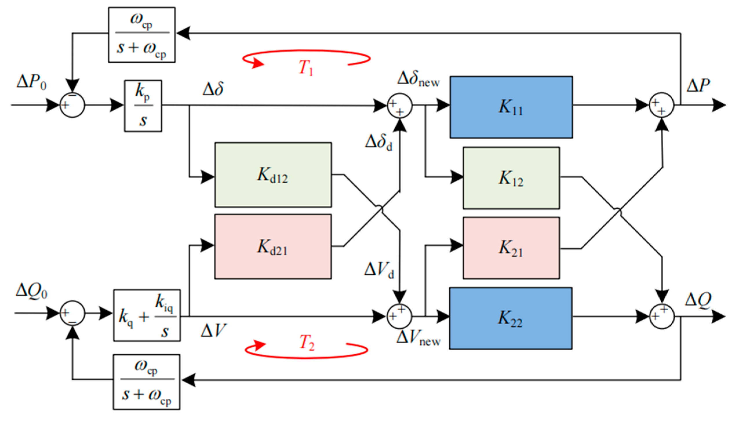
where $K_{11}=\frac{V_g{V}_s\cos {\delta }_s}{X_g}$, $K_{12}=\frac{V_g{V}_s\sin {\delta }_s}{X_g}$, $K_{21}=\frac{V_g\sin {\delta }_s}{X_g}$, $K_{22}=\frac{2V_s-V_g\cos {\delta }_s}{X_g}$. On the basis of ignoring the effect of the inner voltage and current loop, the small signal linearization model of the power loop is shown in Figure 3, which shows that there is an obvious power coupling relationship. To achieve decoupled control of power, fundamentally, it involves introducing decoupling elements into the control system to minimize the off-diagonal elements of the matrix in (6). This minimization aims to ensure that active power is primarily influenced by the phase difference and reactive power is primarily influenced by the voltage amplitude. The following sections provide separate explanations for the decoupled control principles of active power and reactive power.

The small signal linearization model of a power loop without decoupling is shown in Figure 3 above.

3.1. Active Power Decoupling Control

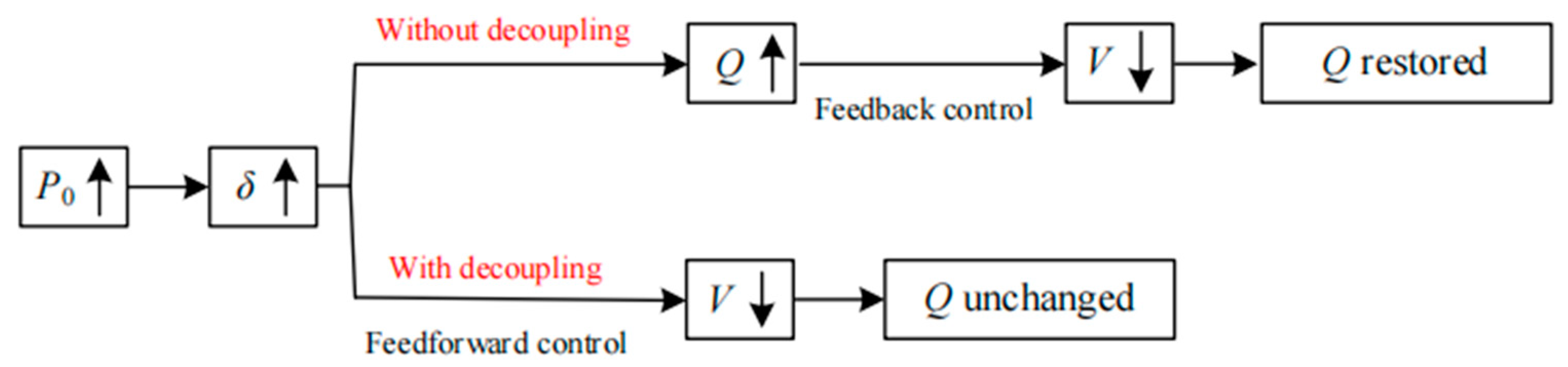
The objective of active power decoupling control is to render active power unaffected by voltage amplitude. The basic idea of active power feedforward decoupling control can be qualitatively analyzed in Figure 4. Assuming that the active power command value remains unchanged while the reactive power command value steps at a certain time, the reactive power controller will increase the voltage amplitude to track the new command value. In the absence of decoupling control, it can be seen from (1) that the increase in voltage amplitude will also lead to an increase in active power. Due to the unchanged command value for active power, the active power controller is compelled to passively decrease the phase difference through the feedback mechanism to maintain a constant output.

However, due to the lower bandwidth and slow response of the power control loop, there will inevitably be a period of active power fluctuation during this process. Conversely, if, during the voltage amplitude adjustment, the feedforward control is employed to actively reduce the phase difference, the impact of reactive power changes on active power can be counteracted, thus maintaining a constant output of active power. In this process, the active power controller is not triggered, theoretically resulting in faster response and smaller active power fluctuations, achieving decoupled control of active power. Figure 4 takes the increase in the reactive power command value as an example, and the analysis of decreasing is similar. The following derivation outlines the calculation method for the feedforward compensation of the phase difference.

According to (6), it can be deduced that:

$$\Delta P=K_{11}\Delta \delta +K_{12}\Delta V$$

(7)

Assuming that the voltage amplitude changes ΔV, to ensure the active power remains unchanged, let ΔP = 0. The phase difference required can be calculated as follows:

$$\Delta {\delta }_{\mathrm{d}}=K_{\mathrm{d}21}\Delta V=\frac{-\sin {\delta }_s}{V_s\cos {\delta }_s}\Delta V$$

(8)

where $\Delta {\delta }_{\mathrm{d}}$ is the phase difference feedforward compensation value, and K_d21 is the phase difference feedforward compensation coefficient. According to (8), the phase difference feedforward value needed to compensate for the voltage amplitude change ΔV can be calculated.

Considering that the phase difference δ_s in the actual system is generally unknown and challenging to measure, however, it can be approximately estimated through the relationship in (1), as expressed below.

$$\left\{\begin{array}{c}\sin {\delta }_s=\frac{P_s{X}_g}{V_s{V}_g}\hfill \\ \cos {\delta }_s=\frac{V_s^2-Q_s{X}_g}{V_s{V}_g}\hfill \end{array}\right.$$

(9)

According to (9), the output power can be used to calculate the phase difference. Substituting (9) into (8), another calculation method for the feedforward compensation value of the phase difference can be obtained:

$$\Delta {\delta }_{\mathrm{d}}=K_{\mathrm{d}21}\Delta V=\frac{P_s{X}_g}{Q_s{X}_g{V}_s-V_s^3}\Delta V$$

(10)

From the above analysis, (8) and (10) can both be used to calculate the phase difference feedforward value, and they are equivalent. However, considering the challenges of practical application, they each have their own advantages and disadvantages. (8) needs the voltage phase difference, and sine and cosine trigonometric operations are required. Nevertheless, line inductance information needs to be obtained in (10). Therefore, a suitable calculation method can be chosen based on the operating conditions of the practical application. Considering that the acquisition of line impedance information is generally easier than the voltage phase difference, (10) is recommended as the preferred calculation scheme.

3.2. Reactive Power Decoupling Control

The analysis process of reactive power decoupling control is similar to that of active power decoupling control, aiming to render reactive power unaffected by the voltage phase difference. The basic concept can be qualitatively analyzed, as shown in Figure 5. If the reactive power command value remains unchanged while the active power command value steps at a certain moment, the active power controller will increase the voltage phase difference to track the active power command value. Without decoupling control, according to (1), the increase in voltage phase difference will also lead to an increase in reactive power. Since the reactive power command value remains constant, the reactive power controller will passively decrease the voltage amplitude through feedback mechanisms to maintain a constant output. However, due to the low bandwidth and slow response of the power loop, there will inevitably be a period of reactive power fluctuation during this process. On the contrary, if, during the voltage phase difference adjustment, the feedforward control is employed to actively decrease the voltage amplitude, the effect of phase difference changes on reactive power can be counteracted, thus maintaining a constant output of reactive power. In this process, there is no need to trigger the reactive power controller. Theoretically, this results in faster response and smaller reactive power fluctuations, achieving decoupled control of reactive power. The following derivation outlines the calculation method for the amplitude feedforward value.

According to (6), it can be observed that:

$$\Delta Q=K_{21}\Delta \delta +K_{22}\Delta V$$

(11)

Assuming that the phase difference changes Δδ, to ensure that the reactive power in (11) remains unchanged, the required amplitude feedforward value can be calculated as follows:

$$\Delta V_{\mathrm{d}}=K_{\mathrm{d}12}\Delta \delta =\frac{V_g{V}_s\sin {\delta }_s}{V_g\cos {\delta }_s-2V_s}\Delta \delta$$

(12)

where $\Delta V_{\mathrm{d}}$ is the amplitude feedforward compensation value, and K_d21 is the amplitude feedforward compensation factor.

According to (12), the amplitude feedforward value needed to counteract the phase difference Δδ can be obtained. Similarly, to avoid measuring the voltage phase difference δ_s and the grid voltage V_g, by substituting (9) into (12), an alternative calculation method for the amplitude feedforward value can be obtained:

$$\Delta V_{\mathrm{d}}=K_{\mathrm{d}12}\Delta \delta =\frac{P_s{X}_g{V}_s}{-Q_s{X}_g-V_s^2}\Delta \delta$$

(13)

Similar to the discussion in Section 3.1, both (12) and (13) can be used to calculate the amplitude feedforward value, but with different limitations. (12) relies on the measurement of phase difference and grid voltage V_g, and sine and cosine trigonometric functions are needed. However, (13) needs to obtain the line inductance. An appropriate method can be selected according to the specific working conditions in a practical application. Since the acquisition of line impedance information is generally easier than the voltage phase difference, (13) is recommended as the preferred calculation scheme.

It is worth noting that the above derivations are based on the single-phase circuit model shown in Figure 2a. For the grid-forming grid-connected three-phase inverter system, the analysis and derivation process are basically the same, except that there are slight differences in the calculation equations of the feedforward values. The relationship between phase difference and output power shown in (9) in three-phase systems should be written as:

$$\left\{\begin{array}{c}\sin {\delta }_s=\frac{P_s{X}_g}{3V_s{V}_g}\hfill \\ \cos {\delta }_s=\frac{3V_s^2-Q_s{X}_g}{3V_s{V}_g}\hfill \end{array}\right.$$

(14)

Accordingly, the equation for calculating the phase difference feedforward value and amplitude feedforward value in a three-phase inverter should be:

$$\Delta {\delta }_{\mathrm{d}}=K_{\mathrm{d}21}\Delta V=\frac{-\sin {\delta }_s}{V_s\cos {\delta }_s}\Delta V=\frac{P_s{X}_g}{Q_s{X}_g{V}_s-3V_s^3}\Delta V$$

(15)

$$\Delta V_{\mathrm{d}}=K_{\mathrm{d}12}\Delta \delta =\frac{V_g{V}_s\sin {\delta }_s}{V_g\cos {\delta }_s-2V_s}\Delta \delta =\frac{P_s{X}_g{V}_s}{-Q_s{X}_g-3V_s^2}\Delta \delta$$

(16)

Taking into account the aforementioned phase feedforward and amplitude feedforward, the small-signal linearized model of the power loop with decoupling is depicted in Figure 6.

3.3. Application of the Decoupling Method in the Actual System

The phase and amplitude feedforward values derived in Section 3.1 and Section 3.2 are both based on the small-signal model shown in (6). According to the feedforward calculation equations given in (10) and (13), to apply this decoupling method to an actual controller, the variables that need to be monitored are the changes in voltage amplitude and phase difference (i.e., ΔV and Δδ). This can be achieved by using the derivative algorithm (for continuous systems) or the differential algorithm (for discrete systems) on the voltage amplitude and phase difference. Additionally, the phase feedforward value and amplitude feedforward value obtained (i.e., $\Delta {\delta }_{\mathrm{d}}$ and $\Delta V_{\mathrm{d}}$) are effective only for the current control cycle. In practical applications, it is necessary to perform integration (for continuous systems) or accumulation (for discrete systems) to ensure that the feedforward values remain effective throughout the entire control process.

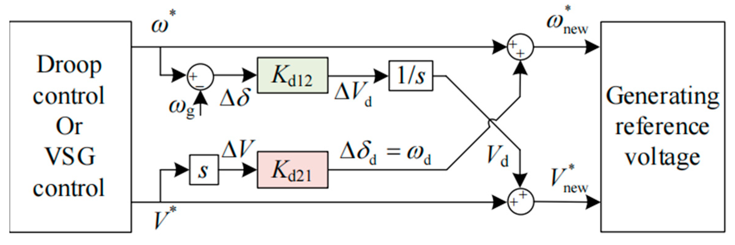
Considering the inherent integral relationship between phase and frequency, the phase difference detection in (13) can be transformed into frequency detection, eliminating the need for the differential algorithm. Similarly, the phase feedforward generated by (10) can also be converted into frequency feedforward, eliminating the need for the integral calculation. Based on the above analysis, the schematic diagram for the practical implementation of the proposed feedforward power decoupling scheme is illustrated in Figure 7.

Initially, droop control, or VSG control, generates reference values for voltage frequency and amplitude. Subsequently, by calculating the derivative of the amplitude reference value, the change in voltage amplitude is obtained. According to (10), the frequency feedforward term ω_d is calculated, which is then added to the frequency reference value generated by droop control or VSG control to obtain a new frequency reference value ω^*_new, thereby achieving active power decoupling control. Simultaneously, by computing the difference between the frequency reference value and the grid frequency, the change in phase difference is obtained. According to (13) and through integration, the voltage feedforward term V_d is determined. This term is added to the amplitude reference value generated by droop control or VSG control to produce a new amplitude reference value, V^*_new, thereby achieving reactive power decoupling control. Finally, the reference voltage for the inner voltage loop is generated by ω^*_new and V^*_new.

The application schematic diagram of the proposed feedforward power decoupling scheme is shown in Figure 7 above.

3.4. System Modeling Analysis

According to the small signal linearization model of the power control loop before and after adding the decoupling link shown in Figure 3 and Figure 6, the validity of the proposed power decoupling strategy can be verified theoretically. Considering that the bandwidth of the power loop is much lower than that of the inner voltage and current loop, the small signal model only considers the dynamic characteristics of the power loop and ignores the inner voltage and current loop.

In accordance with the power control model depicted in Figure 3 without decoupling, the open-loop transfer functions of the active power and reactive power control loops can be expressed using T₁ and T₂, respectively, as follows:

$$T_1=\frac{K_{11}{k}_{\mathrm{p}}{\omega }_{\mathrm{cp}}}{s\left(s+{\omega }_{\mathrm{cp}}\right)}$$

(17)

$$T_2=\frac{K_{22}{\omega }_{\mathrm{cp}}\left(k_{\mathrm{q}}s+k_{\mathrm{iq}}\right)}{s\left(s+{\omega }_{\mathrm{cp}}\right)}$$

(18)

On this basis, the closed-loop transfer function from the command values of active power and reactive power to the output values can be derived. Due to the coupling effect, the transfer function is in matrix form, as shown below:

$$\left[\begin{array}{c}\Delta P\\ \Delta Q\end{array}\right]=\left[\begin{array}{cc}{G}_{11}& G_{12}\\ G_{21}& G_{22}\end{array}\right]\left[\begin{array}{c}\Delta P_0\\ \Delta Q_0\end{array}\right]$$

(19)

The expressions for each element of the matrix are as follows:

$$G_{11}=\frac{K_{11}{k}_{\mathrm{p}}}{s\left(1+T_1\right)}, G_{12}=\frac{K_{21}\left(k_{\mathrm{q}}s+k_{\mathrm{iq}}\right)}{s\left(1+T_2\right)}, G_{21}=\frac{K_{12}{k}_{\mathrm{p}}}{s\left(1+T_1\right)}, G_{22}=\frac{K_{22}\left(k_{\mathrm{q}}s+k_{\mathrm{iq}}\right)}{s\left(1+T_2\right)}$$

According to Figure 6, the open-loop transfer functions of the active power and reactive power control loops are still T₁ and T₂ after the decoupling link is added. However, the expression of the closed-loop transfer function changes to the following expression due to the addition of the decoupling:

$$\left[\begin{array}{c}\Delta P\\ \Delta Q\end{array}\right]=\left[\begin{array}{cc}{G}_{\mathrm{d}11}& G_{\mathrm{d}12}\\ G_{\mathrm{d}21}& G_{\mathrm{d}22}\end{array}\right]\left[\begin{array}{c}\Delta P_0\\ \Delta Q_0\end{array}\right]$$

(20)

The expressions for each element of the matrix are as follows:

$$\begin{gathered} G_{\mathrm{d}11}=G_{11}=\frac{K_{11}{k}_{\mathrm{p}}}{s\left(1+T_1\right)}, G_{\mathrm{d}12}=\frac{K_{21}\left(k_{\mathrm{q}}s+k_{\mathrm{iq}}\right)\left(1+T_1\right)+K_{11}{K}_{\mathrm{d}21}\left(k_{\mathrm{q}}s+k_{\mathrm{iq}}\right)}{s\left(1+T_1\right)\left(1+T_2\right)}, \\ G_{\mathrm{d}21}=\frac{K_{12}{k}_{\mathrm{p}}\left(1+T_2\right)+K_{22}{K}_{\mathrm{d}12}{k}_{\mathrm{p}}}{s\left(1+T_1\right)\left(1+T_2\right)}, G_{\mathrm{d}22}=G_{22}=\frac{K_{22}\left(k_{\mathrm{q}}s+k_{\mathrm{iq}}\right)}{s\left(1+T_2\right)} \end{gathered}$$

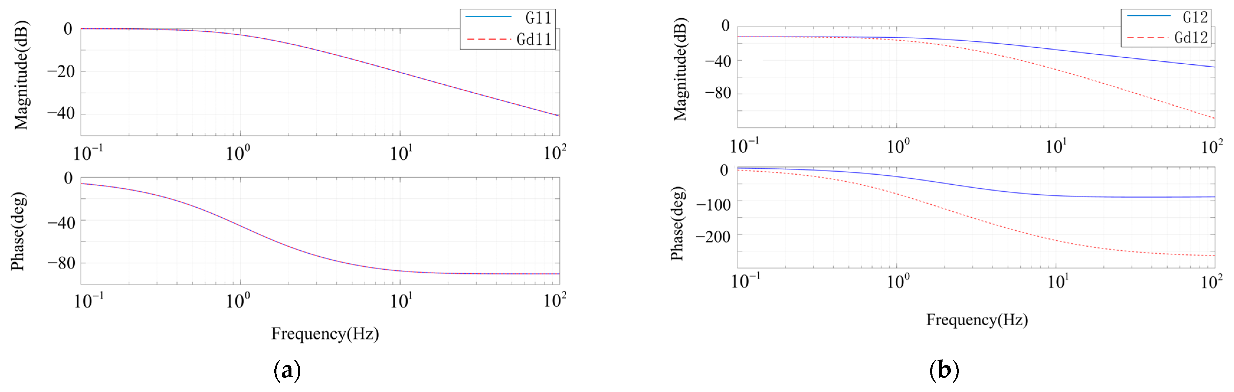
According to the closed-loop transfer functions in (19) and (20), the bode diagram of the closed-loop transfer function of the system is shown in Figure 8. It can be seen from the bode diagram that the addition of the decoupling network has basically no effect on the diagonal elements, but the magnitude of the off-diagonal elements decreases significantly after the addition of the decoupling network, which proves that the decoupling scheme can significantly suppress the coupling of active power and reactive power control loops.

The bode diagram of the closed-loop transfer function is shown in Figure 8 above.

4. Simulation and Hardware Verification

To verify the effectiveness of the power decoupling strategy proposed in this paper, simulation in the PSCAD/EMTDC environment and hardware verification on a 9 kVA prototype have been carried out. The topology of the system in simulation and experiment is the same as that in Figure 1. The power loop adopts droop control. The power stage and controller parameters are shown in

Table 1. Simulation and hardware parameters of grid-forming grid-connected inverter.

Symbol and Meaning	Simulation Parameter	Hardware Parameter
DC voltage Vdc/V	600	600
Capacity of the inverter S/kVA	/	9
Switching frequency fs/kHz	10	12.5
Filter inductance Lf/mH	2.7	3
Filter capacitance Cf/μF	15	30
Line inductance Lg/mH	5	8
The cut-off frequency of the low-pass filter in the power calculation module ωcp/(rad/s)	62	31
P-ω Droop coefficient kp/(rad/s/W)	6.28 × 10−4	6.28 × 10−4
Q-V Droop coefficient kq/(V/var)	4 × 10−6	6 × 10−6
Q-V Integral coefficient kiq	0.1	0.2
Rated frequency ω0/(rad/s)	100 π	100 π
RMS value of rated phase voltage V0/V	115	115

. The fundamental idea of verification involves changing the command value of either active power or reactive power while keeping the command value of the other power channel constant. By comparing the magnitude of fluctuations in the output active power and reactive power before and after the introduction of the decoupling network, the effectiveness of the proposed scheme can be verified.

The simulation and hardware parameters are as shown in Table 1 above.

4.1. Simulation Verification

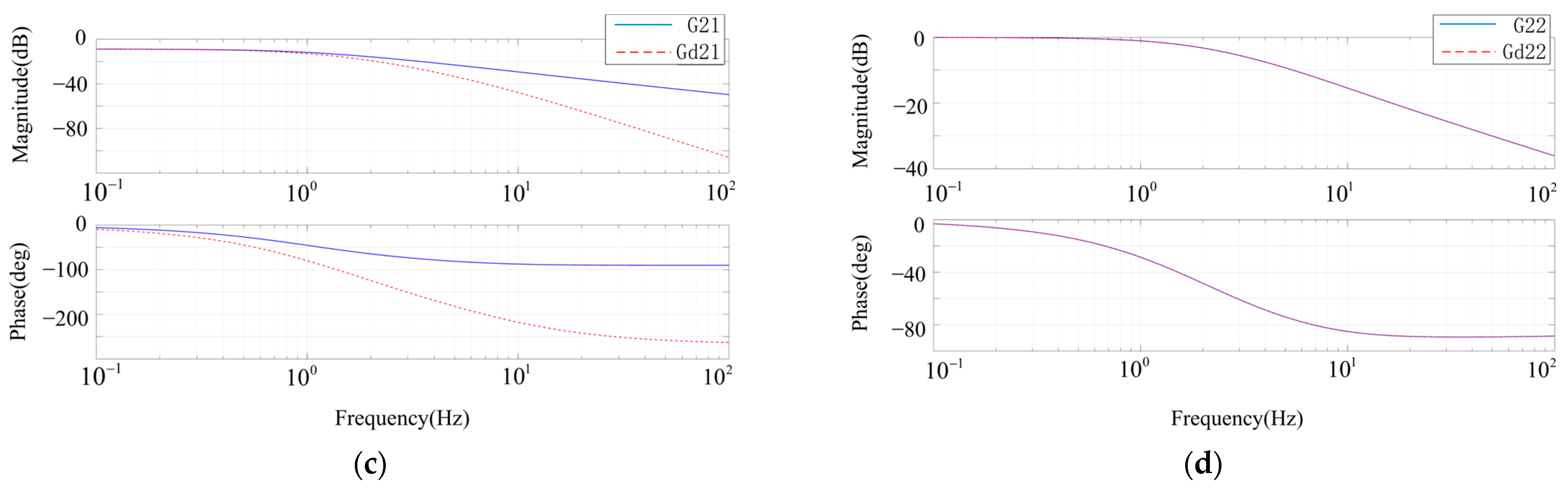
At the beginning of the simulation, the active power command value is 10 kW, and the reactive power command value is 0 kvar. When t = 2.0 s, the active power command changes from 10 kW to 5 kW and then changes back to 10 kW at t = 3.0 s. The reactive power command value remains unchanged at 0 kvar to verify the decoupling effect of reactive power. The waveforms of output active power and reactive power in this process are shown in Figure 9a. When the decoupling is not added, the reactive power fluctuates significantly, and the recovery takes a long period of time with the change in the active power command value. By adding the amplitude feedforward decoupling, the reactive power fluctuation is greatly reduced during the change of the active power command value, which proves the effectiveness of reactive power decoupling control. Furthermore, the active power waveforms before and after the introduction of the decoupling network essentially overlap, confirming that amplitude feedforward decoupling has minimal impact on active power.

Similarly, the reactive power command value increases from 0 kvar to 6 kvar at t = 4.0 s and restores to 0 kvar at 5.0 s. While the active power command value remains unchanged at 10 kW to verify the decoupling control effect of active power. The waveform of the inverter output power in this process is shown in Figure 9b. The active power fluctuates significantly and recovers over a long period of time without the decoupling network. By adding the proposed frequency-feedforward decoupling scheme, the fluctuation of active power is greatly reduced, which proves the effectiveness of the active power decoupling control. In addition, the reactive power waveform before and after adding the decoupling network basically overlaps, which proves that the frequency feedforward decoupling has no effect on the reactive power.

4.2. Hardware Verification

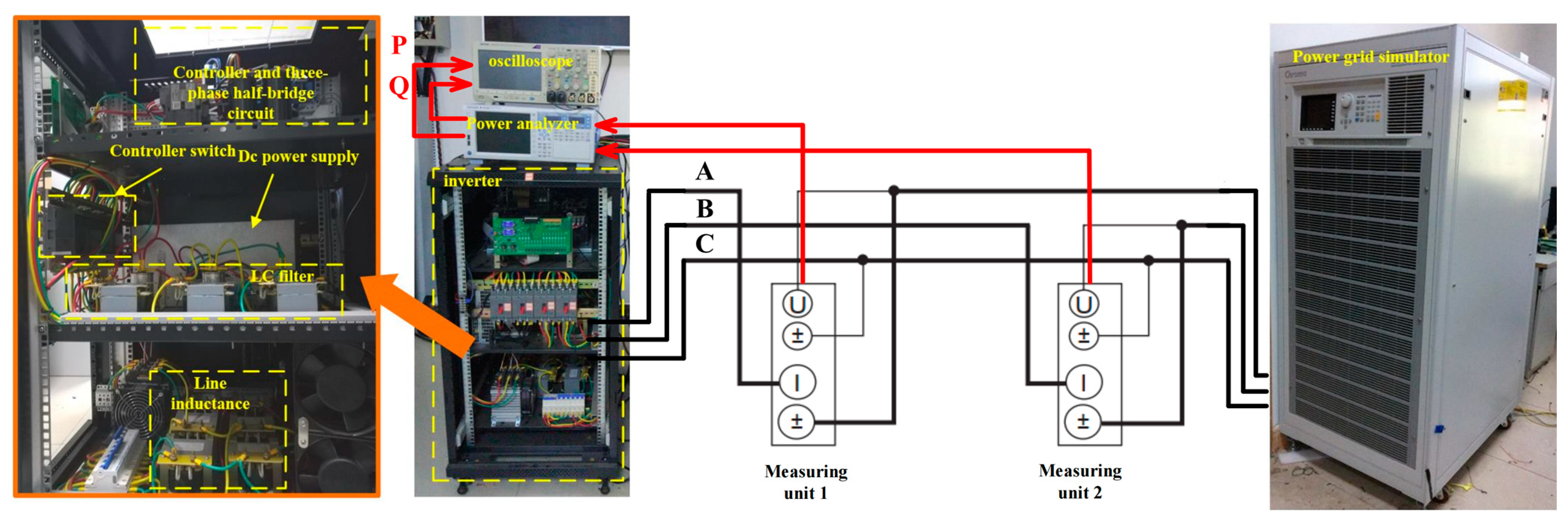
The hardware platform, as shown in Figure 10, consists of a three-phase inverter and a power grid simulator. The grid-forming grid-connected inverter has a capacity of 9 kVA and is mainly composed of a DC power supply, a three-phase inverter, an LC filter, and line impedance. The power stage and control parameters are shown in Table 1. The controller of the inverter adopts a DSP from Texas Instruments (TMS320F28335). The inverter output power is measured using a power analyzer (YOKOGAWA WT1804E). The Two-Wattmeter Method is employed to separately measure the active and reactive power output of the inverter, and the specific measurement principles and connections are illustrated in Figure 10. The power analyzer has been calibrated as required before the measurement. Since the power analyzer lacks waveform display capability, the measured power data are output through the digital-to-analog converter (DAC) channel of the power analyzer and displayed on an oscilloscope. A power grid simulator (Chroma 61860) is used to simulate the power grid.

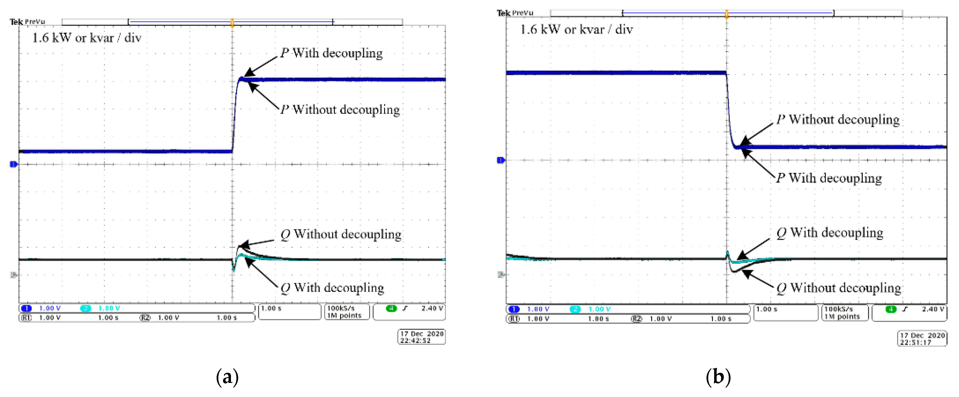
The hardware experimental process is similar to the simulation. In Figure 11a, the active power command value steps from 0.8 kW to 5 kW, and in Figure 11b, the active power command value steps from 5 kW to 0.8 kW. In the whole process, the reactive power remains unchanged at 0.8 kvar. It can be seen that without decoupling, the reactive power fluctuates significantly with the change in the active power command value. After adding the amplitude feedforward decoupling control, the fluctuation of the reactive power is significantly reduced, and the recovery speed is greatly improved, which proves the effectiveness of the reactive power decoupling control. In addition, the active power waveform before and after introducing the decoupling control is basically overlapping, which proves that the amplitude feedforward decoupling control has no effect on the active power.

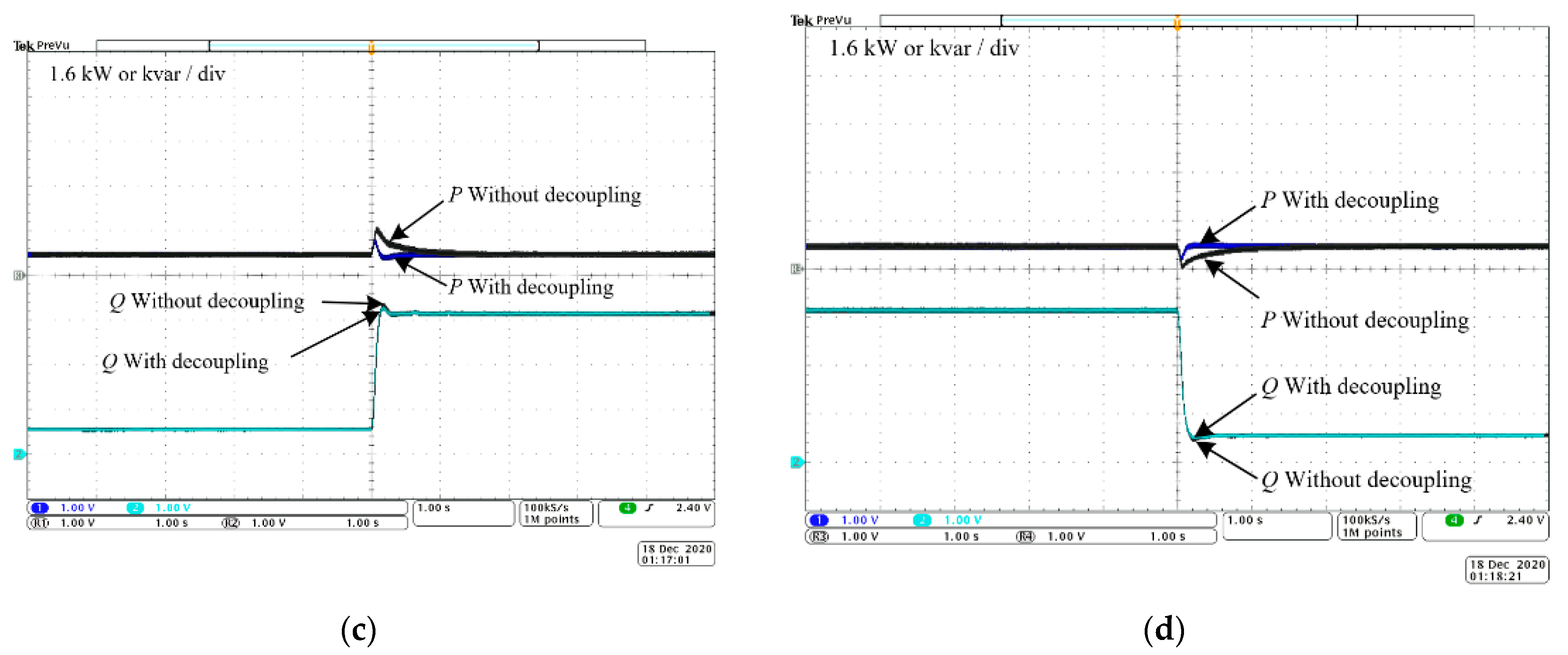
The process of reactive power command value change is shown in Figure 11c,d. In Figure 11c, the reactive power command value steps from 0.8 kvar to 5 kvar, and in Figure 11d, the reactive power command value steps from 5 kvar to 0.8 kvar. The active power command value remained unchanged at 0.8 kW throughout the process. It can be seen that the active power fluctuates significantly with the change in the reactive power command value when there is no decoupling. After the frequency feedforward decoupling control is added, the fluctuation of the active power is significantly reduced, and the recovery speed is greatly improved, which proves the effectiveness of the active power decoupling control. In addition, the reactive power waveform before and after introducing the decoupling control is basically overlapping, which proves that the frequency feedforward decoupling control has no effect on the reactive power.

Through the above simulation and hardware experimental results, it can be proven that the proposed power decoupling strategy can effectively suppress the coupling between active power and reactive power without affecting the tracking characteristics of the power controller. It has a significant effect on realizing power-independent control and improving system performance. The limitation of this method is that, due to the feedforward control method, there is a certain compensation error in practice, and small fluctuations can be seen in the simulation and experiment.

5. Conclusions

When the grid-forming inverter works in parallel with a microgrid or large grid, the output active power and reactive power will be coupled due to the large voltage phase difference. Aiming at this power coupling problem, a decoupling strategy based on frequency feedforward and amplitude feedforward is proposed to realize the decoupling control of active power and reactive power, respectively. The proposed decoupling strategy exhibits two key advantages: firstly, it directly modifies the voltage reference values through feedforward, offering a straightforward and easily implementable principle; secondly, it is applicable to various control coordinate systems (such as dq coordinate systems, αβ coordinate systems, etc.) and control structures without inner current loops, ensuring a broad range of applicability. Finally, the effectiveness of the power decoupling strategy is further verified by simulation and experiment.

The inverter decoupling method we propose holds promising application prospects and potential commercial value. Here are the potential application areas and related commercial values of this method: The application of this decoupling method in renewable energy systems, such as solar and wind energy conversion, is expected to enhance energy conversion efficiency and reduce energy losses in the system. Applying the inverter decoupling method to power electronics equipment has the potential to improve performance, reduce harmonics, and enhance system stability, thereby driving further developments in power electronics equipment. The inverter decoupling method holds crucial significance for microgrid and island operation systems. By improving the control precision of inverters, more reliable and efficient microgrid operation can be achieved, providing sustainable power support for island operations.

Since the essay focuses on the decoupling control of one inverter, our future work will focus on power decoupling control for grid-forming inverters in islanded mode and multi-inverter parallel systems.

References

- Hu, J.; Shan, Y.; Cheng, K.W.; Islam, S. Overview of Power Converter Control in Microgrids—Challenges, Advances, and Future Trends. IEEE Trans. Power Electron. 2022, 37, 9907–9922. [Google Scholar] [CrossRef]
- Wang, J.; Ma, K. Inertia and Grid Impedance Emulation of Power Grid for Stability Test of Grid-Forming Converter. IEEE Trans. Power Electron. 2023, 38, 2469–2480. [Google Scholar] [CrossRef]
- Awal, M.A.; Yu, H.; Husain, I.; Yu, W.; Lukic, S.M. Selective Harmonic Current Rejection for Virtual Oscillator Controlled Grid-Forming Voltage Source Converters. IEEE Trans. Power Electron. 2020, 35, 8805–8818. [Google Scholar] [CrossRef]
- Awal, M.A.; Rachi, M.R.K.; Yu, H.; Husain, I.; Lukic, S. Double Synchronous Unified Virtual Oscillator Control for Asymmetrical Fault Ride-Through in Grid-Forming Voltage Source Converters. IEEE Trans. Power Electron. 2023, 38, 6759–6763. [Google Scholar] [CrossRef]
- Ziwen, L.I.; Shihong, M.I.O.; Zhihua, F.A. Accurate power allocation and zero steady-state error voltage control of the islanding DC microgrid based on adaptive droop characteristics. Trans. China Electrotech. Soc. 2019, 34, 795–806. [Google Scholar]
- Jieyi, X.U.; Wei, L.I.; Shu, L.I.; Fujie, C.H.N.; Xiaorong, X.I. Current State and Development Trends of Power System Converter Grid-forming Control Technology. Power Syst. Technol. 2022, 46, 3586–3594. [Google Scholar]
- Hu, Q. Grid-Forming Inverter Enabled Virtual Power Plants with Inertia Support Capability. IEEE Trans. Smart Grid. 2022, 13, 4134–4143. [Google Scholar] [CrossRef]
- Eid, B.M.; Rahim, N.A.; Selvaraj, J. Control Methods and Objectives for Electronically Coupled Distributed Energy Resources in Microgrids: A Review. IEEE Syst. J. 2016, 10, 446–458. [Google Scholar] [CrossRef]
- Guerrero, J.M.; de Vicuna, L.G.; Matas, J.; Castilla, M.; Miret, J. Output impedance design of parallel-connected UPS inverters with wireless load-sharing control. IEEE Trans. Ind. Electron. 2005, 52, 1126–1135. [Google Scholar] [CrossRef]
- Rodríguez-Cabero, A.; Roldán-Pérez, J.; Prodanovic, M. Virtual Impedance Design Considerations for Virtual Synchronous Machines in Weak Grids. IEEE J. Emerg. Sel. Topics Power Electron. 2020, 8, 1477–1489. [Google Scholar] [CrossRef]
- Hou, G.; Xing, F.; Yang, Y.; Zhang, J. Virtual negative impedance droop method for parallel inverters in microgrids. In Proceedings of the 2015 IEEE 10th Conference on Industrial Electronics and Applications (ICIEA), Auckland, New Zealand, 15–17 June 2015; pp. 1009–1013. [Google Scholar]
- Guerrero, J.M.; Matas, J.; de Vicuna, L.G.; Castilla, M.; Miret, J. Decentralized Control for Parallel Operation of Distributed Generation Inverters Using Resistive Output Impedance. IEEE Trans. Ind. Electron. 2007, 54, 994–1004. [Google Scholar] [CrossRef]
- Zhang, H.; Kim, S.; Sun, Q.; Zhou, J. Notice of Removal: Distributed Adaptive Virtual Impedance Control for Accurate Reactive Power Sharing Based on Consensus Control in Microgrids. IEEE Trans. Smart Grid. 2017, 8, 1749–1761. [Google Scholar] [CrossRef]
- Wang, X.; Li, Y.W.; Blaabjerg, F.; Loh, P.C. Virtual-Impedance-Based Control for Voltage-Source and Current-Source Converters. IEEE Trans. Power Electron. 2015, 30, 7019–7037. [Google Scholar] [CrossRef]
- He, J.; Li, Y.W. Analysis, Design, and Implementation of Virtual Impedance for Power Electronics Interfaced Distributed Generation. IEEE Trans. Ind. Appl. 2011, 47, 2525–2538. [Google Scholar] [CrossRef]
- Ren, M.; Li, T.; Shi, K.; Xu, P.; Sun, Y. Coordinated Control Strategy of Virtual Synchronous Generator Based on Adaptive Moment of Inertia and Virtual Impedance. IEEE J. Emerg. Sel. Topic Circuits Syst. 2021, 11, 99–110. [Google Scholar] [CrossRef]
- Banerjee, D.; Saxena, A.; Hashmi, M.S. A Novel Concept of Virtual Impedance for High Frequency Tri-Band Impedance Matching Networks. IEEE Trans. Circuits Syst. II Exp. Briefs 2018, 65, 1184–1188. [Google Scholar] [CrossRef]
- Liang, X.; Andalib-Bin-Karim, C.; Li, W.; Mitolo, M.; Shabbir, M.N.S.K. Adaptive Virtual Impedance-Based Reactive Power Sharing in Virtual Synchronous Generator Controlled Microgrids. IEEE Trans. Ind. Appl. 2021, 57, 46–60. [Google Scholar] [CrossRef]
- De Brabandere, K.; Bolsens, B.; Van den Keybus, J.; Woyte, A.; Driesen, J.; Belmans, R. A Voltage and Frequency Droop Control Method for Parallel Inverters. IEEE Trans. Power Electron. 2007, 22, 1107–1115. [Google Scholar] [CrossRef]
- Wu, T.; Liu, Z.; Liu, J.; Wang, S.; You, Z. A Unified Virtual Power Decoupling Method for Droop-Controlled Parallel Inverters in Microgrids. IEEE Trans. Power Electron. 2016, 31, 5587–5603. [Google Scholar] [CrossRef]
- Li, Y.; Li, Y.W. Power Management of Inverter Interfaced Autonomous Microgrid Based on Virtual Frequency-Voltage Frame. IEEE Trans. Smart Grid. 2011, 2, 30–40. [Google Scholar] [CrossRef]
- Meng, X.; Liu, J.; Liu, Z. A Generalized Droop Control for Grid-Supporting Inverter Based on Comparison between Traditional Droop Control and Virtual Synchronous Generator Control. IEEE Trans. Power Electron. 2019, 34, 5416–5438. [Google Scholar] [CrossRef]
- Deng, Y.; Tao, Y.; Chen, G. Enhanced Power Flow Control for Grid-Connected Droop-Controlled Inverters with Improved Stability. IEEE Trans. Ind. Electron. 2017, 64, 5919–5929. [Google Scholar] [CrossRef]
- Li, Y.W.; Vilathgamuwa, D.M.; Loh, P.C. Design, analysis, and real-time testing of a controller for multibus microgrid system. IEEE Trans. Power Electron. 2004, 19, 1195–1204. [Google Scholar] [CrossRef]