Load Day-Ahead Automatic Generation Control Reserve Capacity Demand Prediction Based on the Attention-BiLSTM Network Model Optimized by Improved Whale Algorithm

Abstract

Load forecasting is a research hotspot in academia; in the context of new power systems, the prediction and determination of load reserve capacity is also important. In order to adapt to new forms of power systems, a day-ahead automatic generation control (AGC) reserve capacity demand prediction method based on the Fourier transform and the attention mechanism combined with a bidirectional long and short-term memory neural network model (Attention-BiLSTM) optimized by an improved whale optimization algorithm (IWOA) is proposed. Firstly, based on the response time, Fourier transform is used to refine the distinction between various types of load reserve demand, and the power of the AGC reserve band is calculated using Parseval’s theorem to obtain the reserve capacity demand sequence. The maximum mutual information coefficient method is used to explore the relevant influencing factors of the AGC reserve sequence concerning the data characteristics of the AGC reserve sequence. Then, the historical daily AGC reserve demand sequences with relevant features are input into the Attention-BiLSTM prediction model, and the improved whale algorithm is used to automatically find the optimal hyperparameters to obtain better prediction results. Finally, the arithmetic simulation results show that the model proposed in this paper has the best prediction performance with the upper (0.8810) and lower (0.6651) bounds of the coefficient of determination ($R^2$) higher than the other models, and it has the smallest mean absolute percentage error ($MAPE$) and root mean square error ($RMSE$).

1. Introduction

Automatic generation control (AGC) is the automatic adjustment of power imbalance from seconds to minutes [1,2]. The factors leading to power imbalance are load fluctuations and fluctuations in the output of new energy sources such as wind power and photovoltaic. Unplanned fluctuations in renewable energy sources and loads pose challenges to the security and stability of the power system and the balance between energy supply and demand [3,4]. Inertia is an integral and important part of future power systems [5], yet the new energy itself has a small moment of inertia [6,7,8,9], which is also unfavorable for the power system. New energy output is characterized by high volatility and randomness; while the penetration of new energy sources in the power system is increasing, the power system needs to prepare more reserve capacity to cope with the volatility of their output [10,11]. But due to the crowding out of the feed-in space of conventional thermal power units [12], the hot reserve resources available for systems are further reduced, thus posing a great challenge to the security and stability of the power system [13,14,15]. In the electricity market, ancillary services provide additional support for source–load power mismatch [16,17]. AGC is not only an important technical means to ensure the active balance of the power system and maintain frequency stability at all times [18] but also an important part of auxiliary services [19]. The dispatch and operation departments as well as the power market operators need to carry out a scientific and effective quantitative assessment of the AGC reserve demand [20]. This enables a better allocation of limited system reserve resources and ensures an efficient response to load fluctuations, thereby guaranteeing the safe and stable operation of the power system.

The current methods for determining AGC reserve capacity can be categorized into three types, which are the dispatcher’s empirical method, the probabilistic statistical method and the data-driven method, they are briefly described as follows:

(1)

The dispatcher’s experiential method refers to the approach where the system operator, based on their extensive operational experience, directly determines the AGC reserve requirements of the system by considering the electric load levels and the periodic patterns of load consumption. Alternatively, based on their operational experience, the dispatcher may calculate the AGC reserve requirements using pre-defined computational formulas and actual operational data [21]. Although this method is simple and fast, it still has the disadvantage of being insufficiently objective to be generalized on a large scale, and it is not well adapted to new power systems.

(2)

Research paper [22,23] models the load forecast error with a probability density function and calculates the AGC reserve capacity demand under a certain confidence space. Paper [24] proposes a method to control the AGC reserve capacity in the region based on the evaluation criteria correction background. Paper [25] first separates the load components and then uses statistical and other methods to determine the demand for AGC reserve capacity. However, this mathematical description is inadequate whether a normal distribution function or a t-distribution function is used.

(3)

The data-driven approach utilizes the characteristics of big data in the power system and employs a neural network model to predict the regulation capability of the AGC. Paper [26] calculates the initial capacity of the AGC from line, load, new energy and unit perspectives and predicts the capacity of the AGC using long short-term memory neural networks (LSTM). However, it still has the disadvantages that the calculation time scales are too coarse. So, it is unable to conduct a fine analysis of reserve demand, and the adaptability with the new type of power system is not good.

The characteristics of the above methods are shown in

Table 1. Characteristics of the AGC reserve capacity determination method.

Methodology	Source	Vantage	Drawback
Dispatcher’s empirical method	[21]	Simple and fast	Not well adapted to new power systems
Probabilistic statistical method	[22,23,24,25]	Comprehensive and accurate calculations	Insufficient mathematical description
Data-driven method	[26]	Based on big data and higher credibility	Time scales are too loose

. It should be noted that it takes time for the capacity reserve service to be put in place. If the reserve capacity cannot be put in place in time, it may lead to a directional loss of system control or grid collapse. Therefore, the size of the reserve capacity and the response time must be carefully considered and designed to ensure the reliability and stability of the power system. The calculation and management of the AGC reserve capacity of the above methods do not take into account the physical characteristics of the system reserve resources nor do they provide a more fine-grained division of the system reserve in terms of response time. Thus, they have limited significance in guiding the trading of reserve services under the spot market.

In recent years, the field of prediction has witnessed significant advancements due to the rapid development and widespread use of deep learning techniques. With the advent of big data, the combination of data-driven and model-driven research methods has proven to be highly effective in prediction tasks [27,28,29,30]. One notable data-driven method is the bidirectional long short-term memory (BiLSTM), which represents an improvement over the traditional LSTM by incorporating sequence information from both past and future directions. This enhanced capability of extracting time-series information has led to the widespread adoption of BiLSTM in various domains: a method for joint load forecasting in multi-energy systems based on bidirectional long short-term memory (BiLSTM) and multi-task learning is proposed in paper [31]. The emphasis of the method is on fully utilizing the coupling relationships among multiple loads; its effectiveness and superiority in terms of learning speed and prediction accuracy have been validated through case studies. Paper [32] introduced a novel stock price prediction model utilizing a bidirectional LSTM network for training and predicting stock datasets. The results of this study showcased the high application value of the proposed model. Paper [33] uses a BiLSTM network to classify peer reviews in terms of cognitive content and affective states; the results show that the BiLSTM network model achieves good results in terms of classification performance and consistency with manual coding. Paper [34] employed a prediction model based on gray relational analysis and bidirectional long short-term memory neural networks (BiLSTMs) to forecast the air quality index of several cities. The results demonstrated the model’s high prediction accuracy and its applicability across different locations.

When using neural networks for prediction, it is not simply a matter of inputting feature and label data into the model and training it directly, but it is also necessary to adjust the hyperparameters that come with the model in order to change the structure of the model so that the model achieves the best performance under different tasks. The improved whale algorithm (IWOA) is widely used as a heuristic algorithm in hyperparameter optimization. Paper [35] introduces the improved whale optimization algorithm (IWOA), which continuously optimizes the nonlinear weights of the Elman neural network during the iterative process. Paper [36,37] uses an improved whale algorithm to optimize the hidden layer of the LSTM network, the number of neurons in the first LSTM layer, etc. Paper [38] obtained a proposed IWOA optimization algorithm by improving the whale optimization algorithm (WOA). Using this algorithm to optimize the hyperparameters of the TCN-Attention model, the optimal prediction is finally obtained. In paper [39], IWOA optimizes the initial weights and thresholds of the back-propagation (BP) neural network, which speeds up the iteration speed of the BP neural network and enhances the optimization ability and robustness of the model. In paper [40], IWOA is used to find the optimal parameter values of pulse coupled neural network (PCNN) to optimize PCNN. By combining the aforementioned components, the IWOA-PCNN model had the best image denoising performance, and the produced images were crisper and preserve more information. Paper [41], in order to improve the classification effect of PNN, designed an IWOA based on the opposite-based learning (OBL) strategy and the crisscross optimization algorithm to select the optimal smoothing factor, namely IWOA-PNN. In paper [42], a transformer oil kinematic viscosity detection model based on the IWOA optimized radial basis function (RBF) neural network and multi-frequency ultrasonic detection technology is proposed; then, the IWOA-RBF training experiment samples are used to obtain the transformer oil kinematic viscosity detection model. Experimental results prove that the detection model has certain practicability.

The rapid development and increasing maturity of deep learning have opened up diverse possibilities for applications in the field of prediction. In this study, based on paper [26], a data-driven approach is employed. We leverage the excellent performance of deep learning in forecasting and combine it with the big data background of the power system to address the issue that current AGC reserve capacity determination methods do not consider the input time of reserve services. We propose considering the response time of the AGC reserve as the starting point for decomposing the net load fluctuation within a day. Furthermore, we determine the AGC reserve capacity demand for specific time periods based on the time–frequency relationship obtained through Fourier transform [43]. This approach allows for a fine-grained analysis and management of reserve capacity throughout the day. To forecast the load AGC reserve capacity demand, we employ the IWOA-Attention-BiLSTM model to fully exploit the mapping relationship between the time series characteristics of the historical day and the AGC reserve capacity demand on the day to be forecasted. By leveraging this model, we can accurately predict the load AGC reserve capacity demand. These prediction results, with a certain level of accuracy assurance, hold significant value in guiding the assessment of AGC reserve capacity demand within the reserve auxiliary service market. Overall, this study demonstrates the potential of deep learning in the field of prediction, particularly in addressing the challenges related to AGC reserve capacity determination in the power system. By integrating the IWOA-Attention-BiLSTM model and considering the time–frequency relationship, we can achieve more accurate and informed decision-making in managing AGC reserve capacity demand within the reserve auxiliary service market. The study contributes to the field in the following ways:

• This paper combines the discrete Fourier transform and Parseval’s theorem, and a method to analyze the load AGC reserve capacity requirement in fine time division is proposed.
• The method of maximizing the information coefficient is used to explore the influencing factors of AGC reserve capacity demand sequences such as meteorology and load’s change factors, and the factors with large correlation coefficients are used as the input features of the neural network prediction model.
• A prediction model for day-ahead AGC reserve capacity demand is constructed using the IWOA-Attention-BiLSTM neural network. BiLSTM is used to extract the time-series information, the attention mechanism is used to focus on the key feature factors and the improved whale optimization algorithm (IWOA) is used to optimize the hyperparameters to obtain better prediction results.

The rest of the paper is organized as follows: Section 2 introduces a refined method for analyzing load AGC reserve capacity demand. In Section 3, factors influencing the sequence of load AGC reserve capacity requirements are explored. In Section 4, the IWOA-Attention-BiLSTM prediction model is constructed. Section 5 presents a case study based on actual load sampling data from a province in southern China. Based on the analyses in Section 5, conclusions are drawn in Section 6.

2. Load AGC Reserve Capacity Determination Method

2.1. Frequency Domain Analysis Method

The discrete Fourier transform can transform a function or discrete signal in the time–frequency domain, using methods such as separation, filtering or truncation to achieve the goal of signal decomposition [44,45,46]. If $x\left(n\right)$ is a finite-length time-domain load sequence of length N, performing a DFT on it yields the corresponding finite-length frequency-domain sequence $X\left(k\right)$, which is expressed as:

$${\displaystyle X\left(k\right)=\sum _{n=0}^{N-1}x\left(n\right)·e^{-j\frac{2\pi }{N}kn},0\le n\le N-1}$$

(1)

In the above Equation (1), both n and k are integers and they are the ordinal numbers of the sampled values in the sequences $x\left(n\right)$ and $X\left(k\right)$. The relationship between n and frequency f is given by:

$$f=\frac{n{f}_s}{N}=\frac{n}{N{T}_s}$$

(2)

In the above Equation (2), $f_s$ is the sampling frequency and $T_s$ is the sampling period. The discrete Fourier transform can be viewed as the multiplication and summation of the original signal with sine and cosine signals of different frequencies. Therefore, the sinusoidal components contained in the original signal can be separated by the Fourier transform. According to the paper [47], the response time of the reserve should be the first quarter of its period, then the load frequency corresponding to the reserve should also be the reciprocal of four times the response time. The AGC response time is the time difference between the moment when the AGC command begins to change and the moment when the unit’s actual output begins to change and the change exceeds the regulation dead zone and is no longer reversed. Considering the effects of primary frequency control and thermal unit pressure pullback and allowing a certain AGC reserve capacity margin, the range of the actual AGC reserve response time of the system is determined to be (30 s, 3 min] and the load frequency corresponding to this time range is (1/720 Hz, 1/120 Hz].

The inverse discrete Fourier transform (IDFT) is the inverse of the DFT. The inverse discrete Fourier transform of a finite length sequence in the frequency domain is defined as:

$${\displaystyle x\left(n\right)=\frac{1}{N}\sum _{k=0}^{N-1}X\left(k\right)·e^{j\frac{2\pi }{N}},0\le k\le N-1}$$

(3)

Utilizing the inverse discrete Fourier transform (IDFT), the frequency domain signal can be converted into the time domain signal after classification filtering. The net load signal for a day is divided based on the frequency band to which the AGC reserve belongs. Each frequency band’s frequency domain signals are then transformed into their respective time domain signals. The decomposition results are shown in Figure 1 below.

In Figure 1, the frequency range to which the category 1 component of the load belongs is $(1/120\mathrm{Hz},\infty )$, the category 1 component of the load is characterized by a small change amplitude and short change period, so it is responded by the primary frequency regulation. The category 2 component of the load is the one corresponding to the AGC reserve. The third type of load component belongs to the frequency band of $(0, 1/720\mathrm{Hz}]$, with the characteristics of large change amplitude and long change period, and it can be used as the scheduled load curve.

2.2. AGC Reserve Capacity Calculation Method

Parseval’s theorem is widely used in the derivation of time–frequency analysis of signals [48]. It states that the energy (or power) of a signal remains equal in both the time and frequency domains. The theorem’s mathematical essence lies in the invariance of orthogonal transformations applied to signals in vector space. For a signal within the frequency range $[f_1,f_2]$, its energy can be calculated using the following Equation (4):

$$E(f_1,f_2)=\sum _{f_1}^{f_2}{\left|X\left(f\right)\right|}^2$$

(4)

In the above Equation (4), $X\left(f\right)$ denotes each spectral component, and the modulus represents the amplitude of the spectral component at the actual frequency of f. From this, the power values $P(f_1,f_2)$ in different frequency ranges can be obtained as shown in the following Equation (5):

$$P(f_1,f_2)=\sqrt{\sum _{f_1}^{f_2}{\left|X\left(f\right)\right|}^2}$$

(5)

To determine the AGC reserve capacity, the frequency range $(1/720\mathrm{Hz}, 1/120\mathrm{Hz})$ should be considered. The load curve, sampled at a 30 s interval and consisting of a total of 2880 data points for the entire day, undergoes a Fourier transform every 15 min. By applying Parseval’s theorem, the data points within the frequency range $(1/720\mathrm{Hz}, 1/120\mathrm{Hz})$ are converted to power in the time domain. The AGC reserve capacity requirement for the entire day is obtained by concatenating the results of 96 segments, each representing a 15-min interval, and the full-day demand curve is shown below.

AGC reserve capacity is essentially set up to cope with second-to-minute fluctuations in load. As shown in Figure 2 below, the degree of fluctuation in the load profile for each analyzed time period can be quantified using Parseval’s theorem.

3. Analysis of Factors Associated with Load AGC Reserve Capacity Demand Sequence

3.1. Maximum Mutual Information Coefficient Method

Common correlation methods, such as Pearson, Spearman, Kendall and maximal information coefficient (MIC), are widely used in data analysis [49,50,51,52,53,54,55]. Among these methods, MIC (Maximal Information Coefficient) offers several advantages, including universality, fairness and symmetry. It is particularly beneficial when working with a large number of samples, as it can capture various data correlations without being limited to specific function types (e.g., linear, exponential, or periodic functions). MIC exhibits low computational complexity and high robustness, making it a popular choice for feature selection in neural network models.

The basic idea of the MIC method is that the variables $\alpha$ and $\beta$ are plotted as a scatter plot in two dimensions, and then the dataset D is partitioned into a grid, assuming that $G_i$ is a subgrid of the partition, so that a multitude of subgrids of size $x_s\times y_s$ can be obtained; Assuming that the probability distribution of the samples of dataset D falling into grid $G_i$ is $D\mid G_i$, the maximum mutual information $M_{I^{\ast }}(D,x_s,y_s)$ of the multiseeded grid based on dataset D can be defined as:

$$M_{I^{\ast }}(D,x_s,y_s)=max{M}_I(D\mid G_i)$$

(6)

In the above Equation (6), $M_I(D\mid G_i)$ denotes the mutual information of lattice $G_i$ in D.

The maximum mutual information of all subgrids $G_i$ is regularized to obtain the normalized feature matrix $M\left(D\right)$, as shown in the following Equation (7)

$$M\left(D\right)=\frac{M_{I^{\ast }}(D,x_s,y_s)}{{log}_{min}(x_s,y_s)}$$

(7)

Maximum mutual information, i.e., the maximum value of mutual information computed in the feature matrix, can be defined as:

$$MIC\left(D\right)=\underset{x_s·y_s<N^a}{max}\left\{M\left(D\right)\right\}$$

(8)

In the above Equation (8), $MIC\left(D\right)$ denotes the maximum mutual information computation value for the dataset D; usually, the grid size is limited by $x_s·y_s<N^a$ (N is the total amount of data), which in turn reduces the computational effort. According to the recommended values in the paper [56], in this paper, a is taken as 0.6. The closer the value of MIC is to 1, the greater the correlation between the two variables.

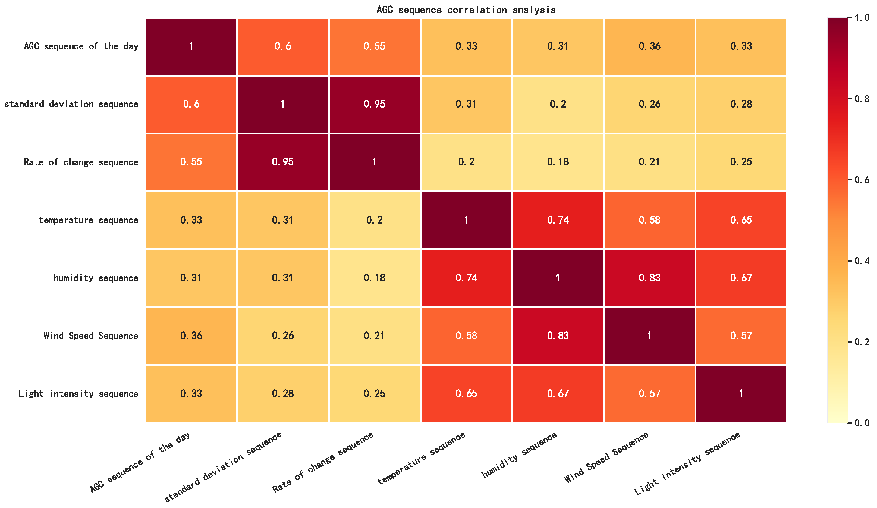
3.2. Data Correlation Analysis

To achieve the objective of reserve refinement analysis, the load curve for the entire day is divided into 96 segments with a 15-min interval. The following steps are performed for each segment of the load curve to obtain the AGC reserve capacity demand curve consisting of 96 points for the entire day.

(1)

Using actual loads that comply with Shannon’s sampling theorem as raw data inputs.

(2)

The time-domain signal is converted to the frequency domain according to Equation (1).

(3)

Determine the spectral classification corresponding to the AGC reserve according to the frequency domain segmentation criteria and zero out any other spectral information that does not belong to this frequency segmentation.

(4)

Calculate the AGC reserve capacity at that time scale using Equation (5).

The AGC reserve capacity series is separated from the load series, but it exhibits significantly different data characteristics compared to the load sequence. The AGC reserve capacity series displays overall higher volatility and larger peak-to-valley differences. In contrast, the load series demonstrates a cyclical pattern over time with no significant abrupt changes in load values between adjacent time periods. However, the AGC reserve series lacks this cyclical pattern and exhibits noticeable jumps between the data in adjacent time periods.

According to existing experience [57], the AGC reserve capacity demand is closely related to the fluctuation component of the load. The periods of high AGC reserve capacity roughly coincide with the periods of significant load variations. Here, the load’s phase fluctuation standard deviation $s_T$ and phase change rate $m_T$ are introduced, as shown in the following Equation (9):

$$s_T=\sqrt{\frac{1}{K}\sum _{i=1}^K{\left|L_i-u_T\right|}^2}$$

(9)

$$m_T=\frac{L_1-L_K}{T_{time}}$$

(10)

In the above Equation (9), K is the total number of load sampling points in time period T, $L_i(i=1,2,\dots ,K)$ is the number of load sampling points in time period T, $T_{time}$ is the duration of time period T in minutes. Here, taking the length of time period T as 15 min and calculating it every 15 min will result in a sequence of load fluctuation standard deviation and a sequence of load rate of change for 96 points in a day.

Since meteorological factors such as temperature, humidity, sunshine, wind speed, etc., have an impact on people’s daily lives and consequently affect the magnitude of the load, we collected meteorological data and computed their average values every 15 min. The recorded data include the average temperature sequence, average humidity sequence, average light intensity sequence and average wind speed sequence for a day. In this study, we take the example of the AGC reserve capacity demand sequence of a province in southern China on 20 July 2018. We employ the maximum mutual information coefficient method to perform correlation analysis between the aforementioned influencing factor sequences. The calculation results are depicted in Figure 3 below.

From Figure 3, the MIC values for meteorological factors such as temperature, humidity, wind speed and light intensity were small, indicating weak correlations (less than 0.5) with the AGC reserve capacity demand sequence. On the other hand, the load curve’s inherent characteristics, such as fluctuation variance and rate of change, exhibited large MIC values, all greater than 0.5, indicating strong correlations with the AGC reserve capacity demand sequence of the day.

In actual forecasting scenarios, the input characteristic data can only consist of historical daily data. Therefore, the maximum mutual information coefficient (MIC) is utilized to calculate the relationship between the AGC reserve capacity demand sequence on 20 July 2018 and the sequences of fluctuation variance and rate of change, which exhibit significant correlation coefficients, as depicted in Figure 3. Since the trend of daily load fluctuation curves is generally consistent, the AGC reserve capacity sequences from historical days also provide informative insights. The specific correlation coefficients are presented in

Table 2. Correlation coefficient between daily AGC reserve demand series and historical daily characteristic data.

Sample Inputs	Correlation Coefficient	Sample Inputs	Correlation Coefficient	Sample Inputs	Correlation Coefficient
${\mathrm{A}}^{-10}$	0.4232	${\mathrm{S}}^{-10}$	0.3012	${\mathrm{M}}^{-10}$	0.2878
${\mathrm{A}}^{-9}$	0.4715	${\mathrm{S}}^{-9}$	0.3530	${\mathrm{M}}^{-9}$	0.3029
${\mathrm{A}}^{-8}$	0.5068	${\mathrm{S}}^{-8}$	0.3919	${\mathrm{M}}^{-8}$	0.3554
${\mathrm{A}}^{-7}$	0.6771	${\mathrm{S}}^{-7}$	0.5403	${\mathrm{M}}^{-7}$	0.5021
${\mathrm{A}}^{-6}$	0.5524	${\mathrm{S}}^{-6}$	0.4238	${\mathrm{M}}^{-6}$	0.3969
${\mathrm{A}}^{-5}$	0.6311	${\mathrm{S}}^{-5}$	0.4997	${\mathrm{M}}^{-5}$	0.3630
${\mathrm{A}}^{-4}$	0.5844	${\mathrm{S}}^{-4}$	0.4552	${\mathrm{M}}^{-4}$	0.4076
${\mathrm{A}}^{-3}$	0.6584	${\mathrm{S}}^{-3}$	0.4336	${\mathrm{M}}^{-3}$	0.4271
${\mathrm{A}}^{-2}$	0.6831	${\mathrm{S}}^{-2}$	0.5359	${\mathrm{M}}^{-2}$	0.5331
${\mathrm{A}}^{-1}$	0.6919	${\mathrm{S}}^{-1}$	0.5709	${\mathrm{M}}^{-1}$	0.5429

below. In Table 2, $\mathrm{A}$ represents the sequence of AGC reserve capacity demand on a historical day, $\mathrm{S}$ represents the sequence of load fluctuation standard deviation on a historical day, $\mathrm{M}$ represents the sequence of load rate of change on a historical day, and the numbers indicate the number of days between historical days.

As shown in Table 2 below, the current day’s AGC reserve capacity demand sequence exhibits a high correlation with the AGC reserve capacity demand sequence from historical days as well as the load standard deviation sequence and load change rate sequence from historical days. Therefore, the load fluctuation standard deviation, load change rate and AGC reserve capacity demand sequence from historical days are selected as inputs for the neural network.

4. IWOA-Attention-BiLSTM Modeling

4.1. Bilstm Network

Long short-term memory neural networks (LSTM), as an improved type of recurrent neural network (RNN), effectively addresses the challenge of long-term dependencies. BiLSTM (bidirectional LSTM) further enhances LSTM by incorporating two LSTM layers with the same structure but in opposite directions. This architecture enables the model to better capture time-series information, and the network structure expression for BiLSTM is provided below:

$${\overrightarrow{h}}_t=\mathrm{LSTM}\left(x_t,{\overrightarrow{h}}_{t-1}\right)$$

(11)

$${\overleftarrow{h}}_t=\mathrm{LSTM}\left(x_t,{\overleftarrow{h}}_{t-1}\right)$$

(12)

$$h_t=W_{{\overrightarrow{h}}_t}{\overrightarrow{h}}_t+W_{{\overleftarrow{h}}_t}{\overleftarrow{h}}_t+b_t$$

(13)

In the above Equations (11) and (12), LSTM is the above traditional LSTM neural network operation process. In the above Equation (13), $W_{\overleftarrow{h}}$ and $W_{\overrightarrow{h}}$ are the forward hidden layer and backward hidden layer weight matrices at time t, respectively; ${\overrightarrow{h}}_t$ and ${\overleftarrow{h}}_t$ are the forward hidden layer and backward hidden layer state vectors at time t, respectively; b_t is the bias of the hidden layer state at moment t.

From the network structure of BiLSTM, it can be seen that the output $h_t$ of the hidden layer at the moment t is a splicing of the processing results in both directions, which contains the complete past and future information in the spare capacity feature data $x_t$. Moreover, the weights are shared during the training process, which ensures its generalization ability while continuously increasing the data volume.

4.2. Attention Mechanism

The attention mechanism is a resource allocation mechanism that characterizes the importance that the temporal target attaches to the input information x at moment t by calculating the attention weight $a_t$ of that information [58,59,60]. If $x^m(m=1,2,\dots ,M)$ is the feature input of the attention mechanism; $h_{t-1}$ and $s_{t-1}$ are the hidden layer state and the gating unit state at the previous moment of the LSTM; and $e_t^m(m=1,2,\dots ,M)$ is the attention weight of each relevant feature at the current moment t, which can be expressed as follows:

$$e_t^m=V_e^{\mathrm{T}}tanh\left(W_e\left[h_{t-1};s_{t-1}\right]+U_e{x}^m+b_e\right)$$

(14)

In the above Equation (14), $V_e$, $W_e$, $U_e$ and $b_e$ are the multilayer perceptron weights and bias parameters for calculating the attention weights. $a_t^m(m=1,2,\dots ,M)$ is for is the feature weights after normalization using the softmax function, which can be expressed as follows:

$$a_t^m=softmax\left(e_t^m\right)=\frac{exp\left(e_t^m\right)}{{\sum }_{i=1}^{M}exp\left(e_t^i\right)}$$

(15)

The associated characterization matrix of the AGC reserve capacity demand sequence is represented as follows:

$$X=\left[\begin{array}{cccc}{x}_1^1& x_2^1& \cdots & x_M^1\\ x_1^2& x_2^2& \cdots & x_M^2\\ x_1^3& x_2^3& \cdots & x_M^3\end{array}\right]$$

(16)

In the above Equation (16), $x^i=(x_1^1,x_2^1,\dots ,x_M^1)$ is the value of the relevant characterizing factor at M historical moments. More specifically, $x^1$, $x^2$ and $x^3$ are the historical daily AGC reserve capacity demand sequence, the historical daily load fluctuation standard deviation sequence and the historical daily load change rate sequence. The eigenvalue $a_t^m$ obtained from normalization is multiplied with $x_i^m$ to obtain the new eigenvalue $\widetilde{x_t}$ to enhance or weaken the features of type m. The expression of $\widetilde{x_t}$ is shown below:

$$\widetilde{x_t}={\left({\alpha }_t^1{x}_t^1,{\alpha }_t^2{x}_t^2,\cdots ,{\alpha }_t^M{x}_t^M\right)}^{\mathrm{T}}$$

(17)

4.3. Improved Whale Algorithm

To overcome the limitations of the traditional classical whale algorithm, which is prone to local optimization and premature convergence, this paper proposes a multi-strategy improvement approach for the traditional whale optimization algorithm (WOA). The proposed approach encompasses three key enhancements. Firstly, the population initialization is performed using the Sobol sequence. Secondly, the original linear convergence factor is improved. Lastly, adaptive weighting coefficients are incorporated into the WOA.

Utilizing Sobol sequences for the initialization of whale populations can lead to the production of highly uniformly distributed particles, resulting in improved population diversity. The process of generating initial populations using Sobol sequences is as follows:

$$u_i=u_{min}+\lambda (u_{max}-u_{min})$$

(18)

In the above Equation (18), $u_{max}$ and $u_{min}$ are the upper and lower bounds of the initial population position, respectively, $\lambda$ is a random number in the range $[0, 1]$ generated by the Sobol sequence and $u_i$ is the initial position of the ith whale in the population.

The convergence factor a in the classical WOA algorithm linearly decreases from 2 to 0, which makes it prone to becoming trapped in local optima. To overcome this limitation, a nonlinear inverse tangent convergence factor is introduced. Its mathematical model is expressed as follows:

$$a=2-\frac{4}{\pi }arctan\left(\frac{10t}{t_{max}}\right)$$

(19)

In the above Equation (19), t represents the number of iterations and $t_{max}$ represents the maximum number of iterations.

Meanwhile, drawing on the concept of weights, adaptive weights $\omega$ are introduced to refine the position updating process in the three stages of whale contraction encircling, upward spiraling and prey searching. During the early stage, larger adaptive weights are utilized to favor global search, while smaller weights are employed toward the end of the iterative process to enhance the whale group’s ability for local exploitation. The mathematical expression for adaptive weighting is as follows:

$$\omega =sin\left(\frac{\pi t}{2t_{max}}+\pi \right)+1$$

(20)

After the introduction of adaptive weights, the positional formulas of WOA in each of the three phases of contraction encirclement, upward spiral and prey search are updated as follows:

$$\overrightarrow{X}(\tau +1)=\omega \overrightarrow{X}{}^{\ast }\left(\tau \right)-A·\overrightarrow{D}$$

(21)

$$\overrightarrow{X}(\tau +1)=\omega {\overrightarrow{D}}^{\prime }·e^{bl}·cos\left(2\pi l\right)+\overrightarrow{X}{}^{\ast }\left(\tau \right)$$

(22)

$$\overrightarrow{X}(\tau +1)=\omega {\overrightarrow{X}}_{rand}\left(\tau \right)-A·{\overrightarrow{D}}_{rand}$$

(23)

In the above Equations (21)–(23), $\tau$ represents the number of iterations, $\overrightarrow{X}{}^{\ast }\left(\tau \right)$ represents the optimal position of the $\tau$th iteration in the pod, A represents the coefficient phase quantity, $\overrightarrow{D}$ and ${\overrightarrow{D}}^{\prime }$ represent the distance to the whales at the optimal position in the pod, ${\overrightarrow{D}}_{rand}$ represents the distance to a randomly selected whale in the pod, b represents the constant of the logarithmic helix equation, l represents a random number between [−1, 1] and ${\overrightarrow{X}}_{rand}$ represents the position of any randomly selected individual in the pod.

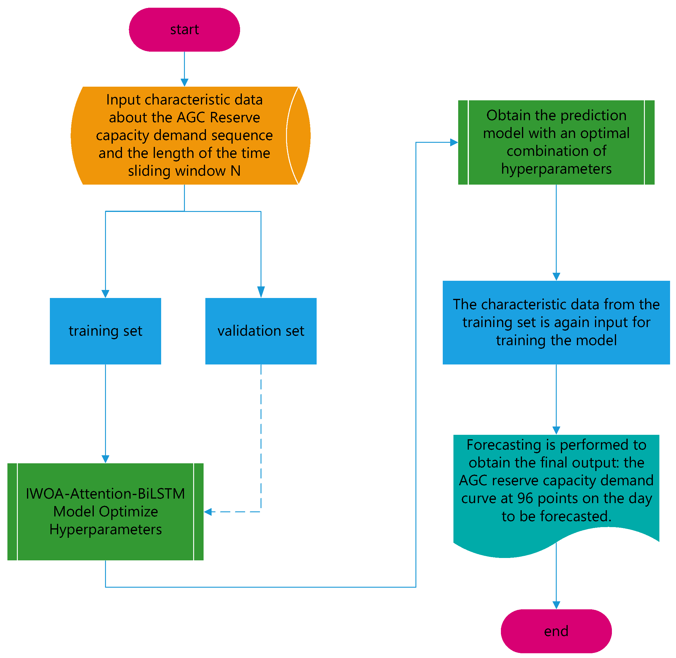
4.4. IWOA-Attention-BiLSTM Model Design and Forecasting Process

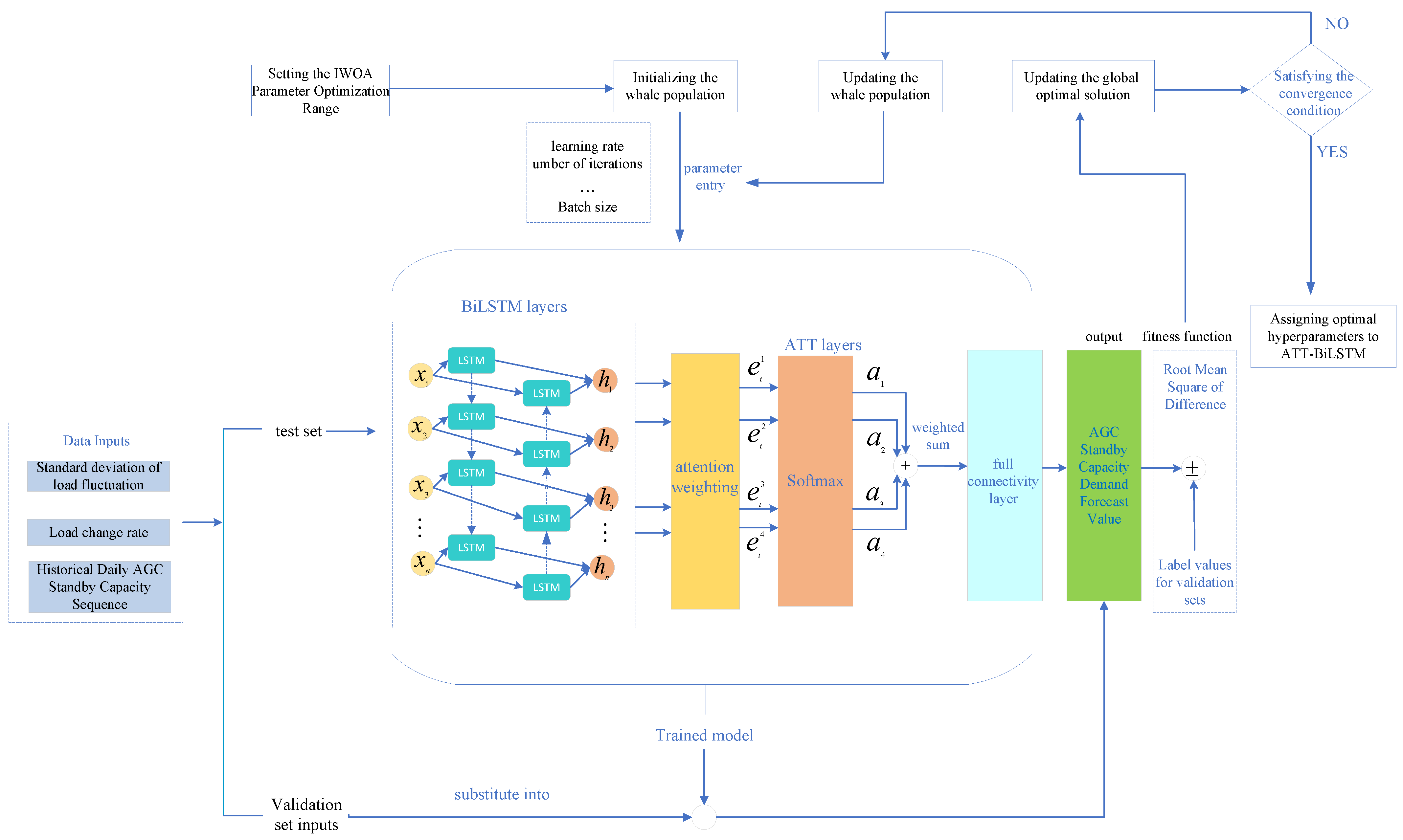
The BiLSTM model incorporates several hyperparameters, including the number of input and output layers, which align with the dimensions of the input and output data. Additionally, hyperparameters such as the initial learning rate $\eta$, the number of neurons in the hidden layer m, the number of iterations H, the batch size k (i.e., number of samples selected for each training session) and the number of neurons in the fully connected layer l all have a significant impact on the model’s accuracy and efficiency. In this study, the Attention-BiLSTM model is optimized using the improved whale algorithm IWOA to fine-tune these hyperparameters. The optimization process aims to enhance the model’s prediction performance by utilizing prediction accuracy as the fitness function.

The fitting function used in this optimization is the minimization of the root-mean-square (RMS) value between the predicted output values and the true values of the test set. The position coordinates of each whale are located within a high-dimensional space, encompassing hyperparameters such as the initial learning rate $\eta$, the number of neurons in the hidden layer m, the number of iterations H, the batch size k (i.e., the number of samples selected for each training session) and the number of neurons in the fully connected layer l. During each iteration of the whale algorithm, the fitness of each whale is calculated, and the individual optimal position and group optimal position are updated, subsequently. The iterative process continues until the optimal hyperparameter values are achieved.

The overall forecasting processes is shown in Figure 4. The characteristic data about the AGC reserve capacity demand sequence include a 96-point sequence of load fluctuation standard deviation, 96-point sequence of load change rate and 96-point sequence of AGC reserve capacity demand sequence from historical days. As shown in Section 3.2, their correlation coefficients are even larger. So the input data include the sequence associated with the AGC reserve capacity in three dimensions, and the dimensions of the input data are $N\times 96\times 3$. The output data are the sequence of AGC reserve capacity demand at 96 points on the day to be forecasted. The IWOA-Attention-BiLSTM hyperparameter optimization model is shown in Figure 5 below.

In Figure 5, the hyperparameter optimization search step is shown below:

(1)

Setting the whale population size, search space dimension, maximum number of iterations and the Attention-BiLSTM hyperparameters for the optimization range to achieve the initialization of the whale population;

(2)

Calculating and recording the optimal fitness of each whale group under the current hyperparameters;

(3)

Constant updating of individual whale positions and optimization of hyperparameters;

(4)

Comparing the fitness of the new position of the whale; if the new value is better than the current optimal value, update the individual optimal fitness of the whale group, if the current value is still better than the new value, keep it unchanged and continue training;

(5)

Determining whether the termination condition is met; if it is met, the optimal hyperparameters are given to Attention-BiLSTM; if not, return to (3);

(6)

Using the optimized hyperparameters to build a load day-ahead AGC reserve capacity demand forecasting model and perform load day-ahead AGC reserve capacity demand forecasting.

4.5. Selection of Evaluation Indicators

In this paper, the mean absolute percentage error ($MAPE$), the root mean square error ($RMSE$) and the coefficient of certainty ($R^2$) are selected as the evaluation indexes of the prediction model. The formula is as follows:

$$MAPE=\frac{1}{N}\sum _{i=1}^N\left|\frac{{\widehat{y}}_i-y_i}{y_i}\right|\times 100\%$$

(24)

$$RMSE=\sqrt{\frac{1}{N}\sum _{i=1}^N{({\widehat{y}}_i-y_i)}^2}$$

(25)

$$R^2=1-\frac{{\displaystyle \sum _{i=1}^N}{(y_i-{\widehat{y}}_i)}^2}{{\displaystyle \sum _{i=1}^N}{(y_i-y_{ave})}^2}$$

(26)

In the above Equations (24)–(26), N represents the total number of predicted outcomes; ${\widehat{y}}_i$ is the predicted value at point i in the AGC reserve capacity demand sequence; $y_i$ is the actual value at point i in the AGC spare capacity demand sequence; $y_{ave}$ is the forecast mean of the AGC reserve capacity demand sequence; $MAPE$ is expressed in percentage, $RMSE$ is expressed in megawatts, and $R^2$ has no unit.

5. Case Study

5.1. Preprocessing of Reserve Capacity Data

In this paper, we use the real load data of a specific province in China’s southern power grid. The dataset spans a period of 1461 days, from 1 January 2018 to 31 December 2021. The load data were sampled at a frequency of 30 s, resulting in 2880 data points per day. Overall, the dataset contains a total of 4,207,680 data points, representing the load measurements over the entire four-year period.

Using a smaller sampling interval increases the likelihood of encountering abnormal load data, which may lead to fluctuations in AGC reserve capacity calculation values. In this study, a weekly optimization cycle is employed to mitigate the impact of abnormal data. Specifically, the AGC reserve calculation values at the same moment within the same week are filtered using the following formula:

$$\frac{\left|R_{i,t}-R_{ave,t}\right|}{R_{ave,t}}\times 100\%\le 90\%$$

(27)

In the above Equation (27), $R_{i,t}$ is the calculated value of AGC reserve capacity under moment t on day i of the week and $R_{ave,t}$ is the calculated value of average AGC reserve capacity under moment t of the week. If Equation (27) is not satisfied, then the AGC reserve is large or small. In this paper, we use the average value $R_{ave,t}$ of the same moment to replace these values.

The preprocessed reserve capacity demand calculation data for 16 February 2018 (Spring Festival), 24 June 2018 (regular weekend) and 12 December 2018 (regular weekday) are shown below.

As can be seen from Figure 6 above, most of the spikes in the AGC reserve capacity sequence occur during load rise or load fall periods such as 5:00 a.m. to 7:00 a.m., 8:00 a.m. to 9:00 a.m., 11:00 p.m. to 13:00 p.m., 16:00 p.m. to 17:00 p.m. and 22:00 p.m. to 23:00 p.m. As mentioned before, the AGC reserve is mainly used to cope with load components with change periods between tens of seconds and minutes such as electric furnaces, calendering machines, electric locomotives and other industrial load fluctuations with shocks. The above time periods also correspond to the time periods of the day when factories are in operation, on lunch breaks and out of operation. The values of reserve capacity demand on the Chinese New Year and ordinary weekends are smaller than those on weekdays and the fluctuations of the demand curves are also smaller. This is due to the fact that on weekends and holidays, there is a certain degree of factory shutdowns compared to weekdays. The proportion of shock loads such as electric furnaces, calendering machinery and electric locomotives decreases, resulting in smaller load fluctuations on a second-to-minute scale. It can be seen that the method of using spectrum analysis is not only feasible in principle, but the calculation results are also in line with the actual situation.

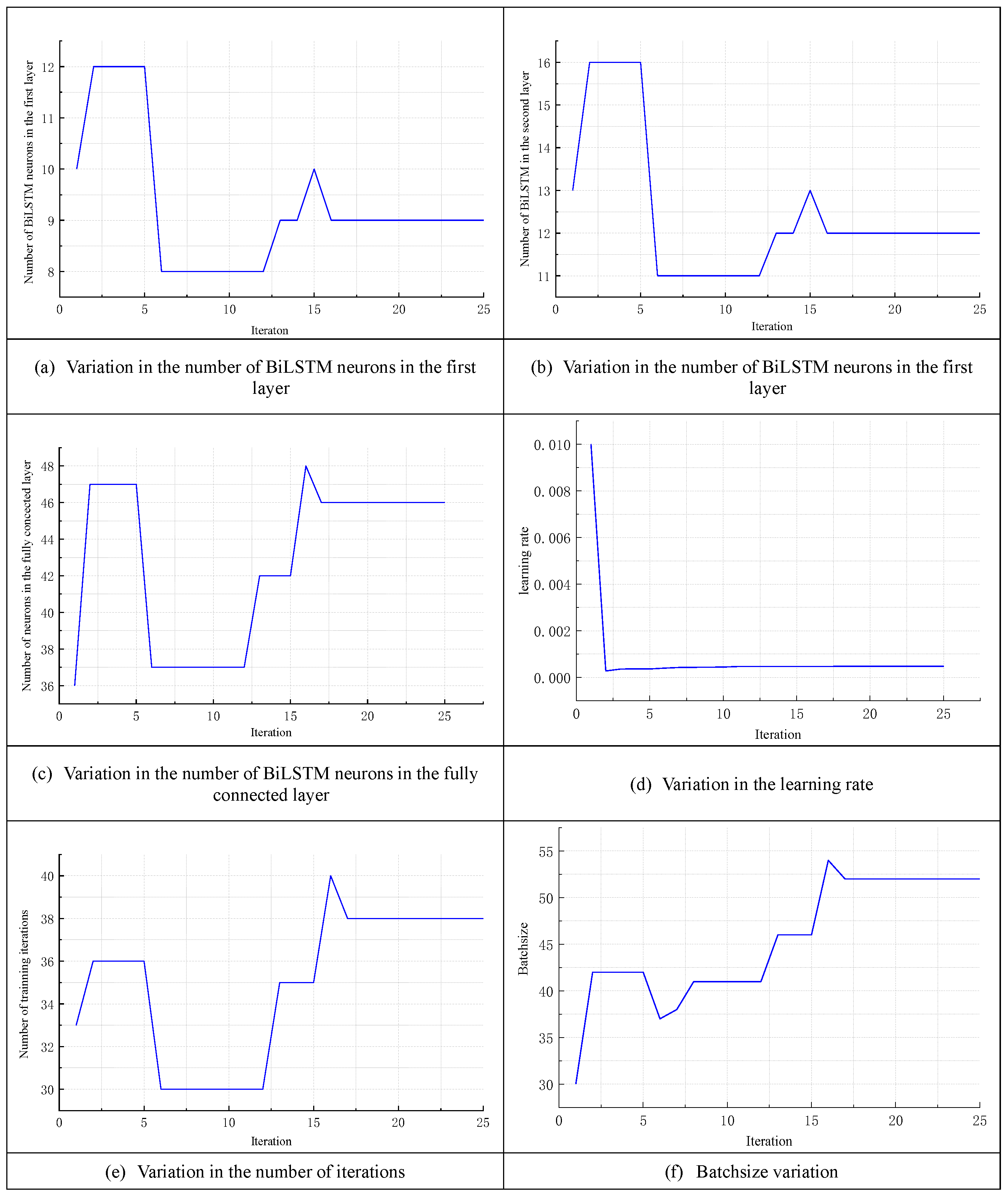
5.2. Model Structure and Hyperparameter Optimization

All the simulation experiments in this paper are based on the Windows 10 operating system, the CPU is an Intel Core i7-10700, 2.90 GHz, the software is Python 3.7.0 and the framework is Tensorflow 2.2.0. To fully utilize the daily cycle characteristic of the loads and the weekly cycle characteristic, this section adopts the length of the time-sliding window of 7, i.e., the input data are the 96-point AGC spare capacity sequence, the 96-point load fluctuation standard deviation sequence and the 96-point load change rate sequence for the 7 days before the day to be forecast. The output data are the 96-point AGC spare capacity demand on the day to be forecasted. The structural parameters of the model using the Attention-BiLSTM neural network are shown in

Table 3. Attention-BiLSTM predicts model parameters.

Parameter Name	Parameter Value	Parameter Name	Parameter Value
Dimension of input features	7 × 96 × 3	Learning rate	awaiting optimization
Number of neurons in the input layer	288	Number of training iterations	awaiting optimization
Number of BiLSTM neurons in the first layer	awaiting optimization	Batchsize	awaiting optimization
Number of BiLSTM neurons in the second layer	awaiting optimization	Number of neurons in the output layer	96
Number of neurons in the fully connected layer	awaiting optimization	/	/

.

The parameter optimization process is shown in Figure 7 below, and the final hyperparameter optimization results obtained are shown in

Table 4. Model hyperparameter optimization results.

Hyperparameterization	Setting Range	Post-Optimization
Number of BiLSTM neurons in the first layer	[10, 100]	9
Number of BiLSTM neurons in the second layer	[10, 100]	12
Number of neurons in the fully connected layer	[10, 100]	46
learning rate	[0.0001, 0.01]	0.000476
Number of training iterations	[10, 100]	38
Batchsize	[16, 128]	52

below.

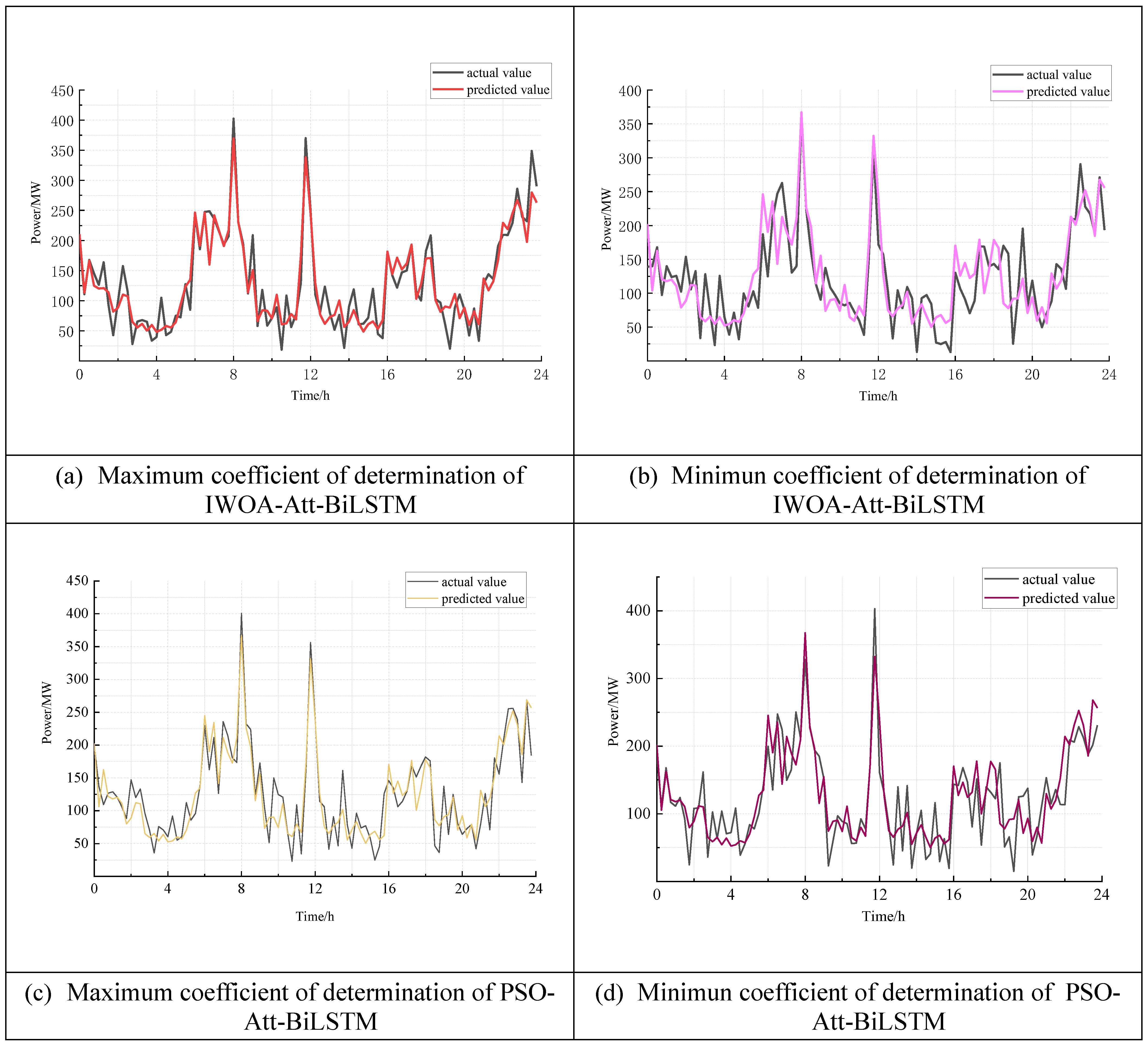
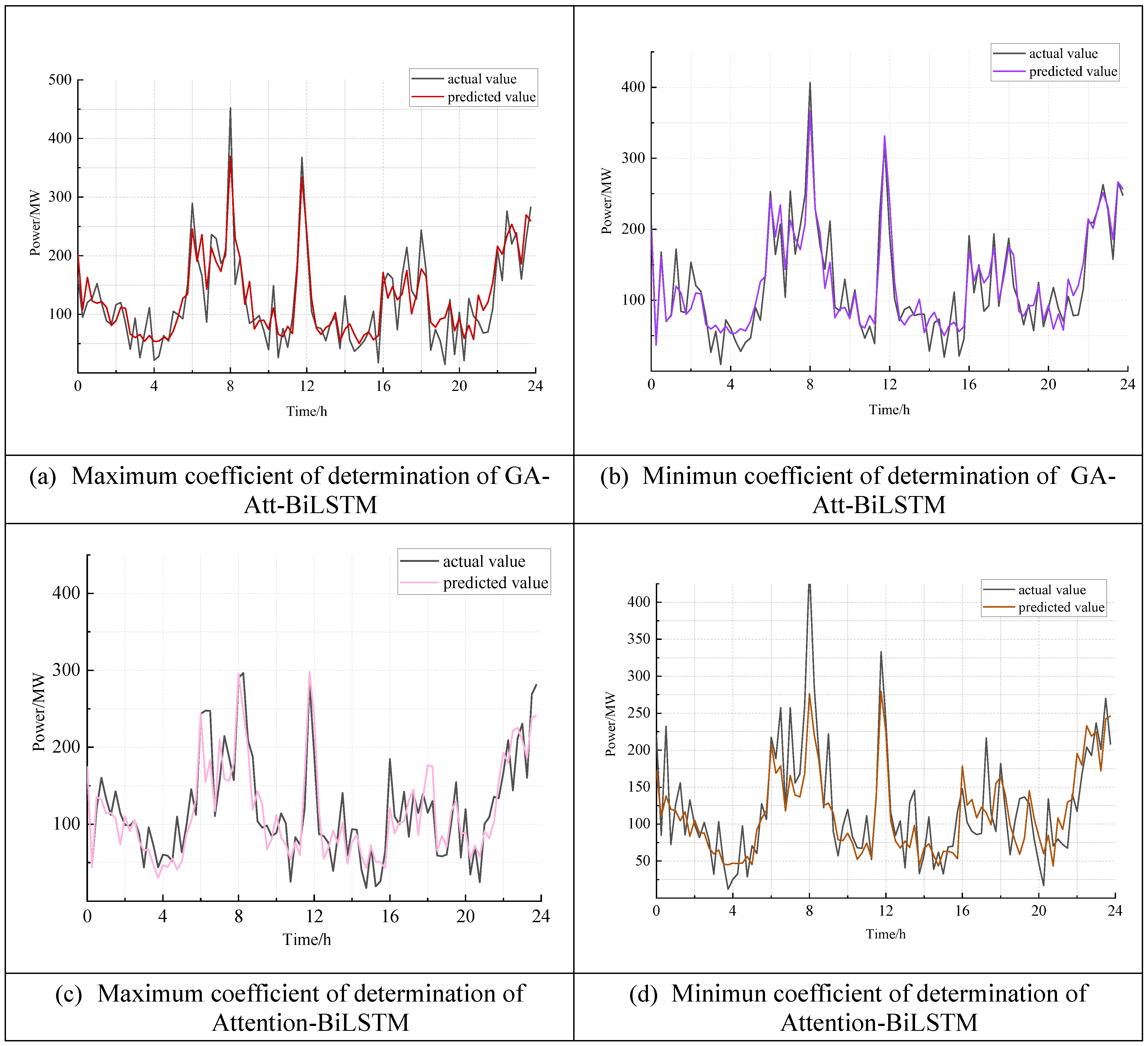
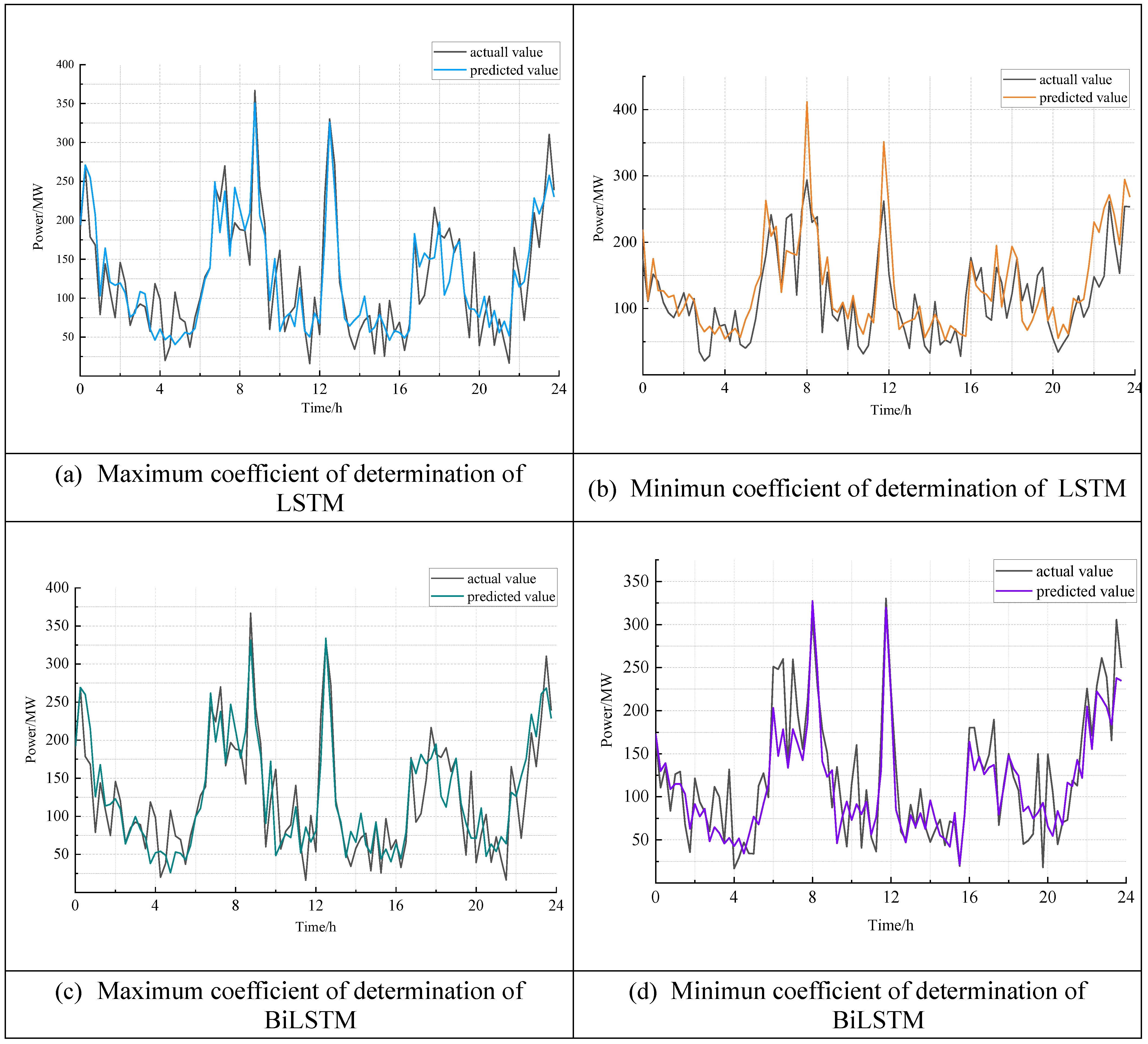
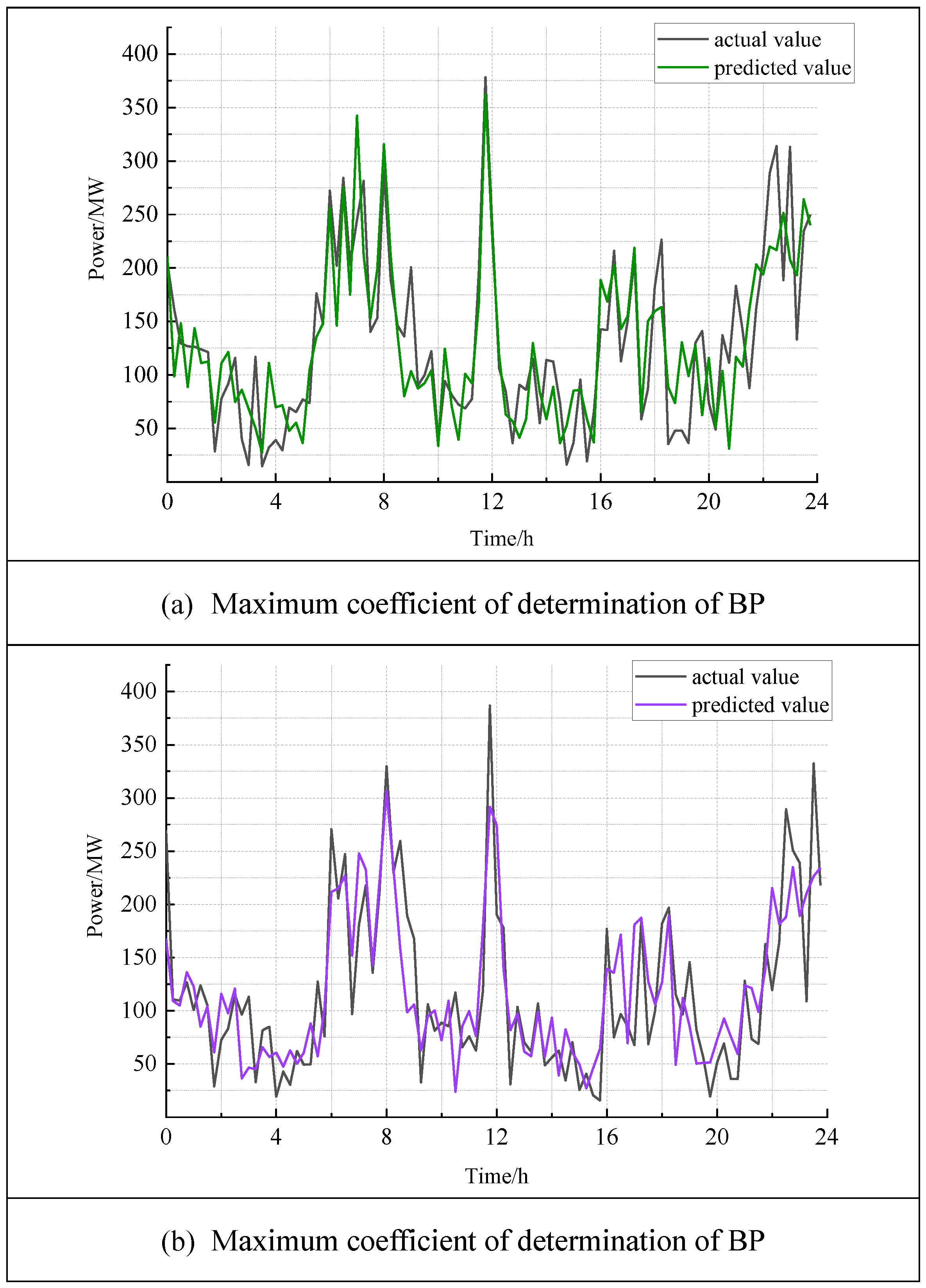
5.3. Load AGC Reserve Capacity Demand Forecast

In this paper, a BiLSTM network with two hidden layers is utilized and the hyperbolic tangent (tanh) function is employed as the activation function. The abstract information extracted from the Attention-BiLSTM network is nonlinearly mapped through a fully connected layer and outputted using the Rectified Linear Unit (ReLU) function. The AGC reserve capacity demand for load forecasting is predicted using the Attention-BiLSTM network with optimized hyperparameters obtained from the improved whale optimization algorithm (IWOA). The training set consists of load AGC reserve capacity and related feature data from a province in southern China, spanning 30 months from January 2018 to June 2021. The test set comprises load AGC reserve capacity data for 6 months from July to December 2021.

Table 5. Prediction accuracy of different models in the second half of 2021.

Categories	Criteria	Prediction Model
		LSTM	BiLSTM	BP	Att-BiLSTM	GA-Att-BiLSTM	PSO-Att-BiLSTM	IWOA-Att-BiLSTM
each mo- nth	$MAPE/\%$	33.9	33.4	38.1	33.2	33.6	32.9	32.6
	$RMSE$/MW	34.5	33.9	40.6	34.0	33.2	33.5	32.2
	$R^2$	0.772	0.775	0.689	0.780	0.792	0.784	0.804
half year	$MAPE$/%	33.5	33.0	38.1	33.2	32.9	32.8	32.6
	$RMSE$/MW	33.9	34.5	40.6	34.2	33.2	33.1	32.2
	$R^2$	0.775	0.776	0.690	0.781	0.788	0.797	0.805

presents a comparison of the prediction model proposed in this paper with four other models, namely back-propagation neural network (BP), long short-term memory neural network (LSTM), bidirectional long short-term memory neural network (BiLSTM) and Attention-BiLSTM. In addition, since particle swarm algorithms (PSOs) and genetic algorithms (GAs) can also be used for hyperparameter optimization [61], the prediction model in this paper is also compared with PSO-Attention-BiLSTM model and GA-Attention-BiLSTM, and the range of hyperparameter settings is the same for all three optimization models. Table 5 showcases the prediction averages for the six-month period and the overall prediction results for the second half of the year.

As shown in Table 5, the IWOA-Attention-BiLSTM model has the best average prediction results in each month and the overall prediction results of the test set. Analyzing from the perspective of the average prediction results in each month, the prediction accuracy of the proposed model in this paper is the highest compared to the other six models. The $MAPE$ is reduced by 3.83%, 2.46%, 14.57%, 1.89%, 2.97% and 0.92% compared to the other six models, and the $RMSE$ is reduced by 6.55%, 4.95%, 20.58%, 5.23%, 3.01% and 3.89% compared to the other six models. The $R^2$ is improved by 3.98%, 3.61%, 20.59%, 3.03%, 1.52% and 2.55%, respectively, compared with the other six models. Analyzing from the perspective of the overall prediction effect of the test set, the prediction model proposed in this paper also has obvious superiority compared with the other six models. The $MAPE$ is reduced by 2.86%, 1.22%, 14.56%, 1.90%, 0.92% and 0.61%, respectively, and the $RMSE$ is reduced by 4.79%, 6.09%, 20.59%, 5.69%, 3.01% and 2.72%, respectively, compared with the other six models; $R^2$ was improved by 3.89%, 3.54%, 16.53%, 3.01%, 2.16% and 1.00%, respectively, compared to the other six models.

The test set spans 184 days from 1 July to 31 December.

Table 6. The maximum value of certainty coefficient and corresponding days of different AGC reserve capacity demand forecasting models.

Categories	LSTM	BiLSTM	BP	Att-BiLSTM	GA-Att-BiLSTM	PSO-Att-BiLSTM	IWOA-Att-BiLSTM
maximum value of $R^2$	0.8732	0.8546	0.8434	0.8542	0.8762	0.8748	0.8810
correspon- ding date	17 October	17 October	8 December	5 August	26 December	15 September	29 December
minimum value of $R^2$	0.5994	0.5936	0.4512	0.6664	0.6533	0.6542	0.6651
correspon- ding date	1 August	11 October	21 September	11 August	8 July	7 December	18 July

presents the maximum value of the certainty coefficient ($R^2$) achieved by each model along with its corresponding date. Furthermore, Figure A1, Figure A2, Figure A3 and Figure A4 in Appendix A show the forecast effect on the forecast days with the maximum and minimum certainty coefficients for the different models mentioned above. Additionally, Figure 8 displays the calculation results of the certainty coefficient evaluation index ($R^2$) for each day of every prediction model, the daily mean absolute percentage error ($MAPE)$ evaluation index of each prediction model in the test set is calculated in Figure 9, and the root mean square error ($RMSE$) evaluation index calculation results of each prediction model in the test set are shown in Figure 10.

Upon examining Table 6 and Figure 8, Figure 9 and Figure 10, it is evident that the IWOA-Attention-BiLSTM model demonstrates superior predictive stability compared to the other six models, as indicated by wider upper and lower bounds on the coefficient of determination and had the lowest levels of MAPE and RMSE. In terms of overall prediction effectiveness, the IWOA-Attention-BiLSTM model consistently achieves a higher coefficient of certainty for the majority of reserve prediction days in the test set, outperforming the other six prediction models. Furthermore, Figure A1 in Appendix A reveals that the IWOA-Attention-BiLSTM model accurately captures the sharp peak of reserve demand for both the best and worst predicted days. This observation suggests that the attention mechanism effectively focuses on important feature points, assigning larger weight coefficients.

6. Conclusions

In this paper, the method of spectrum analysis is employed to refine the distinction between various types of load reserve capacity by utilizing response time as a criterion. The Attention-BiLSTM network model, optimized using the improved whale optimization algorithm (IWOA), is employed to forecast the AGC reserve capacity demand before the load day, resulting in improved accuracy and predictive capabilities. The characteristics of the IWOA-Attention-BiLSTM method are as follows:

(1)

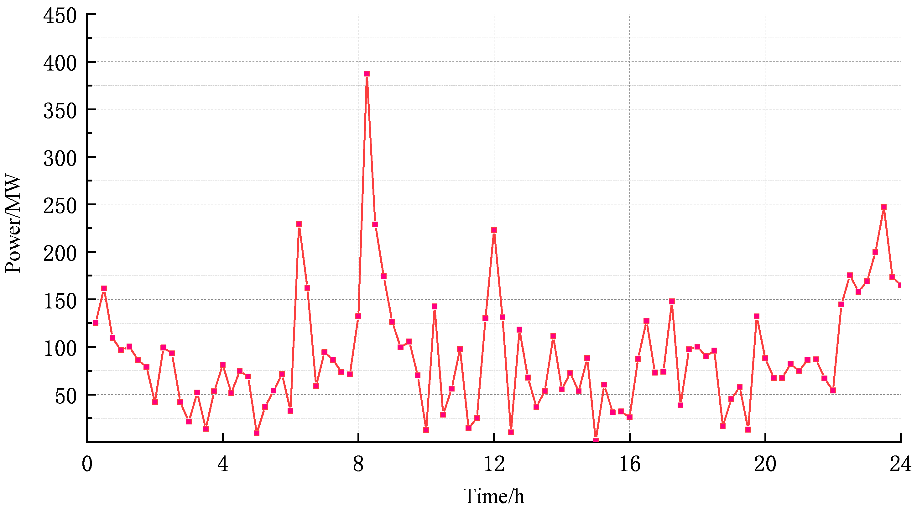
With the goal of fine-grained analysis of reserve demand, the load curves are decomposed using Fourier transform at a finer time scale. This, combined with Parseval’s theorem, enables the extraction of load AGC reserve demand curves for sub-times of the day, effectively supporting curve-level reserve forecasting.

(2)

By comparing the load AGC reserve capacity demand curve with the load curve, the maximum mutual information coefficient method quantifies the relationship between the fluctuating characteristics of the load curve and the load AGC reserve capacity demand. This information is then used to integrate the historical daily AGC reserve capacity sequence and the historical daily load fluctuating characteristics sequence as inputs to the forecasting model, enhancing its accuracy and predictive capabilities.

(3)

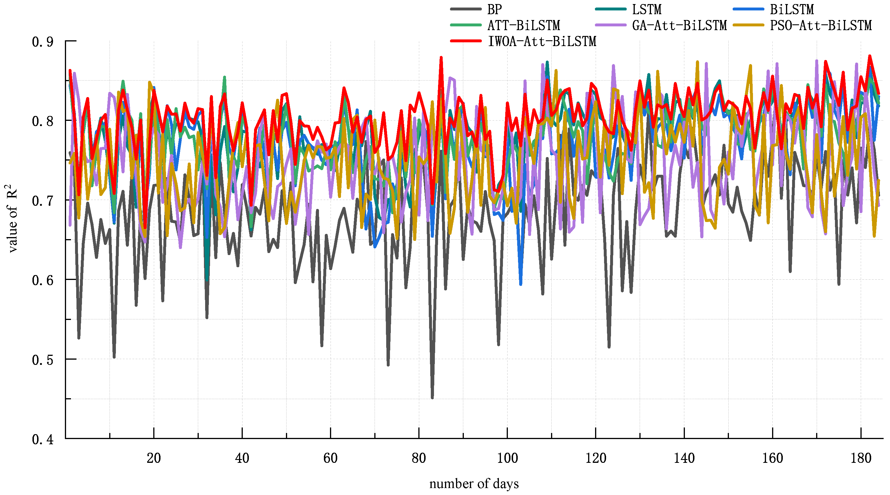
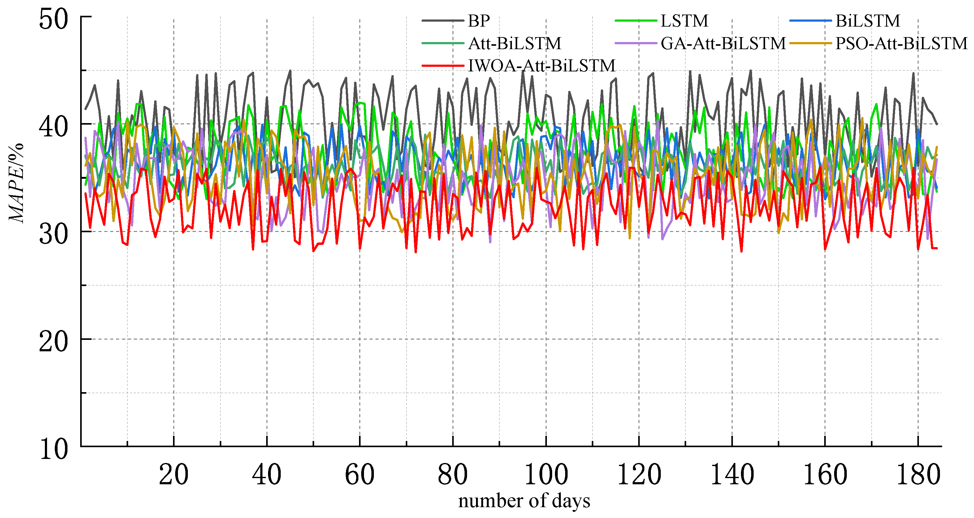
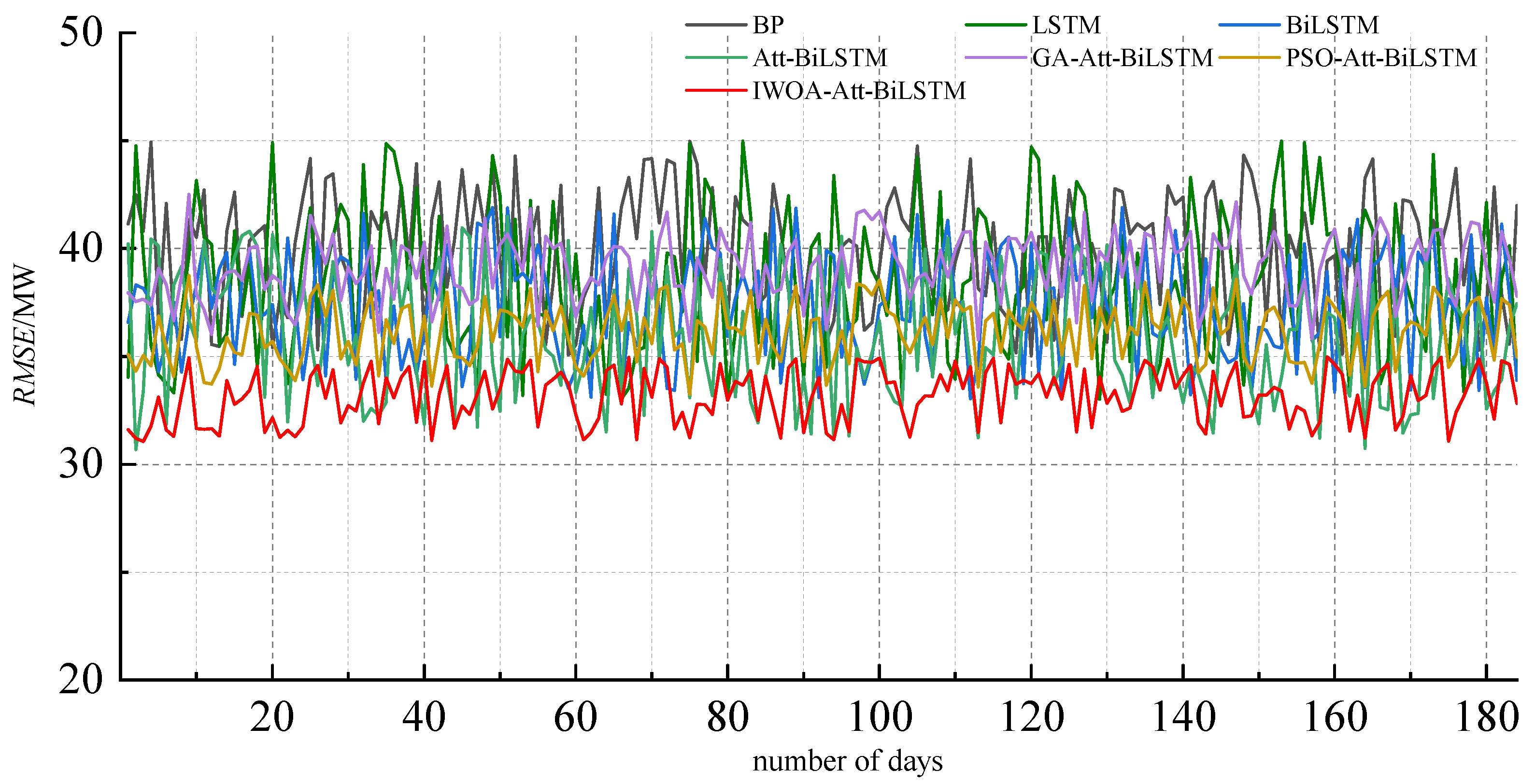
The improved whale optimization algorithm automatically optimizes the hyperparameters of the Attention-BiLSTM model, eliminating the limitations of manual parameter tuning. This optimization leads to improved accuracy in model predictions. Comparisons with other models, such as LSTM, BiLSTM, BP, Attention-BiLSTM, PSO-Attention-BiLSTM and GA-Attention-BiLSTM reveal that the proposed method improves prediction accuracy by 3.89%, 3.54%, 16.53%, 3.01%, 2.16% and 1.00%, respectively. These results highlight the superior predictive capabilities of the models proposed in this paper.

(4)

The main contribution of this paper is that it adopts a more refined method to analyze load reserve on a more refined time scale and combines IWOA-Attention-BiLSTM into a neural network to build a load day-ahead AGC reserve capacity demand prediction model, which can realize the reserve capacity demand prediction of 96 points a day just like load prediction. The predicted results are of guiding significance for AGC demand assessment in the backup auxiliary service market and can also be used for day-ahead scheduling and generation plan designation. According to the predicted results, various types of units can reasonably allocate the AGC reserve demand of the system at various periods, which ensures the safety and stability of the system and at the same time can make more efficient use of various types of power supplies.

In the context of that high percentage of renewable energy access and a further reduction in the system’s hot reserve resources, the forecasting method proposed in this paper is instructive for how to efficiently utilize the existing system resources. The forecasting results can be used for day-ahead scheduling and intra-day monitoring of the generation plan as well as for bidding evaluation in the power reserve market. It should be noted that the load curve we studied is the real sampled load curve, not the net load curve minus the wind and PV output, so the fluctuation of the renewable energy output has no effect on the forecasting method, and subsequent studies can be considered on the basis of the net load curve. In addition, there is still room for improvement in the prediction accuracy of the method proposed in this paper, and subsequent research can decompose the original time series and extract more detailed time-series features to improve the prediction accuracy so as to further improve the significance of the research results for the actual production scheduling.

References

1. Ullah, Z.; Ullah, K.; Diaz-Londono, C.; Gruosso, G.; Basit, A. Enhancing Grid Operation with Electric Vehicle Integration in Automatic Generation Control. Energies 2023, 16, 7118. [Google Scholar] [CrossRef]
2. Ullah, K.; Ullah, Z.; Aslam, S.; Salam, M.S.; Salahuddin, M.A.; Umer, M.F.; Humayon, M.; Shaheer, H. Wind Farms and Flexible Loads Contribution in Automatic Generation Control: An Extensive Review and Simulation. Energies 2023, 16, 5498. [Google Scholar] [CrossRef]
3. Yang, C.; Wu, Z.; Li, X.; Fars, A. Risk-constrained stochastic scheduling for energy hub: Integrating renewables, demand response, and electric vehicles. Energy 2024, 288, 129680. [Google Scholar] [CrossRef]
4. Yao, L.; Wang, Y.; Xiao, X. Concentrated Solar Power Plant Modeling for Power System Studies. IEEE Trans. Power Syst. 2023, 1–12. [Google Scholar] [CrossRef]
5. Yang, M.; Wang, Y.; Xiao, X.; Li, Y. A Robust Damping Control for Virtual Synchronous Generators Based on Energy Reshaping. IEEE Trans. Energy Convers. 2023, 38, 2146–2159. [Google Scholar] [CrossRef]
6. Borunda, M.; Ramírez, A.; Garduno, R.; García-Beltrán, C.; Mijarez, R. Enhancing Long-Term Wind Power Forecasting by Using an Intelligent Statistical Treatment for Wind Resource Data. Energies 2023, 16, 7915. [Google Scholar] [CrossRef]
7. Hao, C.H.; Wesseh, P.K.; Okorie, D.I.; Abudu, H. Implications of Growing Wind and Solar Penetration in Retail Electricity Markets with Gradual Demand Response. Energies 2023, 16, 7895. [Google Scholar] [CrossRef]
8. Finamore, A.R.; Calderaro, V.; Galdi, V.; Graber, G.; Ippolito, L.; Conio, G. Improving Wind Power Generation Forecasts: A Hybrid ANN-Clustering-PSO Approach. Energies 2023, 16, 7522. [Google Scholar] [CrossRef]
9. Benitez, I.B.; Ibañez, J.A.; Lumabad, C.I.D.; Cañete, J.M.; Principe, J.A. Day-Ahead Hourly Solar Photovoltaic Output Forecasting Using SARIMAX, Long Short-Term Memory, and Extreme Gradient Boosting: Case of the Philippines. Energies 2023, 16, 7823. [Google Scholar] [CrossRef]
10. LÜ, M.; Lou, S.; Liu, J.; Wu, Y.; Wang, Z. Coordinated Optimization of Multi-type Reserve in Virtual Power Plant Accommodated High Shares of Wind Power. Proc. CSEE 2018, 38, 2874–2882+3138. [Google Scholar] [CrossRef]
11. Wang, B.; Tang, N.; Fang, X.; Yang, S.; Ji, W. A Multi Time Scales Reserve Rolling Revision Model of Power System With Large Scale Wind Power. Proc. CSEE 2017, 37, 1645–1657. [Google Scholar] [CrossRef]
12. Zhang, X.; Wang, Z.; Lu, Z. Multi-objective load dispatch for microgrid with electric vehicles using modified gravitational search and particle swarm optimization algorithm. Appl. Energy 2022, 306, 118018. [Google Scholar] [CrossRef]
13. Zhao, L.; Zeng, Y.; Li, Y.; Peng, D.; Wang, Y. Coordinated Planning of Power Systems under Uncertain Characteristics Based on the Multilinear Monte Carlo Method. Energies 2023, 16, 7761. [Google Scholar] [CrossRef]
14. Liu, Y.; Su, T.; Qiu, G.; Gao, H.; Liu, J.; Shui, Y. Analytic Deep Learning and Stepwise Integrated Gradients-based Power System Transient Stability Preventive Control. IEEE Trans. Power Syst. 2023, 38, 1771–1774. [Google Scholar] [CrossRef]
15. Liu, Y.; Gao, S.; Qiu, G.; Liu, T.; Ding, L.; Liu, J. A Physics-Informed Action Network for Transient Stability Preventive Control. IEEE Trans. Power Syst. 2023, 38, 1771–1774. [Google Scholar] [CrossRef]
16. Oureilidis, K.; Malamaki, K.-N.; Gallos, K.; Tsitsimelis, A.; Dikaiakos, C.; Gkavanoudis, S.; Cvetkovic, M.; Mauricio, J.M.; Maza Ortega, J.M.; Ramos, J.L.M.; et al. Ancillary services market design in distribution networks: Review and identification of barriers. Energies 2020, 13, 917. [Google Scholar] [CrossRef]
17. Jay, D.; Swarup, K.S. A comprehensive survey on reactive power ancillary service markets. Renew. Sustain. Energy Rev. 2021, 144, 110967. [Google Scholar] [CrossRef]
18. Park, M.-S.; Chun, Y.-H. Introduction of Generator Unit Controller and Its Tuning for Automatic Generation Control in Korean Energy Management System (K-EMS). J. Electr. Eng. Technol. 2011, 6, 42–47. [Google Scholar] [CrossRef]
19. Yang, X.; Wang, N.; Pan, Z.; Meng, L.; Hu, W. Research on auxiliary automatic generator control marketing system in Hebei Grid. In Communications, Signal Processing, and Systems: Proceedings of the 2017 International Conference on Communications, Signal Processing, and Systems, Harbin, China, 14–17 July 2017; Springer: Berlin/Heidelberg, Germany, 2019; pp. 1888–1894. [Google Scholar]
20. Teng, X.; Gao, Z.; Zhu, B.; Wu, J.; Peng, D.; Xu, R.; Zhang, X. Requirements analysis and key technologies for automatic generation control for smart grid dispatching and control systems. Autom. Electr. Power Syst. 2015, 39, 81–87. [Google Scholar]
21. Zhao, X.; Wang, Z.; Wen, F. New framework for forecasting and procuring automatic generation control capacity. J. Zhejiang Univ. Eng. Sci. 2005, 39, 685. [Google Scholar]
22. Torres, M.E.; Colominas, M.A.; Schlotthauer, G.; Flandrin, P. A complete ensemble empirical mode decomposition with adaptive noise. In Proceedings of the 2011 IEEE International Conference on Acoustics, Speech and Signal Processing (ICASSP), Prague, Czech Republic, 22–27 May 2011; pp. 4144–4147. [Google Scholar]
23. Bessa, R.J.; Matos, M.A.; Costa, I.C.; Bremermann, L.; Franchin, I.G.; Pestana, R.; Machado, N.; Waldl, H.-P.; Wichmann, C. Reserve setting and steady-state security assessment using wind power uncertainty forecast: A case study. IEEE Trans. Sustain. Energy 2012, 3, 827–836. [Google Scholar] [CrossRef]
24. Wang, N.; Li, Z.; Zhou, X.; Liu, C.; An, K.; Cong, L. Characteristics research on combined frequency modulation of AGC and energy storage in power plant and the simulation. Therm. Power Gener. 2021, 50, 148–156. [Google Scholar]
25. Ye, L.; Chen, C.; Zhang, C.; Sun, B.; Tang, Y.; Zhong, W.; Zhai, B.; Lan, H.; Wu, L. Wind farm participating in AGC based on distributed model predictive control. Power Syst. Technol. 2019, 43, 3261–3270. [Google Scholar]
26. Wang, S.; Kong, X.; Liu, M.; Shi, H.; Wang, X.; Dai, Q. Data-driven automatic generation control capacity prediction method. In Proceedings of the 25th International Conference on Electrical Machines and Systems (ICEMS), Chiang Mai, Thailand, 29 December–2 January 2022; pp. 1–5. [Google Scholar]
27. Chen, S.-Z.; Zhang, S.-Y.; Feng, D.-C.; Taciroglu, E. Embedding prior knowledge into data-driven structural performance prediction to extrapolate from training domains. J. Eng. Mech. 2023, 149, 4023099. [Google Scholar] [CrossRef]
28. Diffenbaugh, N.S.; Barnes, E.A. Data-driven predictions of the time remaining until critical global warming thresholds are reached. Proc. Natl. Acad. Sci. USA 2023, 120, e2207183120. [Google Scholar] [CrossRef] [PubMed]
29. Kong, J.-L.; Fan, X.-M.; Jin, X.-B.; Su, T.-L.; Bai, Y.-T.; Ma, H.-J.; Zuo, M. BMAE-Net: A data-driven weather prediction network for smart agriculture. Agronomy 2023, 13, 625. [Google Scholar] [CrossRef]
30. He, R.; Zhang, L.; Chew, A.W.Z. Data-driven multi-step prediction and analysis of monthly rainfall using explainable deep learning. Expert Syst. Appl. 2024, 235, 121160. [Google Scholar] [CrossRef]
31. Guo, Y.; Li, Y.; Qiao, X.; Zhang, Z.; Zhou, W.; Mei, Y.; Lin, J.; Zhou, Y.; Nakanishi, Y. BiLSTM Multitask Learning-Based Combined Load Forecasting Considering the Loads Coupling Relationship for Multienergy System. IEEE Trans. Smart Grid 2022, 13, 3481–3492. [Google Scholar] [CrossRef]
32. Wang, S. A Stock Price Prediction Method Based on BiLSTM and Improved Transformer. IEEE Access 2023, 11, 104211–104223. [Google Scholar] [CrossRef]
33. Huang, C.; Tu, Y.; Han, Z.; Jiang, F.; Wu, F.; Jiang, Y. Examining the relationship between peer feedback classified by deep learning and online learning burnout. Comput. Educ. 2023, 207, 104910. [Google Scholar] [CrossRef]
34. Liu, B.; Cao, X.; Zhao, S.; Xu, Y. Prediction and lag analysis of public concern about air pollution based on gray relation analysis and bidirectional long short-term memory. Air Qual. Atmos. Health 2023, 16, 1037–1049. [Google Scholar] [CrossRef]
35. Li, H.; Wang, S.; Islam, M.; Bobobee, E.D.; Zou, C.; Fernandez, C. A novel state of charge estimation method of lithium-ion batteries based on the IWOA-AdaBoost-Elman algorithm. Int. J. Energy Res. 2022, 46, 5134–5151. [Google Scholar] [CrossRef]
36. Xu, N.; Wang, X.; Meng, X.; Chang, H. Gas concentration prediction based on IWOA-LSTM-CEEMDAN residual correction model. Sensors 2022, 22, 4412. [Google Scholar] [CrossRef] [PubMed]
37. Zhang, B.; Wang, S.; Deng, L.; Jia, M.; Xu, J. Ship motion attitude prediction model based on IWOA-TCN-Attention. Ocean Eng. 2023, 272, 113911. [Google Scholar] [CrossRef]
38. Zhuang, Z.; Zheng, X.; Chen, Z.; Jin, T. A reliable short-term power load forecasting method based on VMD-IWOA-LSTM algorithm. IEEJ Trans. Electr. Electron. Eng. 2022, 17, 1121–1132. [Google Scholar] [CrossRef]
39. Liu, F.; Liu, Y.; Yang, C.; Lai, R. A new precipitation prediction method based on CEEMDAN-IWOA-BP coupling. Water Resour. Manag. 2022, 36, 4785–4797. [Google Scholar] [CrossRef]
40. Zhang, X. Image denoising and segmentation model construction based on IWOA-PCNN. Sci. Rep. 2023, 13, 19848. [Google Scholar] [CrossRef]
41. Luo, J.; Chen, Y.; Huang, Q.; Zhang, S.; Zhang, X. Joint application of VMD and IWOA-PNN for Gearbox Fault Classification via Current Signal. IEEE Sens. J. 2023, 23, 13155–13164. [Google Scholar] [CrossRef]
42. Xin, Z.; Wang, X. Research on transformer oil kinematic viscosity detection method based on IWOA-RBF and multi-frequency ultrasonic technology. In Proceedings of the 2020 3rd International Conference on Control and Robots (ICCR), Tokyo, Japan, 26–29 December 2020; pp. 199–203. [Google Scholar]
43. Wirsing, K. Time frequency analysis of wavelet and Fourier transform. In Wavelet Theory; IntechOpen: London, UK, 2020. [Google Scholar]
44. Li, L.; Hu, B.; Xie, K.; Jiang, Z.; Ma, C. Capacity optimization of hybrid energy storage systems in isolated microgrids based on discrete Fourier transform. Autom. Electr. Power Syst. 2016, 40, 108–116. [Google Scholar]
45. Tang, S.; Wang, J.; Zheng, R.; Wang, D.; Yin, X.; Shuai, Z.; Shen, Z.J. Detection and Identification of Power Switch Failures Using Discrete Fourier Transform for DC–DC Flying Capacitor Buck Converters. IEEE J. Emerg. Sel. Top. Power Electron. 2021, 9, 4062–4071. [Google Scholar] [CrossRef]
46. Xiao, Y.; Guan, W.; Wen, S.; Li, J.; Li, Z.; Liu, M. The Optical Bar Code Detection Method Based on Optical Camera Communication Using Discrete Fourier Transform. IEEE Access 2020, 8, 123238–123252. [Google Scholar] [CrossRef]
47. Frunt, J.; Kling, W.L.; Myrzik, J.M.A. Classification of reserve capacity in future power systems. In Proceedings of the 2009 6th International Conference on the European Energy Market, Piscataway, NJ, USA, 26–29 December 2009; pp. 1–6. [Google Scholar]
48. Gargoom, A.M.; Ertugrul, N.; Soong, W.L. Automatic classification and characterization of power quality events. IEEE Trans. Power Deliv. 2008, 23, 2417–2425. [Google Scholar] [CrossRef]
49. Rahadian, H.; Bandong, S.; Widyotriatmo, A.; Joelianto, E. Image encoding selection based on Pearson correlation coefficient for time series anomaly detection. Alex. Eng. J. 2023, 82, 304–322. [Google Scholar] [CrossRef]
50. Dhiman, R. Electroencephalogram channel selection based on Pearson correlation coefficient for motor imagery-brain-computer interface. Meas. Sens. 2023, 25, 100616. [Google Scholar]
51. Wang, H.; Yan, J.; Yan, X. Spearman rank correlation screening for ultrahigh-dimensional censored data. In Proceedings of the AAAI Conference on Artificial Intelligence, Washington, DC, USA, 7–14 February 2023; AAAI Press: Washington, DC, USA, 2023; Volume 37, pp. 10104–10112. [Google Scholar]
52. Zhang, L.; Wang, L. Optimization of site investigation program for reliability assessment of undrained slope using Spearman rank correlation coefficient. Comput. Geotech. 2023, 155, 105208. [Google Scholar] [CrossRef]
53. Tamanaka, F.G.; Carlini, L.P.; Heiderich, T.M.; Balda, R.C.X.; Barros, M.C.M.; Guinsburg, R.; Thomaz, C.E. Neonatal pain assessment: A Kendall analysis between clinical and visually perceived facial features. Comput. Methods Biomech. Biomed. Eng. Imaging Vis. 2023, 11, 331–340. [Google Scholar] [CrossRef]
54. Yang, J.; Wang, S.; Wu, T. Maximum mutual information for feature extraction from graph-structured data: Application to Alzheimer’s disease classification. Appl. Intell. 2023, 53, 1870–1886. [Google Scholar] [CrossRef]
55. Nikbakhsh, N.; Baleghi, Y.; Agahi, H. Maximum mutual information and Tsallis entropy for unsupervised segmentation of tree leaves in natural scenes. Comput. Electron. Agric. 2019, 162, 440–449. [Google Scholar] [CrossRef]
56. Reshef, D.N.; Reshef, Y.A.; Finucane, H.K.; Grossman, S.R.; McVean, G.; Turnbaugh, P.J.; Lander, E.S.; Mitzenmacher, M.; Sabeti, P.C. Detecting novel associations in large datasets. Science 2011, 334, 1518–1524. [Google Scholar] [CrossRef]
57. Wen, Y.; Zhao, R.; Xiao, Y.; Liu, Z. Frequency safety assessment of power system based on multi-layer extreme learning machine. Autom. Electr. Power Syst. 2019, 43, 133–140. [Google Scholar]
58. Guo, W.; Sun, S.; Tang, C.; Li, G.; Bai, X.; Zhao, Z. Classification of Anomaly Patterns in Integrated Energy Systems Based on Conditional Variational Autoencoder and Attention Mechanism. Energies 2023, 16, 4367. [Google Scholar] [CrossRef]
59. Niu, Z.; Zhong, G.; Yu, H. A review on the attention mechanism of deep learning. Neurocomputing 2021, 452, 48–62. [Google Scholar] [CrossRef]
60. Chen, Y.; Peng, G.; Zhu, Z.; Li, S. A novel deep learning method based on attention mechanism for bearing remaining useful life prediction. Appl. Soft Comput. 2020, 86, 105919. [Google Scholar] [CrossRef]
61. Roy, S.; Mehera, R.; Pal, R.K.; Bandyopadhyay, S.K. Hyperparameter Optimization for Deep Neural Network Models: A Comprehensive Study on Methods and Techniques. Inov. Syst. Softw. Eng. 2023, 2023, 67. [Google Scholar] [CrossRef]
Figure 1. All-day load decomposition result.
Energies 17 00415 g001
Figure 2. All-day AGC reserve demand curve.
Energies 17 00415 g002
Figure 3. Correlation analysis of AGC sequence.
Energies 17 00415 g003
Figure 4. Overall forecasting process about load day-ahead AGC reserve capacity demand.
Energies 17 00415 g004
Figure 5. IWOA-Attention-BiLSTM hyperparameters optimization model.
Energies 17 00415 g005
Figure 6. Reserve capacity demand curves for different types of days.
Energies 17 00415 g006
Figure 7. IWOA hyperparameter optimization process.
Energies 17 00415 g007
Figure 8. R 2 values for each day of the test set.
Energies 17 00415 g008
Figure 9. M A P E values for each day of the test set.
Energies 17 00415 g009
Figure 10. R M S E values for each day of the test set.
Energies 17 00415 g010