Spillover Effects between Crude Oil Returns and Uncertainty: New Evidence from Time-Frequency Domain Approaches

Abstract

This paper examines the extent to which uncertainty in the energy market, the financial market, the commodity market, the economic policy, and the geopolitical events affect crude oil returns. To consider the complex properties of time series, such as nonlinearity, temporal variability, and unit roots, we adopt a two-instrument technique in the time–frequency domain that employs the DCC-GARCH (1.1) model and the Granger causality test in the frequency domain. This allows us to estimate the dynamic transmission of uncertainty from various sources to the oil market in the time and frequency domains. Significant dynamic conditional correlations over time are found between oil returns—commodity uncertainty, oil returns—equity market uncertainty, and oil returns—energy uncertainty. Furthermore, at each frequency, the empirical results demonstrate a significant spillover effect from the commodity, energy, and financial markets to the oil market. Additionally, we discover that sources with high persistence volatility (such as commodities, energy, and financial markets) have more interactions with the oil market than sources with low persistence volatility (economic policy and geopolitical risk events). Our findings have significant ramifications for boosting investor trust in risky energy assets.

1. Introduction

Energy commodity trading and valuation play a key role in both the financial and economic spheres. On the economic front, several energy specialists, e.g., [1,2], have claimed that changes in the price of crude oil can dramatically disrupt the nation’s financial system and the economy. According to [2], shocks to the price of oil have the greatest potential to destabilize the economy, increase risks for the energy industry, and raise inflation in the short term. For instance, the report released by the World Bank in 2022 highlighted that the increase in crude oil prices, along with other factors like commodity price shocks and wage pressures, has led to an acceleration in inflation in most economies worldwide since mid-2021, primarily because it coincided with the start of the geopolitical conflict between Russia and Ukraine. Additionally, the rise in this risk pushes up energy expenses for national budgets. Therefore, by taking measures to promote demand reduction, fuel substitution, and the development of renewable energy sources, economic decision-makers can benefit from these significant changes in oil prices. Financially speaking, it is to the benefit of investors to cut back on their investments in risky assets like energy assets. Because the crude oil contract is not a true investment from the start and does not provide guarantees at the time of settlement and receipt, Ref. [3] has demonstrated that it is a dangerous investment. As a result, inexperienced traders should not view these contracts as investment instruments and instead should follow the same procedures as for other investment instruments like bonds and assets. By doing this, investors and energy regulators can control the impact of regulatory procedures on the oil market and develop effective hedging strategies.

Furthermore, Ref. [4] emphasizes that mitigating the risk of significant variations in oil prices requires a thorough understanding of oil prices and their determinants. To better understand the various elements that affect crude oil prices and their variations, several previous studies (such as [3,5,6,7]) have been published. The first set of studies concentrated on supply issues, such as world crude oil production, global crude oil exports, surplus OPEC capacity for producing crude oil, and utilization of US refineries. The second set of research looks at demand elements, such as global economic expansion, the ISM manufacturing index, and global crude oil imports. Financial factors like equity markets, exchange rates, and US interest rates are included in the third category of studies. The fourth set of research considers aspects related to commodities, including the S&P GSCI non-energy index, gas prices, and the CRB industrial commodities index. The COVID-19 pandemic and political issues (political instability) are the topics of the fifth group of studies. Recently, a growing body of literature has concentrated on the effect of uncertainty on crude oil prices (e.g., [3,7,8,9,10]). They consider factors that quantify risk brought on by geopolitical circumstances (such as geopolitical risk and terrorist incidents), financial and economic circumstances (such as the implied volatility risk index (VIX) and economic policy uncertainty (EPU)), and media-related conditions (such as equity market volatility (EMV) trackers). Market players and politicians have also emphasized that this uncertainty becomes more dangerous when combined with a financial crisis such as what occurred in December 2008, a pandemic such as COVID-19, and geopolitical tensions such as the war in Ukraine in 2021. These factors also play a role in the crude oil price’s more intricate coupling with the underlying uncertainty indicators. This is reinforced by statistics from the Bank’s 2022 study, which shows that between April 2020 and April 2022, oil prices rose by 350% in nominal terms. This price surge, which corresponds with the COVID-19 epidemic and the geopolitical conflict between Russia and Ukraine in 2021–2022, is the largest in a corresponding two-year period since the 1970s.

In this study, we aim to find out how crude oil returns and uncertainty variables interact. For this, we employ a set of variables consisting mainly of the Brent oil return (BRENT), the Geopolitical Risk Index (RGPR), the Economic Policy Uncertainty (REPU), the CBOE Crude Oil Volatility Index (ROVX), the CBOE Volatility Index (RVIX), and the Bloomberg Energy Subindex Index (RBEI), using a time–frequency approach for a period spanning from May 2014 to October 2022. Overall, the study’s motivation is expressed by two key elements: First, understanding that existing and ongoing uncertainty in the financial, commodity, and energy markets, as well as uncertainty related to economic policy and geopolitical conflicts, has an impact on crude oil return and it can spread to the oil market or that it does not exceed the internal limits of the source. Second, our study differs from previous studies in that it provides a comprehensive view of the most numerous sources of uncertainty and their impact on crude oil returns. We use an innovative approach that deepens our understanding of the impact of uncertainty on crude oil returns at different frequencies, enabling a more nuanced and comprehensive analysis. This makes a substantial contribution to the understanding of the spillover effects between crude oil returns and uncertainty. It significantly advances knowledge of the complexities and interdependencies within the oil market, providing valuable guidance to beneficiaries such as oil market investors to consider the impact of various sources of uncertainty when diversifying their investment portfolios.

In addition, the reason for the necessity of studying these variables that represent uncertainty is mainly because the stability of the oil market in terms of demand, supply, and prices is considered the main concern of all those involved in the oil market, whether decision-makers, investors, producers, exporters, and suppliers. Prices are the first thing to focus on, given that the fluctuations in oil prices in global markets reflect the existing interaction between the geopolitical and economic forces that are plaguing the world today and the rising concerns about the situation of demand and supply, starting from wars and ending with high-interest rates and pandemic viruses, such as Corona. These fluctuations are not immune to the effects of many other factors that can cause this, such as financial markets, countries’ economic policies, and other commodity markets, based on the contagion effect theory. The continued price turmoil in one of the most important commodity markets in the world necessarily means unstable oil returns for investors who are always looking for stability in their portfolios, which has raised cases of uncertainty. From this economic and financial standpoint, the increasing uncertainty requires an in-depth study of its most important sources and the extent of its impact on crude oil returns.

On the econometrical side, we will be applying the DCC-GARCH (1.1) approach to examine the dynamic conditional correlation in both the variance and mean between the return on crude oil and the different uncertainty indices at the time domain. As proven by [11,12,13], the DCC-GARCH (1.1) model has many advantages: The first feature of this model is its robustness to detect potential changes in conditional correlations caused by news and uncertainty over time. Furthermore, the dynamic conditional correlations metric is also appropriate for examining potential contagion effects brought on by the spread of uncertainty between markets. The second feature of the DCC model is that it explicitly accounts for heteroscedasticity by estimating correlation coefficients of standardized errors. The Granger causality test in the frequency domain established by [14] is used in frequency analysis. This approach has an additional two benefits above the first. First, by taking into account spillover dynamics across several frequencies, Granger causality allows the investigation of causation across variables in a dynamic manner. Second, Refs. [15,16,17] propose that causality may be deduced at any point along the frequency distribution. As a result, the causality between crude oil returns and various uncertainty indices at different frequencies, including the short, medium, and long-term, is broken down in our analysis. As well, Ref. [18] indicated that the frequency domain assessment provides several advantages, including the ability to (i) eliminate changes associated with seasonal fluctuations already existing in financial series and (ii) take into account non-linearities and causality cycles, or causal relationships in high or low frequencies.

The contributions of this research in contrast to previous studies can be summarized as follows. To begin with, as far as we are aware, no research has examined the influence of the Geopolitical Risk Index, the Economic Policy Uncertainty, the OVX index, and the VIX index on crude oil returns in the time–frequency domain using these variables as proxy variables for uncertainty. We present the first research to investigate the dynamic spillover between return on crude oil and uncertainty at all frequency distribution points. As demonstrated by [19], given that market players choose to trade over various time horizons, evaluating connections over the frequency spectrum is essential for the investigation of volatility spillovers. Second, unlike previous literature that only considers the unidirectional effect of economic policy uncertainty on the oil market ([20,21,22]), the current study is the first to explore the mutual effect between various uncertainty sources caused by the economic policy, the financial market, the commodity market, and geopolitical events on crude oil market over time and frequency levels. Third, we add to the body of knowledge on this subject by suggesting the Bloomberg Energy Subindex Index as a brand-new variable that can have an impact on crude oil returns over a time spectrum. This factor, which has never been considered before, allows us to study the transmission of uncertainty between the commodity market and the oil market. Fourth, the use of a time–frequency method in our analysis, which enables us to consider the complexity of the oil market and uncertainty conditions, is another way in which it varies from previous energy research. Many authors, including [23], stressed that the nonlinearities, asymmetries, and regime shifts in oil prices are the cause of this complexity. The arrival of information, uncertainty, and the behavior of energy market participants, according to [2,3], are key factors in the complexity of oil prices.

To attain these objectives, we shall rely on numerous fundamental steps, the most significant of which are as follows: First, we undertake a revision and detailed assessment of the literature background, after which we identify limits and gaps in our study. Second, data will be gathered, processed, and analyzed with statistical and stationarity tests. Third, we will look at modeling with the DCC-GARCH (1.1) model and the Granger causality test in the frequency domain models. Fourth, we will evaluate, debate, and compare these models to existing research. Finally, before offering financial and economic suggestions, we analyze the robustness results.

Our investigation indicates three significant outcomes based on daily data from May 2014 to October 2022. First, strong dynamic conditional connections between oil returns and commodities uncertainty, oil returns and stock market uncertainty, and oil returns and energy uncertainty are discovered across time. Second, the empirical evidence shows a strong spillover impact from the commodities, energy, and financial markets to the oil market when using spectral analysis. Third, we find that uncertainty in the financial, commodity, and energy markets, as well as uncertainty related to economic policy and geopolitical conflicts, has an impact on crude oil return and it can spread to the oil market by exceeding the internal limits of the source. Our findings have major implications for increasing investor confidence in risky energy assets. Our results also appear robust when using WTI prices to measure oil returns.

The remaining portion of this work is organized as follows. Section 2 is a review of the literature. The data analysis and methodological framework are described in Section 3. Section 4 depicts major findings. The robustness analysis is reported in Section 5. Section 6 is an overview of the key results and policy implications.

2. Literature Review

In recent years, there have been numerous financial crises that have been characterized by frequent and significant changes in the price of crude oil. Since then, academics, researchers, and decision-makers have paid particular attention to the evaluation of oil prices and the study of factors that can impact the oil market ([2,3,24,25,26]). First, a lot of scholars have concentrated on the uncertainty of economic policy as a key factor in determining crude oil returns. Ref. [25] investigated the influence of uncertainty in US economic policy on West Texas Intermediate returns over time and frequency. The authors demonstrated the existence of a negative dynamic conditional association between US EPU indices and WTI returns using a DCC-GARCH model. Additionally, they led to suggestions that all EPU indexes can have a considerable short- and long-term impact on West Texas Intermediate returns (1–6 months and 6–12 months). Conversely, long-term returns on the West Texas Intermediate can be considerably impacted by uncertainty in monetary policy, regulatory policy, and national security policy. Like this, Ref. [21] concentrated on economic policies, crude oil prices, and their short- and long-term implications on China’s commodity sectors. To investigate any potential dynamic correlations between the various variables, they choose to use the vector autoregression network approach of sliding-window wavelets. Their findings imply that the association between EPU, WTI, and commodities markets gets stronger as the time scale gets longer. They discovered that the WTI crude oil index and EPU have an impact on commodities markets. Otherwise, Ref. [9] established a comparative study between various economic policy uncertainty indices in terms of the propensity for forecasting crude oil return series. Using the EPU of America, China, Canada, Mexico, Russia, and Europe, the authors showed that in the short term, crude oil return volatility is predictable by the volatility of the Chinese EPU. Compared to the other EPU indexes, the American EPU appears to have a higher long-term prediction ability. Furthermore, Ref. [27] evaluated the impact of varying global oil prices on economic policy uncertainty and vice versa with a focus on the BRICS countries. They also looked at the relationship between changing global oil prices and changing economic policy uncertainty. They demonstrated how the long-term impact of China and India’s EPU on the global price of oil was detrimental. Only the EPUs of China and Brazil demonstrated negative effects in the near term. Additionally, Russia’s EPU only showed a significant detrimental impact under low fluctuation conditions.

Second, two additional uncertainty indices have been the focus of several recent research, including [28,29,30,31]. We are discussing the OVX and VIX indices. The COVID-19 health problem piqued the interest of [28]. Their research focuses on the predictive abilities of seven uncertainty indicators (EMU, EMV, EPU, FSI, OVX, SKEW, and VIX) for the volatility of crude oil futures. The authors primarily employed two techniques to address this issue: rubber band nets, the absolute least indent, and the selection (lasso) operator. The findings demonstrate that due to data overlap, the simultaneous adoption of numerous uncertainty metrics has little impact on enhancing volatility estimates. However, OVX, EMV, and VIX have the most impact on oil volatility, whereas EPU and SKEW have the least impact. Recently, Ref. [31] investigated whether investor sentiment has a better ability to predict realized volatility of WTI and BRENT oil prices spot than the VIX, the GEPU, and USEPU uncertainty indices. Additionally, the sample’s findings indicate that each of the five energy assets is strongly impacted favorably by the VIX. The out-of-sample data, however, show that investor sentiment, followed by the VIX, produces the best predictions for the actual volatility of crude oil. More recently, Ref. [3] used eXtreme Gradient Boosting modeling to examine the VIX’s ability to predict changes in the price of crude oil from May 2007 to August 2021. The VIX index had a considerable impact on crude oil prices, according to the authors. Ref. [32] investigated OVX’s potential for predicting the volatility of oil futures prices. To test how effectively the heterogeneous autoregressive model of realized volatility might predict those decompositions, they split the OVX into major and small components. According to the findings, weekly and daily RV has a significant effect on future oil volatility. In other words, the OVX makes the price of crude oil futures more volatile. Additionally, Ref. [30] investigated how OVX and the spot variance of WTI and Brent exchanged information. The empirical findings from an entropy-based methodology show that an increase in information flow between OVX has an impact on the variance of Brent return. The findings also show a decline in information flow with WTI recovery. Recently, Ref. [3] has shown that the information content of the LOVX index outperforms that of the other uncertainty indices in predicting crude oil prices using eXtreme Gradient Boosting modeling for the period May 2007–August 2021.

Third, academics have investigated another aspect of the work. Specifically, the correlation between crude oil indicators and geopolitical risk GPR is of importance in this domain. On this topic, Ref. [33] investigated the geopolitical risk’s potential to predict the volatility of the oil market. The authors also demonstrated the GPR’s potent capacity to forecast long-term oil price volatility, particularly during recessionary periods, using a Markov-switching model with basic and out-of-simple estimation. Like this, both the out-of-simple and in-of-simple estimates show that the GPR has information that can be used to forecast the volatility of the oil market and that a high GPR can result in significant volatility in the oil market. Geopolitical risk, according to [34], is a significant factor influencing the price of oil and the volatility of the stock market. The dynamic conditional correlation model was used by [34] because of the changing nature of the size of the geopolitical risk effect and oil stock return connection. The results of this model show that both short-term and long-term volatility in the prices of stocks and oil persist. Geopolitical risk is found to have a positive association with oil returns and a negative correlation with stock returns, according to the results of the DCC model.

In conclusion, within the vast prior literature, there is a notable gap regarding the comprehensive understanding of the impact of sources of uncertainty on crude oil returns. While various studies have explored specific aspects or isolated relationships, there is a need for comprehensive research that integrates the mutual interplay between different uncertainty sources and crude oil returns. This comprehensive perspective can unveil subtle interconnections and contribute to a more comprehensive understanding of how multifaceted uncertainties impact the oil market across different periods and frequencies, allowing for a more precise understanding and potentially more effective predictive models in this area. In addition, the literature review presents studies that use traditional statistical and econometric methods to understand oil market dynamics concerning uncertainty. To expand on the existing findings, we examine a significant methodological advance in analyzing the relationship between crude oil returns and uncertainty using a time–frequency domain approach.

3. Empirical Methodology

3.1. DCC-GARCH Framework

After that, we look at how the return on crude oil and the uncertainty brought on by markets for commodities, economic policies, global tensions, energy, and finance interact. So, we start by estimating Engle’s (2002) DCC ARMA (p,q)-GARCH (1.1) model. The significant computational benefits of the DCC-GARCH model are illustrated by [35], who points out that the number of parameters to be estimated in the correlation process is independent of the number of series to be correlated. The more adaptable correlation structure and the estimation procedure are also given. The ARMA (p,q) process is expressed as follows for $r_t$ conditional on the information set $I_{t-1}$:

$$r_t=\omega +\sum _{i=1}^p{\phi }_i{r}_{t-1}+{\epsilon }_t+\sum _{j=1}^q{\theta }_j{\epsilon }_{t-j}$$

(1)

The residuals are represented by the following model:

$${\mathsf{\epsilon }}_{\mathrm{t}}={\mathrm{H}}_{\mathrm{t}}^{1/2}{\mathrm{z}}_{\mathrm{t}}$$

(2)

Given an n × 1 i.i.d random vector of errors called ${\mathrm{z}}_{\mathrm{t}}$, and the conditional covariance matrix of ${\mathrm{r}}_{\mathrm{t}}$ denoted by ${\mathrm{H}}_{\mathrm{t}}$. After that, we estimate the dynamic conditional correlation (DCC) model in two stages using [35]. Finding the GARCH (1.1) parameter estimates is the initial step. Running the conditional correlations is the second step.

$${\mathrm{H}}_{\mathrm{t}}={\mathrm{D}}_{\mathrm{t}}{\mathrm{R}}_{\mathrm{t}}{\mathrm{D}}_{\mathrm{t}}$$

(3)

${\mathrm{H}}_{\mathrm{t}}$ is an n × n conditional covariance matrix, and ${\mathrm{D}}_{\mathrm{t}}$ is a diagonal matrix with time-varying standard deviations on the diagonal. On the diagonal, ${\mathrm{D}}_{\mathrm{t}}$ is a matrix with time-varying standard deviations, and ${\mathrm{H}}_{\mathrm{t}}$ is a n × n conditional covariance matrix.

$${\mathrm{D}}_{\mathrm{t}}=\mathrm{d}\mathrm{i}\mathrm{a}\mathrm{g}\left(\sqrt{{\mathrm{h}}_{1,\mathrm{t}}}\dots \dots \dots \sqrt{{\mathrm{h}}_{\mathrm{n},\mathrm{t}}}\right)$$

(4)

$${\mathrm{D}}_{\mathrm{t}}=\left[\begin{array}{ccc}\sqrt{{\mathrm{h}}_{1,\mathrm{t}}}& \cdots & 0\\ ⋮& \ddots & ⋮\\ 0& \cdots & \sqrt{{\mathrm{h}}_{\mathrm{n},\mathrm{t}}}\end{array}\right]$$

(5)

In the GARCH process, we write the conditional variance equation as follows:

$${\mathrm{h}}_{\mathrm{t}}^2={\mathsf{\alpha }}_0+\sum _{\mathrm{i}=1}^{\mathrm{p}}{\mathsf{\alpha }}_{\mathrm{i}}{\mathsf{\epsilon }}_{\mathrm{t}-1}^2+\sum _{\mathrm{j}=1}^{\mathrm{q}}{\mathsf{\beta }}_{\mathrm{j}}{\mathsf{\sigma }}_{\mathrm{t}-\mathrm{j}}^2+{\mathsf{\epsilon }}_{\mathrm{t}}$$

(6)

$$\mathrm{with}: {\mathsf{\alpha }}_0\ge 0, {\mathsf{\alpha }}_{\mathrm{i}}\mathrm{e}\mathrm{t}{\mathsf{\beta }}_{\mathrm{j}}\ge 0$$

The conditional correlation matrix, or ${\mathrm{R}}_{\mathrm{t}}$, is expressed as follows:

$${\mathrm{R}}_{\mathrm{t}}=\mathrm{diag} ({\mathrm{q}}_{1,\mathrm{t}}^{-1/2},\dots \dots ,{\mathrm{q}}_{\mathrm{n},\mathrm{t}}^{-1/2}) {\mathrm{Q}}_{\mathrm{t}} \mathrm{diag}({\mathrm{q}}_{1,\mathrm{t}}^{-1/2},\dots \dots ,{\mathrm{q}}_{\mathrm{n},\mathrm{t}}^{-1/2})$$

(7)

${\mathrm{Q}}_{\mathrm{t}}$ is a matrix that is positive definite and symmetric.

$${\mathrm{Q}}_{\mathrm{t}}=(1-{\mathsf{\alpha }}_{\mathrm{D}\mathrm{C}\mathrm{C}}-{\mathsf{\beta }}_{\mathrm{D}\mathrm{C}\mathrm{C}})\overline{\mathrm{Q}}+{\mathsf{\alpha }}_{\mathrm{D}\mathrm{C}\mathrm{C}} {\mathrm{z}}_{\mathrm{t}-1}{\mathrm{z}}_{\mathrm{t}-1}^{\prime }+{\mathsf{\beta }}_{\mathrm{D}\mathrm{C}\mathrm{C}} {\mathrm{Q}}_{\mathrm{t}-1}$$

(8)

The unconditional correlation matrix $\overline{\mathrm{Q}}$, measuring n × n, represents the standardized residuals ${\mathrm{z}}_{\mathrm{i},\mathrm{t}}$. It is positive for both ${\mathsf{\alpha }}_{\mathrm{D}\mathrm{C}\mathrm{C}}$ and ${\mathsf{\beta }}_{\mathrm{D}\mathrm{C}\mathrm{C}}$. To create the dynamic conditional correlations, these parameters are connected to the exponential smoothing procedure. If ${\alpha }_{DCC}$ + ${\beta }_{DCC}$ < 1, then the DCC model is mean reverting. According to [36,37], ${\mathsf{\alpha }}_{\mathrm{D}\mathrm{C}\mathrm{C}}$ represents the influence of short-term volatility and suggests that the standardized residuals from the previous period will remain stable. A high value of ${\mathsf{\beta }}_{\mathrm{D}\mathrm{C}\mathrm{C}}$ indicates that the shock’s impact on conditional interactions is long-lasting.

3.2. Granger Causality Test in the Frequency Domain Approach

Ref. [14] states that X and Y stand for two time series. Using a framework developed from a finite-order VAR, let ${\mathrm{V}}_{\mathrm{t}}$ = (${\mathrm{Y}}_{\mathrm{t}}$,${\mathrm{X}}_{\mathrm{t}}$) be a two-dimensional vector of series accomplished at t = 1…T. It is shown as follows:

$${\mathsf{\theta }\left(\mathrm{L}\right)\mathrm{Z}}_{\mathrm{t}}={\mathsf{\epsilon }}_{\mathrm{t}}$$

(9)

According to [17], the model (1) is as follows:

$$\begin{array}{c}{\mathrm{Y}}_{\mathrm{t}}={\mathsf{\theta }}_{11,1}{\mathrm{Y}}_{\mathrm{t}-1}+{\mathsf{\theta }}_{11,2}{\mathrm{Y}}_{\mathrm{t}-2}+\dots +{\mathsf{\theta }}_{11,\mathrm{p}}{\mathrm{Y}}_{\mathrm{t}-\mathrm{p}}+{\mathsf{\theta }}_{12,1}{\mathrm{X}}_{\mathrm{t}-1}+{\mathsf{\theta }}_{12,2}{\mathrm{X}}_{\mathrm{t}-2}+,\dots ,+{\mathsf{\theta }}_{12,\mathrm{p}}{\mathrm{X}}_{\mathrm{t}-\mathrm{p}}\\ {\mathrm{X}}_{\mathrm{t}}={\mathsf{\theta }}_{21,1}{\mathrm{X}}_{\mathrm{t}-1}+{\mathsf{\theta }}_{21,2}{\mathrm{X}}_{\mathrm{t}-2}+\dots +{\mathsf{\theta }}_{21,\mathrm{p}}{\mathrm{X}}_{\mathrm{t}-\mathrm{p}}+{\mathsf{\theta }}_{22,1}{\mathrm{Y}}_{\mathrm{t}-1}+{\mathsf{\theta }}_{22,2}{\mathrm{Y}}_{\mathrm{t}-2}+,\dots ,+{\mathsf{\theta }}_{22,\mathrm{p}}{\mathrm{Y}}_{\mathrm{t}-\mathrm{p}}\end{array}$$

(10)

The model (10) can also be shown in matrix form using the lag operator (L), as seen below:

$$\mathsf{\theta }\left(\mathrm{L}\right)\left(\begin{array}{c}{\mathrm{Y}}_{\mathrm{t}}\\ {\mathrm{X}}_{\mathrm{t}}\end{array}\right)=\left(\begin{array}{cc}{\mathsf{\theta }}_{11}& {\mathsf{\theta }}_{12}\\ {\mathsf{\theta }}_{21}& {\mathsf{\theta }}_{22}\end{array}\right)\left(\begin{array}{c}{\mathrm{Y}}_{\mathrm{t}}\\ {\mathrm{X}}_{\mathrm{t}}\end{array}\right)$$

(11)

where $\mathsf{\theta }\left(\mathrm{L}\right)$ = $1-{\mathsf{\theta }}_1\mathrm{L}-{\mathsf{\theta }}_2{\mathrm{L}}^2-\cdots -{\mathsf{\theta }}_{\mathrm{p}}{\mathrm{L}}^{\mathrm{p}}$ is a 2 × 2 lag polynomial, and ${\mathsf{\theta }}_1-{\mathsf{\theta }}_2-\cdots -{\mathsf{\theta }}_{\mathrm{p}}$ are 2 × 2 autoregressive coefficients matrices. The error vector ${\mathsf{\epsilon }}_{\mathrm{t}}$ represents a white noise with zero mean and covariance matrix $\mathrm{E}\left({\mathsf{\epsilon }}_{\mathrm{t}},{{\mathsf{\epsilon }}^{\prime }}_{\mathrm{t}}\right)=\sum$, where $\sum$ is assumed positive and symmetric. Considering these properties, Ref. [14] used the Cholesky decomposition method to decompose the matrix $\sum$ as ${\mathrm{G}}^{\prime }\mathrm{G}={\sum }^{-1}$, where $\mathrm{G}$ and ${\mathrm{G}}^{\prime }$ are the lower and upper triangular matrices. Thus, the system’s moving average representation is as follows:

$$\left(\begin{array}{c}{\mathrm{Y}}_{\mathrm{t}}\\ {\mathrm{X}}_{\mathrm{t}}\end{array}\right)={\mathsf{\psi }\left(\mathrm{L}\right)\mathsf{\eta }}_{\mathrm{t}}=\left(\begin{array}{cc}{\mathsf{\psi }}_{11}\left(\mathrm{L}\right)& {\mathsf{\psi }}_{12}\left(\mathrm{L}\right)\\ {\mathsf{\psi }}_{21}\left(\mathrm{L}\right)& {\mathsf{\psi }}_{22}\left(\mathrm{L}\right)\end{array}\right)\left(\begin{array}{c}{\mathsf{\eta }}_{1\mathrm{t}}\\ {\mathsf{\eta }}_{2\mathrm{t}}\end{array}\right)$$

(12)

where $\mathsf{\psi }\left(\mathrm{L}\right)$ = ${\mathsf{\theta }\left(\mathrm{L}\right)}^{-1}{\mathrm{G}}^{-1}$. A comparison between the predictive and intrinsic components of the spectrum at each frequency can be used to determine ${\mathrm{X}}_{\mathrm{t}}$’s predictive power. The measure of causation (CM) is plotted as follows, with reference to [38]:

$${\mathrm{C}\mathrm{M}}_{\mathrm{X}\to \mathrm{Y}\left(\mathsf{\omega }\right)}=\mathrm{l}\mathrm{o}\mathrm{g}\left[1+\frac{{\left|{\mathsf{\psi }}_{12}\left({\mathrm{e}}^{-\mathrm{i}\mathsf{\omega }}\right)\right|}^2}{{\left|{\mathsf{\psi }}_{11}\left({\mathrm{e}}^{-\mathrm{i}\mathsf{\omega }}\right)\right|}^2}\right]$$

(13)

If ${\left|{\mathsf{\psi }}_{12}\left({\mathrm{e}}^{-\mathrm{i}\mathsf{\omega }}\right)\right|}^2$ = 0, $\mathrm{X}$ does not cause $\mathrm{Y}$ at frequency $\left(\mathsf{\omega }\right)$. Therefore, we test H(0), which indicates no causality at frequency $\mathsf{\omega }$ by referring to the standard F test. The frequency (ω) is equal to 2Π/cycle duration (T); for ω ∈ (0, π), where T and p represent the number of observations of a series and optimal lag order of the VAR model, respectively. Ref. [39] states that long-term causality is indicated by values of (ω) that are near zero. In the short run, the variables are likely causally connected if the values of (ω) are around Π.

4. Empirical Results

4.1. Data Analysis

This paper employs daily values covering the period from May 2014 to October 2022. We collect the Brent price data from the US Energy Information Administration (EIA). However, the Geopolitical Risk Index (RGPR) and the Economic Policy Uncertainty (REPU) have been downloaded from https://www.policyuncertainty.com/ (accessed on 19 October 2022). The CBOE Crude Oil Volatility Index (ROVX)—Ref. [40] pointed out that the VIX index reflects the level of fear among traders about the financial market—and the CBOE Volatility Index (RVIX)—Refs. [26,41] pointed out that the OVX index reflects the level of fear among traders about the oil market—were obtained from https://www.cboe.com/ (accessed on 19 October 2022). Finally, we collect the Bloomberg Energy Subindex Index (RBEI) from https://www.bloomberg.com (accessed on 19 October 2022). The CBOE Volatility indicator (VIX) is a real-time indicator that represents the market’s expectations for the relative strength of the S&P 500 Index’s near-term price fluctuations. It is produced using a 30-day forward projection of volatility and is taken from the values of the S&P 500 Index (SPX) call and put options with near-term expiration dates, expressing the result in percentage points. The VIX can be used to quantify market risk, worry, or stress, as well as to trade or price derivatives depending on variations in volatility.

The OVX Index is an estimate of crude oil volatility over the next 30 days as priced by the United States Oil Fund (USO). OVX is calculated similarly to the Cboe VIX Index by interpolating between two time-weighted sums of option mid-quote prices—in this case, options on the USO ETF. The two sums effectively indicate the projected variation in crude oil prices up to two option expiry dates that span a 30-day period. Annualizing the interpolated number, calculating its square root, and expressing the result in percentage points yield OVX. The Geopolitical Risk (GPR) Index is a unique indicator established by Matteo Iacoviello and Dario Caldara that measures the frequency and intensity of news items about geopolitical events. The index is generated by measuring the number of articles connected to adverse geopolitical events in each newspaper for each month (as a percentage of total news articles). The index is designed to assess the impact of political disputes and tensions on the global economy and financial markets. The EPU index measures the number of articles in newspapers in the United States dealing with financial regulation and economic, monetary, and trade policy uncertainty. The Bloomberg Energy Subindex has a commodity group subindex called the Bloomberg Energy Subindex. It is made up of crude oil, heating oil, unleaded gasoline, and natural gas futures contracts. This uncertainty index is measured on underlying commodity futures price changes in USD.

For each series, we apply the following formula $100\times ln\left(\frac{p_t}{p_{t-1}}\right)$ to compute the daily returns of oil BRENT (BRENT) and daily variations of uncertainty indices, where p_t and p_(t-1) represent the closing value on day t and the closing value on day t–1, respectively. We utilized log returns rather than arithmetic returns in this study because log returns offer a more realistic representation of the actual returns on investment by accounting for the multiplier and compounding impact. While arithmetic returns are simple to compute, they can be deceptive when it comes to comprehending the influence of compound returns and are only appropriate for single-period computations. As a result, because our study intends to investigate the link between oil returns and various causes of uncertainty at both the short and long levels, log returns are preferable because they allow for the analysis of returns over several periods. Using logarithmic returns in our research will also assist investors in the oil business in making more informed judgments about their investment plans and preventing them from being duped by straightforward arithmetic computations.

Table 1. Summary statistics.

	Mean	Maximum	Minimum	Std. Dev.	Jarque–Bera (Prop)
Brent	−0.001	17.894	−27.955	1.385	705,542.5 (0.00) *
RBEI	−0.009	4.354	−6.313	0.737	9457.26 (0.00) *
REPU	0.023	169.037	−151.302	22.771	1473.695 (0.00) *
RGPR	0.003	110.785	−130.110	23.435	440.695 (0.00) *
ROVX	0.015	37.249	−27.024	2.298	251,996.6 (0.00) *
RVIX	0.013	33.364	−13.022	2.977	16,864.57 (0.00) *

Note: p-values are shown in parentheses. The significance levels of 10%, 5%, and 1% are shown by ***, **, and *, respectively.

plots the summary statistics of all variables contained within our study. The BRENT variable ranges between −27.95 and 17.89 with an average and standard deviation of −0.001 and 1.385, respectively. For the uncertainty variables, we observe that the RBEI ranges between −6.31 and 4.35 with an average and standard deviation of −0.009 and 0.737, respectively. Furthermore, Table 1 also shows that the REPU is between −151.302 and 169.037 with an average and standard deviation of 0.023 and 22.771, respectively. Results also show that the RGPR ranges between −130.110 and 110.785 with an average and standard deviation of 0.003 and 23.435, respectively. ROVX is between −27.024 and 37.249 with an average of 0.015 and a standard deviation of 2.298. Finally, RVIX has a minimum value of −13.022 and a maximum value of 33.364. The average and the standard deviation are 0.013 and 2.977, respectively. In addition to this, the summary statistics show non-normal distributions for all series of our sample, since the Jarque–Bera test statistics are significant at 1% for all variables. For the correlation analysis,

Table 2. Correlation matrix.

	BRENT	RBEI	REPU	RGPR	ROVX	RVIX
BRENT	1.000	0.533	−0.002	−0.015	−0.315	−0.156
RBEI		1.000	0.010	−0.028	−0.378	−0.229
REPU			1.000	−0.051	−0.014	−0.020
RGPR				1.000	0.057	0.037
ROVX					1.000	0.354
RVIX						1.000

provides evidence of a lower correlation between all pairs of series. This is a synonym for the absence of multi-collinearity between variables. Regarding stationarity, the values of the Phillips–Perron Unit root illustrated in

Table 3. Phillips–Perron Unit root test.

Panel A: At Level
		BRENT	RBEI	REPU	RGPR	ROVX	RVIX
With constant	t-Statistic	−43.308	−59.104	−208.350	−223.664	−55.635	−61.522
	Prob.	0.00 ***	0.00 ***	0.00 ***	0.00 ***	0.00 ***	0.00 ***
With constant and trend	t-Statistic	−43.271	−59.267	−208.301	−223.582	−55.627	−61.513
	Prob.	0.00 ***	0.00 ***	0.00 ***	0.00 ***	0.00 ***	0.00 ***
Without constant and trend	t-Statistic	−43.315	−59.104	−208.360	−223.714	−55.641	−61.524
	Prob.	0.00 ***	0.00 ***	0.00 ***	0.00 ***	0.00 ***	0.00 ***

Note: p-values are shown in parentheses. The significance levels of 10%, 5%, and 1% are shown by ***, **, and *, respectively.

show that all series in our sample are stationary at the level.

4.2. Empirical Analysis

4.2.1. Time Analysis

The first stage of the DCC-GARCH framework is to model the mean equation using the Box–Jenkins technique. The non-linear variance specification will be used to account for stylized features like the ARCH effect and asymmetry based on the residuals produced by the mean equation estimates. As a result, our study’s findings show that all series adhere to the DCC AR (1)-GARCH (1.1) method. The original model for each series is shown in

Table 4. DCC GARCH results.

		BRENT	RBEI	BRENT	REPU	BRENT	RGPR	BRENT	ROVX	BRENT	RVIX
Conditional mean	$\omega$	0.02 (0.43)	−0.001 (0.88)	0.02 (0.43)	−0.078 (0.75)	0.02 (0.43)	−0.24 (0.35)	0.02 (0.43)	0.030 (0.45)	0.02 (0.43)	−0.009 (0.83)
	${\phi }_i$	0.28 (0.00) ***	−0.036 (0.08) *	0.28 (0.00) ***	−0.388 (0.00) ***	0.28 (0.00) ***	−0.344 (0.00) ***	0.28 (0.00) ***	−0.005 (0.88)	0.28 (0.00) ***	−0.045 (0.03) **
Conditional variance	β0	0.023 (0.00) ***	0.005 (0.01) **	0.023 (0.00) ***	248.797 (0.00) ***	0.023 (0.00) ***	241.229 (0.00) ***	0.023 (0.00) ***	0.134 (0.71)	0.023 (0.00) ***	1.248 (0.00) ***
	β1	0.116 (0.00) ***	0.049 (0.00) ***	0.116 (0.00) ***	0.141 (0.00) ***	0.116 (0.00) ***	0.168 (0.00) ***	0.116 (0.00) ***	0.056 (0.52)	0.116 (0.00) ***	0.100 (0.00) ***
	β2	0.86 (0.00) ***	0.944 (0.00) ***	0.86 (0.00) ***	0.281 (0.00) ***	0.86(0.00) ***	0.329 (0.00) ***	0.86 (0.00) ***	0.919 (0.00) ***	0.86(0.00) ***	0.759(0.00) ***
	β1 + β2	0.984	0.993	0.984	0.422	0.983	0.497	0.983	0.975	0.983	0.859
DCC results	Ƞ1	0.025 (0.00) ***		−0.015 (0.00) ***		0.012 (0.44)		0.016 (0.00) ***		0.024 (0.05) **
	Ƞ2	0.926 (0.00) ***		0.394 (0.475)		0.388 (0.65)		0.942 (0.00) ***		0.849 (0.00) ***
	Ƞ1 + Ƞ2	0.951		0.379		0.400		0.958		0.873
Adjusted R-squared		0.058	0.003	0.058	0.161	0.058	0.118	0.058	−0.0001	0.058	0.003
Log-likelihood		−4118.43	−3103.81	−4118.43	−13,674.13	−4118.4	−13,827.61	−4118.43	−6573.030	−4118.4	−7593.66

Note: p-values are shown in parenthesis. ***, **, and * represent the significance level of 1%, 5%, and 10%, respectively.

. First, this table demonstrates that, in the case of the BRENT return, the estimated coefficient ${\phi }_i$ in the mean equation is significant and positive. This indicates that the historical BRENT data increase the BRENT return’s current value. Except for OVX, where the parameter seems to be negative and insignificant, we reveal that ${\phi }_i$ is significant and negative in all uncertainty indices. This implies that prior information about innovations in uncertainty risk contributes to the reduction in the current level of uncertainty. Aside from OVX, where the ${\mathsf{\beta }}_1$ is insignificant, all series are shown in Table 4 to exhibit volatility persistence over the short period. Also, all BRENT and uncertainty series exhibit significant values of ${\mathsf{\beta }}_2$ in the data. This suggests that volatility will persist significantly over time. The clustering of volatility is evident and significant for the oil market. We note that the sum of (${\mathsf{\alpha }}_1$ + ${\mathsf{\beta }}_1$) is almost one (0.984). Similar to the CBOE crude oil volatility index, the Bloomberg Energy Subindex has significant volatility persistence. The two coefficients’ combined value ranges from 0.9 to 1. This demonstrates how the energy market is characterized by a persistently high level of volatility shock. These results are in line with those of [42], who found that petroleum volatilities had a considerable long memory. We observe that the financial market’s volatility persists over time at a value of 0.859. This suggests that while the volatility clustering is apparent, it is not as important as it is in the energy market. Table 4 further shows that the volatility shock brought on by geopolitical risk (0.497) and economic policy (0.422) is less significant than the volatility shock brought on by the oil and financial markets. In line with [37], our analysis suggests that larger return changes in the oil and financial markets typically lead to larger variations, while smaller return changes typically lead to smaller variations. The dynamic connection between the oil market and the uncertainty brought on by many sources (the energy market, the financial market, the geopolitical events, and the economic policy conditions) is then explained. For the interconnectedness between the oil market and the uncertainty brought by the commodity and energy markets, respectively (RBEI and ROVX), the coefficient Ƞ1, which assesses the short-run dynamic connection between the BRENT return and RBEI and ROVX, is statistically significant at the 1% level. Additionally, the results demonstrate that the coefficient Ƞ2, which gauges the long-run dynamic correlation, is statistically significant at the 1% level. This suggests that the impact of shock persistence on dynamic conditional correlations is more pronounced over time than it is in the near term. Regarding this, the evaluation of persistently varying correlation is beginning to shift concerning both short- and long-term shocks. This indicates that the link between the crude oil return and the energy uncertainty indices will remain steady over time. The relationship between the oil market and the US financial market is also evaluated. Statistics, as seen in Table 4, show that the parameter $\mathrm{Ƞ}1$ is significant. A similar outcome is demonstrated for the coefficient of long-run dynamic correlation, $\mathrm{Ƞ}2$, which is 0.849 and appears significant. This shows a long-term conditional association between the BRENT return and the uncertainty of the US financial market. In a risk-hedging context, for instance, the connection between BRENT performance and uncertainty in the US financial market might indicate that investors use oil as a hedge against market volatility. During periods of increased uncertainty in financial markets, investors may seek refuge in commodities like oil, potentially leading to a rise in oil prices. Additionally, uncertainty in financial markets can prompt changes in investment decisions, subsequently impacting supply and demand dynamics. In other words, this affects patterns of oil production and consumption.

Additionally, the conditional correlation over time calculated using the total of $\mathrm{Ƞ}1$ and $\mathrm{Ƞ}2$ is significant at 0.873, which is close to one, indicating that the higher the sum of $\mathrm{Ƞ}1$ and $\mathrm{Ƞ}2$ the more stability is reflected in the link between the oil market and the US stock market. In contrast to the findings above, conditional relationships between the BRENT return and the uncertainty brought on by changes in US policies regarding the economy and geopolitical events are shown to be insignificant over the long term. On a short-term basis, the BRENT return/RGPR relationship exhibits similar empirical findings. However, we point out that there is a significant association between BRENT return and REPU at the short-run level, indicating that the conditional correlation is more obvious at the short-run level than at the long-run level. This suggests that variations in the economic uncertainty index can quickly influence movements in oil prices in the market. Such a correlation may reflect the sensitivity of oil market participants to economic news, economic policy announcements, or other financial events, resulting in rapid adjustments in oil prices.

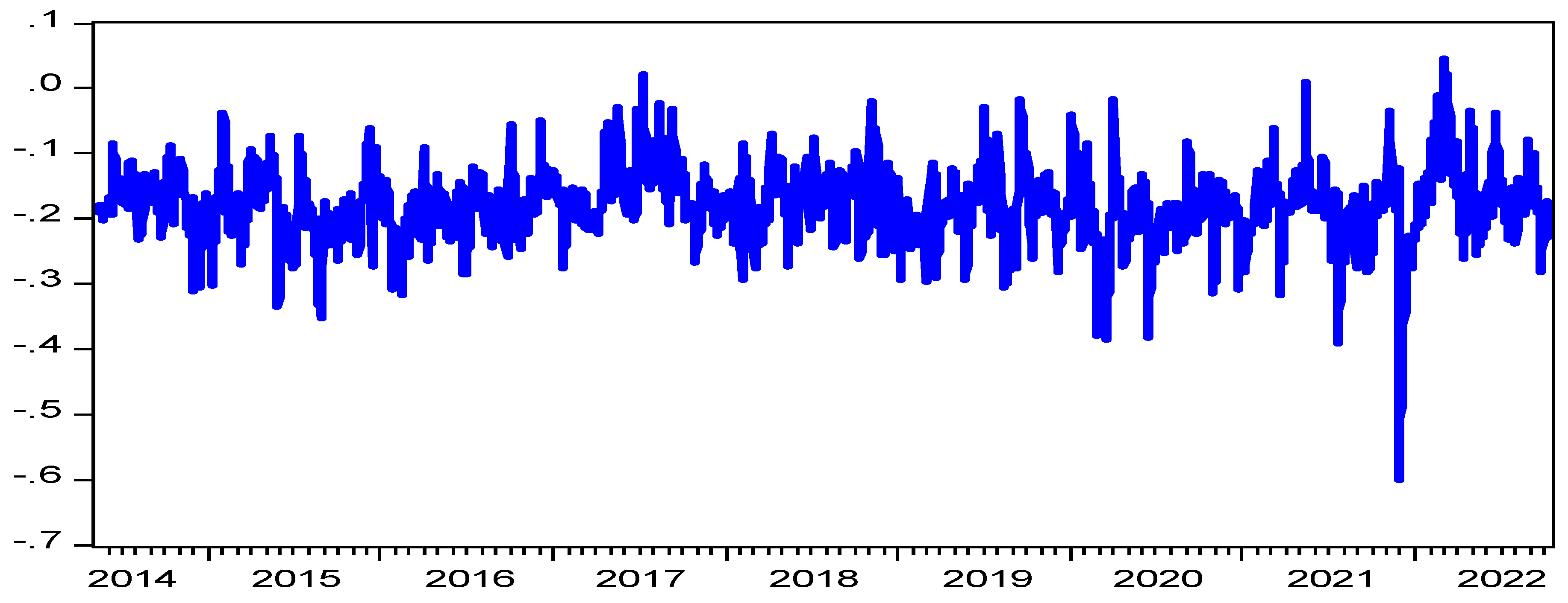
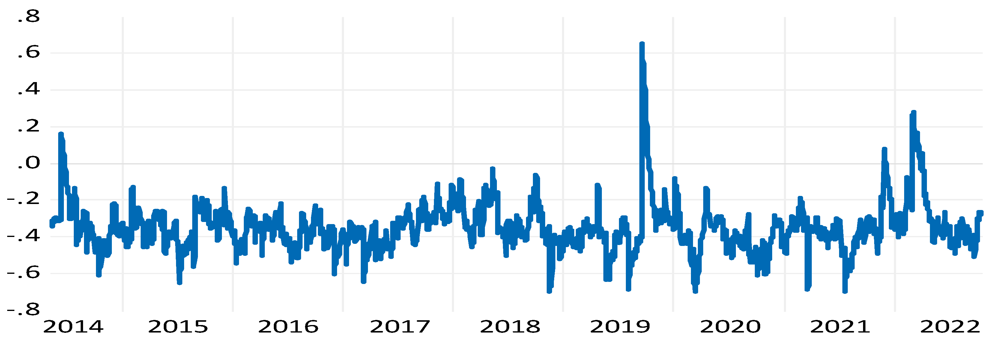
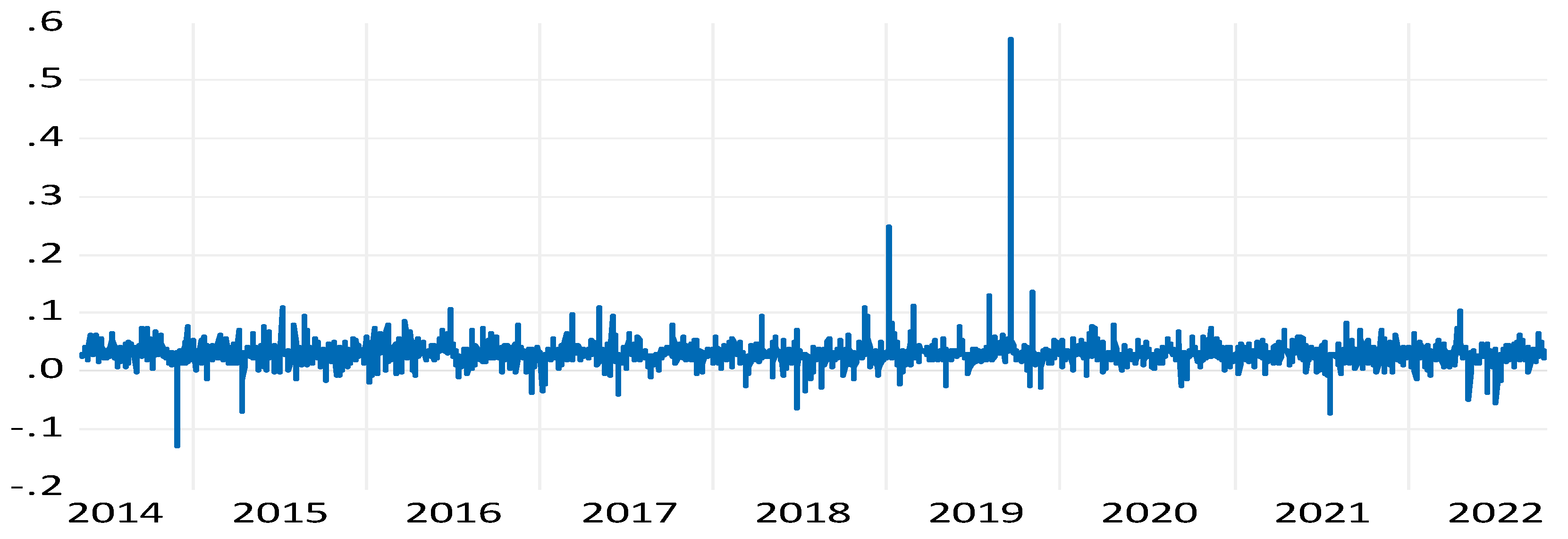
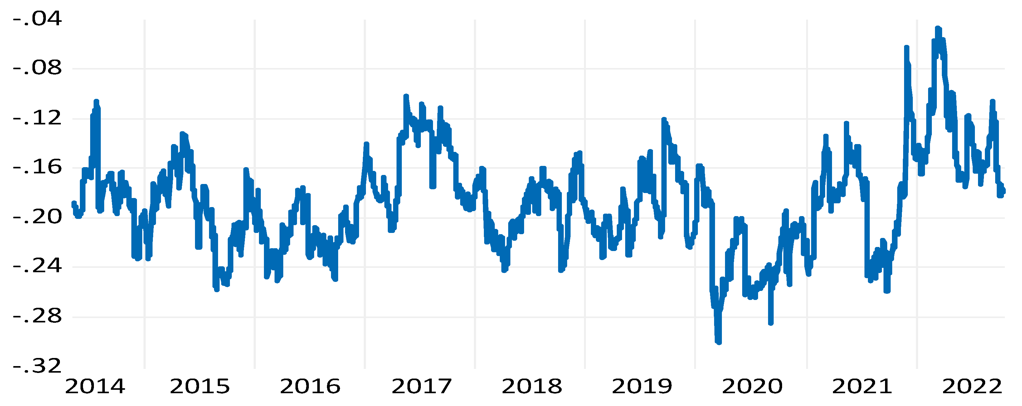
The dynamic conditional correlation between the BRENT return and the various uncertainty indices is plotted in Figure 1, Figure 2, Figure 3, Figure 4 and Figure 5, respectively. The dynamic connectedness for the BRENT oil-RBEI peer (Figure 1) is positive, indicating that there is a positive correlation between the oil market and the commodity uncertainty index. The BRENT oil-ROVX peer graph (Figure 2), on the other hand, shows that the ROVX shock has a considerable, negative effect on the BRENT return. This provides evidence that crude oil risk innovations affect adversely the oil market and vice versa.

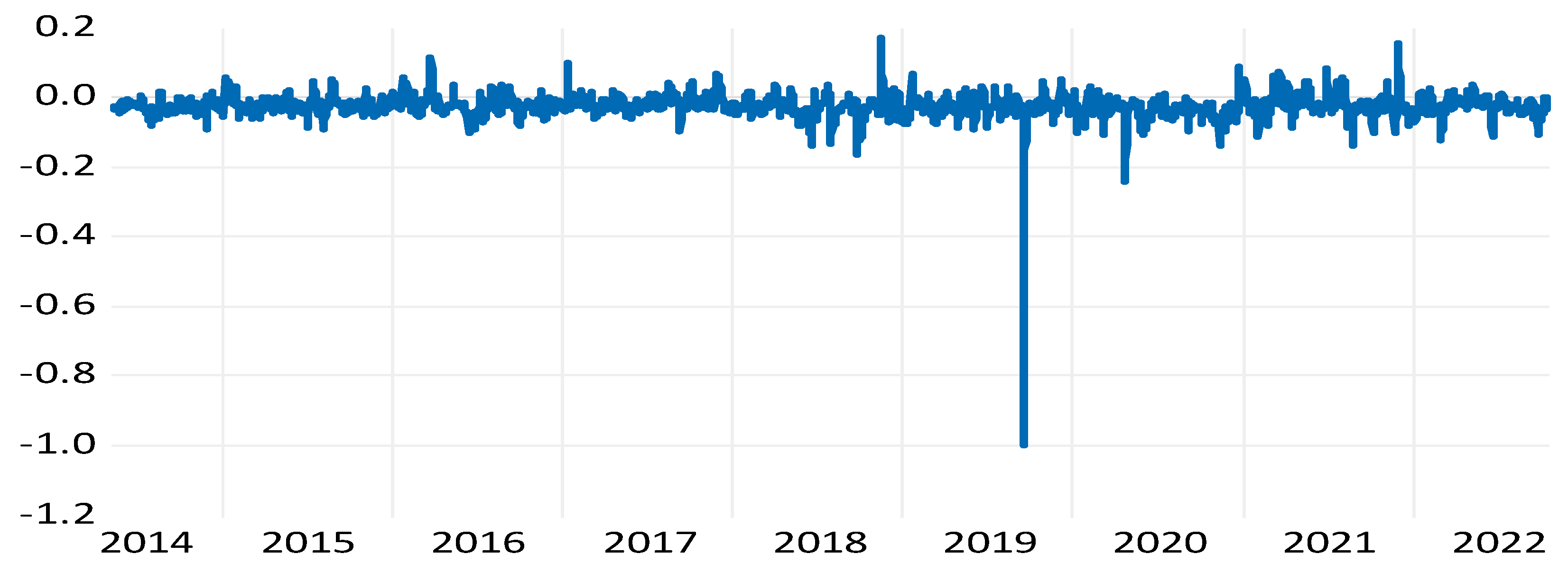
However, Figure 3 and Figure 4 display different findings. We find that the dynamic conditional correlation between REPU and RGPR shocks and the BRENT return is practically insignificant as the DCC values are around zero.

For the BRENT return and the RVIX index (Figure 5), we observe that the shock to RVIX has a significantly negative link to the BRENT return. This provides evidence that crude oil risk innovations affect adversely the oil market and vice versa.

4.2.2. Spectral Analysis

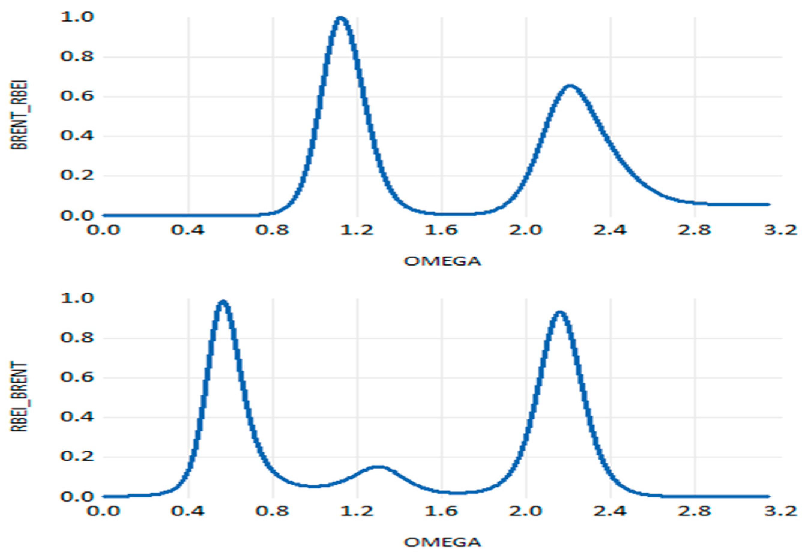
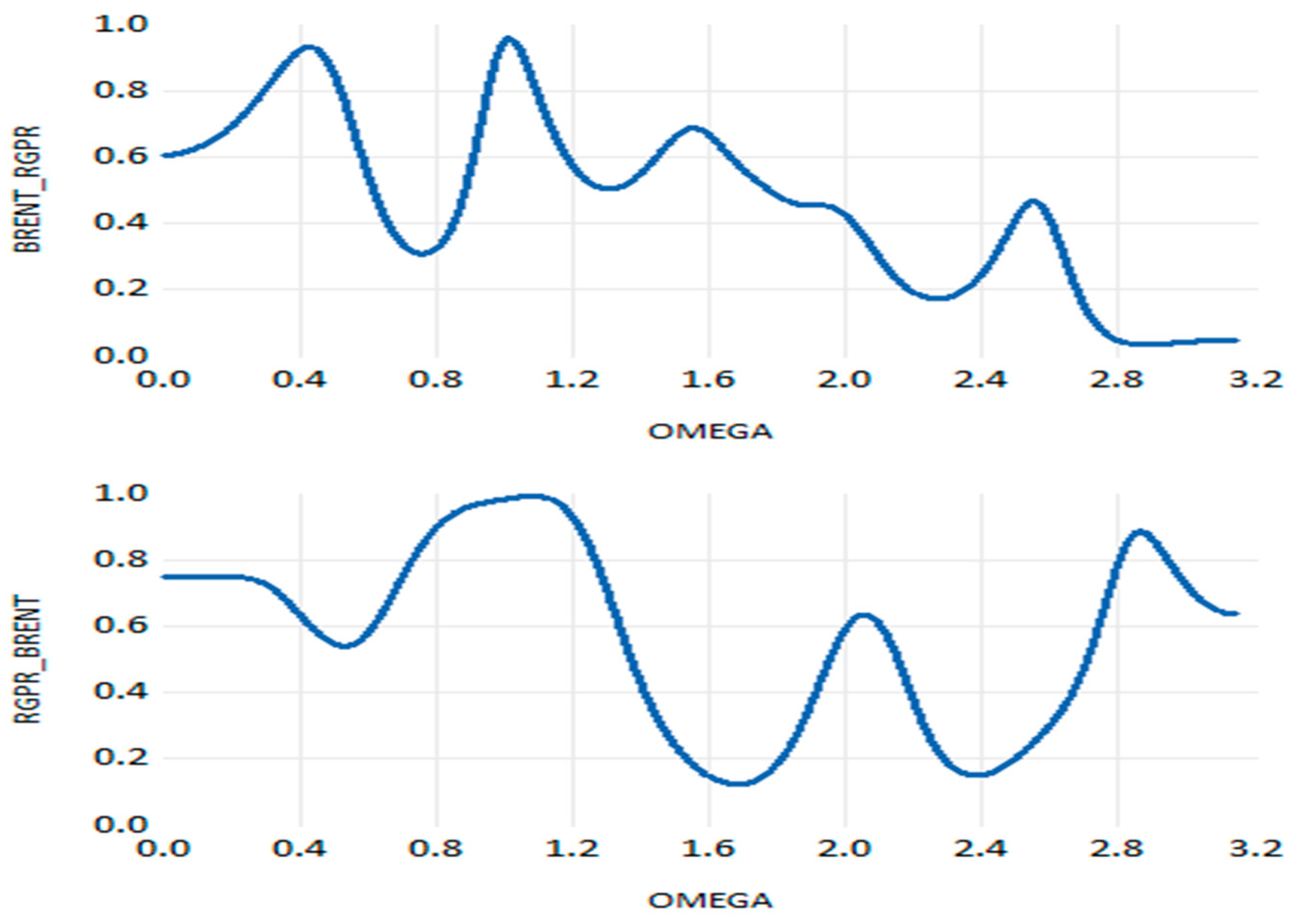
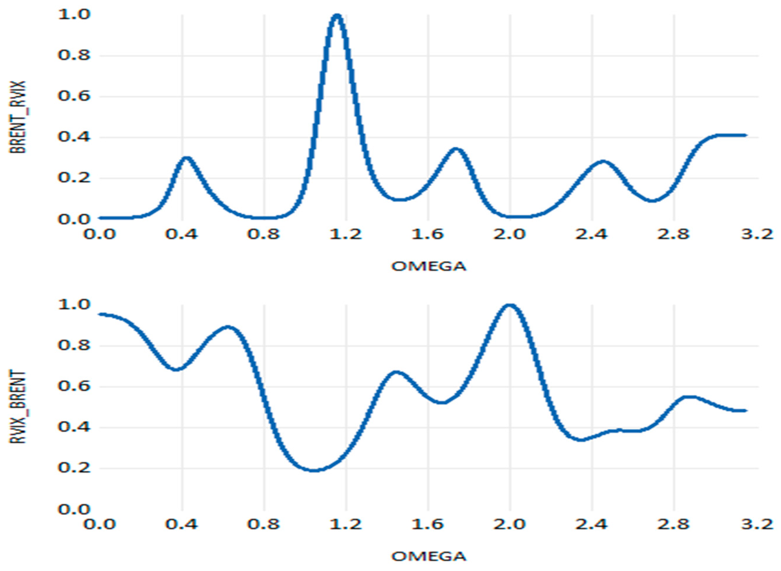
The Granger causality test is then applied in the frequency domain to examine the direction of the causal influence at every point in the frequency distribution between the return on crude oil and the different measures of uncertainty. This is completed after applying the DCC-GARCH approach to analyze the dynamic conditional correlation between the variables. Figure 6, Figure 7, Figure 8, Figure 9 and Figure 10 provide a plot of the results calculated using this approach. Every figure has a probability y-axis and an abscissa axis representing frequency OMEGA(ω), which is equal to 2Π/length of the cycle (T). Ref. [43] has determined that the medium period is seen to be two to five years, the long term as five years or longer, and the short term as less than two years.

Figure 6 illustrates the causality from the crude oil return to the RBEI index and vice versa. Empirical results show that the causality from RBEI index to crude oil return is significant throughout a range of frequencies (ω) from 0.00203 to 0.909 and from 1.38 to 1.94. This indicates a persistent dynamic spillover causality in the long run. A short-run effect of the RBEI index on crude oil return is also detected. We find that the effect is significant over the frequencies (ω) that span from 2.65 to 3.14. This means that a significant spillover effect from the short- to long-term horizon goes from commodity market uncertainty to the oil market. This is consistent with the findings from the DCC-GARCH method estimates. Thus, the contagion effect from the commodity market to the oil market is shown. For the effect of the oil market on the commodity market uncertainty, the same pattern is observed. The effect is significant in the long-term throughout a range of frequencies (ω) from 0.00203 to 0.385, from 0.838 to 1.17, and from 1.41 to 1.90 and in the short run throughout a range of frequencies (ω) from 2.40 to 3.14. This finding supports the economic intuition provided by [44] that commodity and energy markets have grown interwoven as a result of financialization, which may amplify the effects of direct and indirect risks across markets. This interconnection can be due to factors such as the similarity of market players, the correlation of global economic events, or even consumption trends. It also shows that movements in one market can trigger immediate or nearly immediate reactions in the other market, suggesting a significant interdependence between the two. On the financial side, this indicates that when it comes to portfolio management with diversified assets, traders must play an important part in energy-commodities assets management. On the economic side, our results are in line with the findings of [45], which illustrated that the analysis of factors influencing the commodity market and vice versa is important to understand inflation and macroeconomic issues.

Given that there is a significant causal relationship between the BRENT return and the RBEI index, the findings presented in Figure 7 show that the causal relationship between the BRENT return and the REPU is not significant for all frequencies in either direction, except in the spillover effect of the BRENT return on the REPU where the impact is significant in the long run for the frequencies ranging from 0.00203 to 0.389. This does not support the DCC-GARCH model’s conclusions that there is no spillover impact between the oil market and shocks to the US policy economy.

On the contrary, Figure 8 provides evidence of no significant causality from BRENT’s return to RGPR. However, this figure plots that the content information of the geopolitical risk index has a significant short-run impact on the crude oil return over a range of frequencies (from ω = 2.73 to ω = 3.14). This contradicts the DCC-GARCH findings that there is no effect of geopolitical tensions on the crude oil market. This indicates that political insecurity and geopolitical considerations have a huge influence on oil prices, and the impact is first indirect in the short run, but when events impacting energy supplies unfold, the impact in the long run becomes direct, resulting in supply scarcity and high prices.

In Figure 9, we also present the estimation results of the Granger causality test conducted for the BRENT oil return-ROVX peer. Empirically, there is also clear evidence of the significant spectral causality between the uncertainty of crude oil and the return on Brent oil. However, we discover that the causality from the ROVX index to crude oil return is significant throughout a range of frequencies (ω) from 0.64 to 0.74, from 1.07 to 2.16, and from 2.42 to 3.14. This indicates a persistent dynamic spillover causality in the long run as well as in the short run. This suggests that an ongoing oil uncertainty shock is the significant determinant of the return on crude oil.

As well, we see a considerable financial market spillover effect in the co-movement of the BRENT oil return and RVIX (Figure 10). Empirically, it was demonstrated that there was considerable spectral causality from the RVIX to BRENT oil return throughout a range of frequencies (ω) from 0.00203 to 0.318, from 0.57 to 0.97, from 1.43 to 1.49, from 1.87 to 2.25, and from 2.65 to 2.72. This suggests that dynamic spillover causation persists in the long run as well as in the short term. The significant spillover effect of uncertainty from the financial market to the crude oil market can be considered in line with the foundation of Modern Portfolio Theory (MPT). This theory indicates that achieving an efficient allocation of capital in a balanced portfolio composed of various assets such as stocks and crude oil necessitates understanding the interconnection between crude oil and financial markets and the contagion effect between them to balance potential returns and risks. On the other hand, the uncertainty brought on by the US financial market cannot be impacted by changes in BRENT oil return. There is no discernible causal link in the opposite direction, indicating that the oil market has no spectral influence on the American financial market.

5. Robustness Analysis

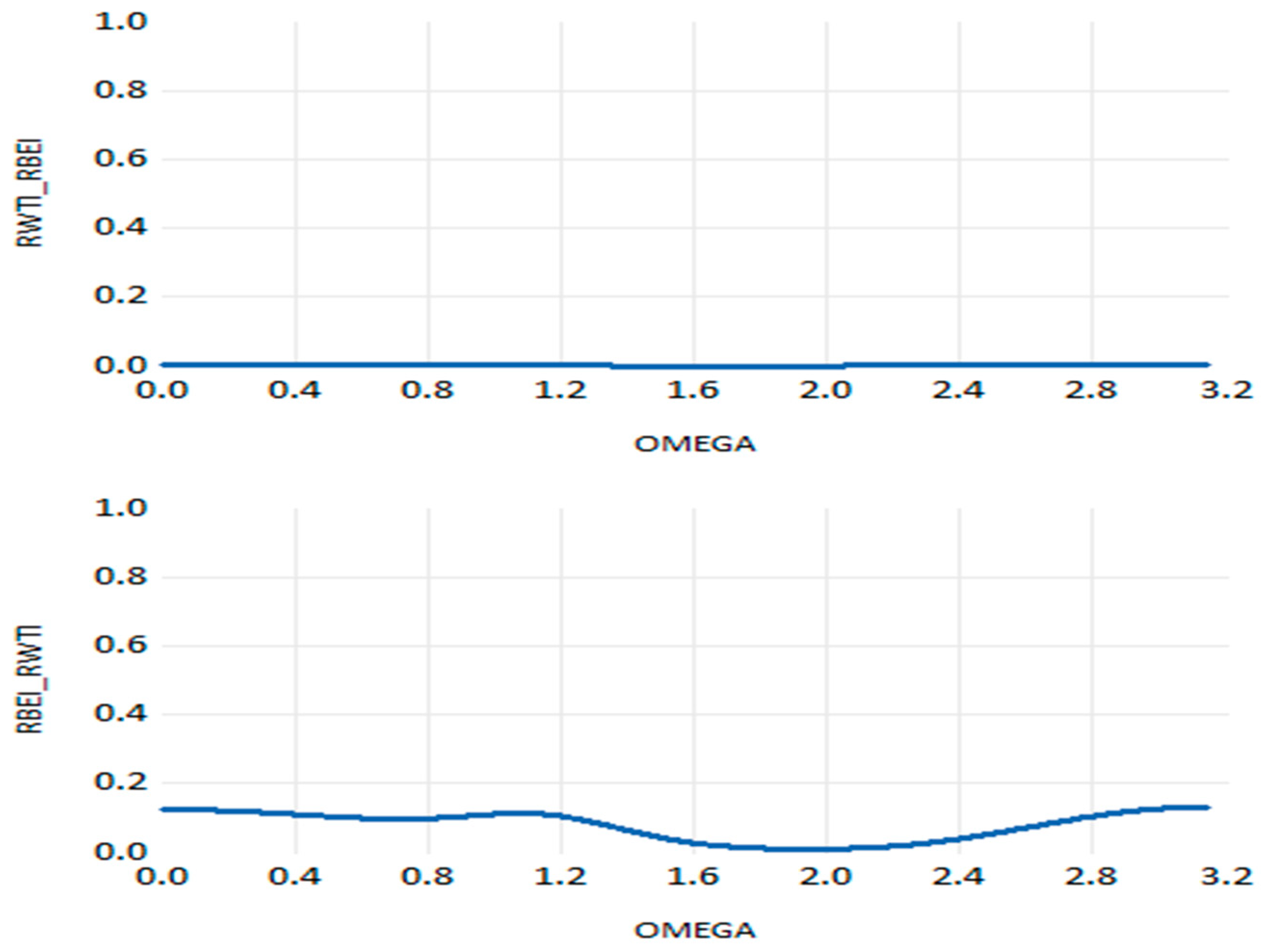
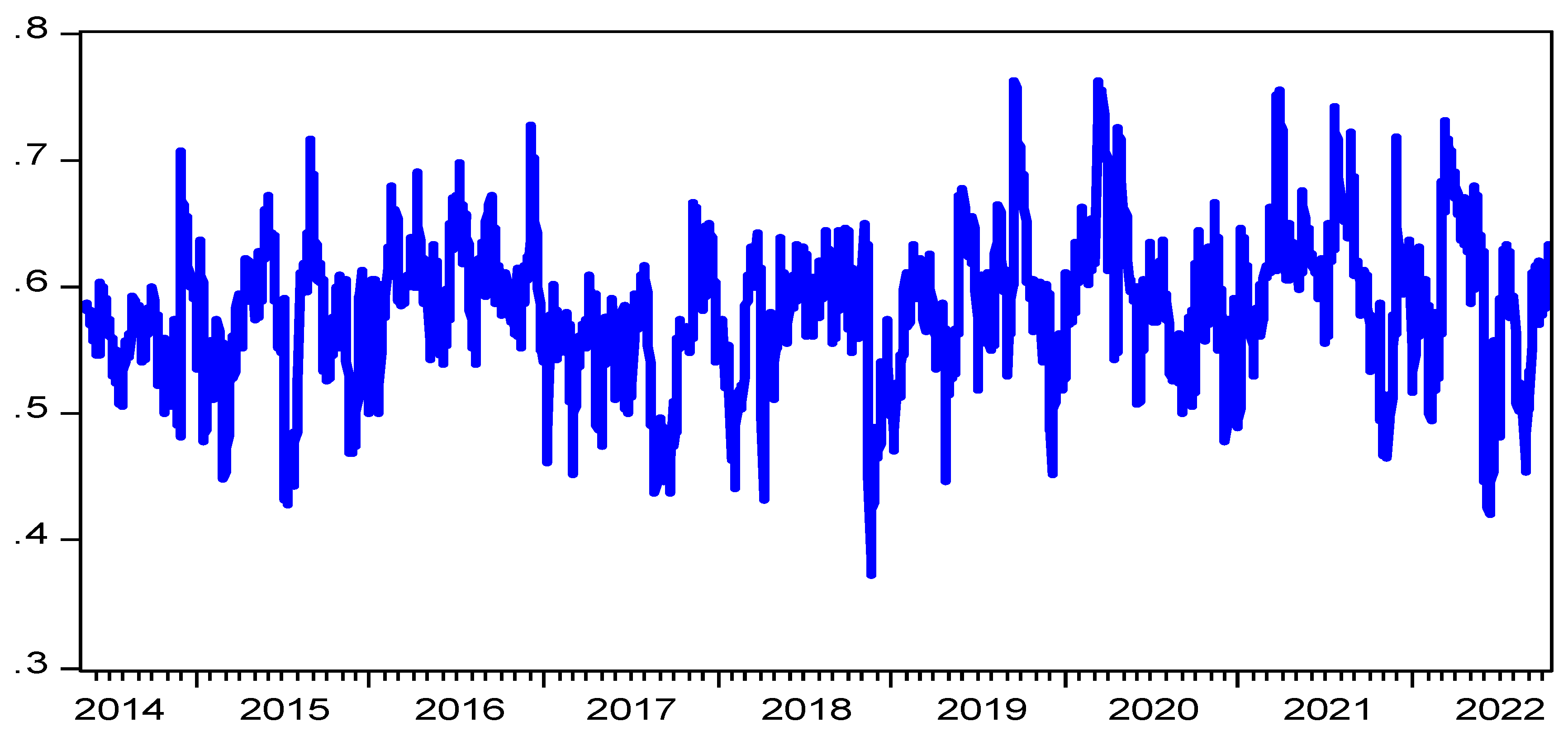
This section is allocated to assess the robustness of our main results. We apply the DCC-GARCH (1.1) model and the Granger causality test in the frequency domain to explain the WTI crude return by using the uncertainty factors. First, the results of DCC-GARCH (1.1) model estimations are plotted in Figure 11, Figure 12, Figure 13, Figure 14 and Figure 15. The results are similar to those presented in the BRENT example. More specifically, the dynamic connectedness for the WTI oil return-RWTI peer (Figure 1) is positive, demonstrating a positive link between the oil market and the commodities uncertainty index. The WTI oil return-ROVX peer graph (Figure 2), On the other hand, demonstrates that the ROVX shock has a significant, negative influence on the WTI oil return. This shows that crude oil risk innovations negatively impact the oil market and vice versa.

Figure 3 and Figure 4 show distinct results. We find that the dynamic conditional correlation between REPU and RGPR shocks and the WTI return is inconsequential since the DCC values are close to zero.

We find that the shock to the RVIX index has a strong negative relationship with the WTI return (Figure 15). This demonstrates that crude oil risk innovations negatively impact the oil market and vice versa.

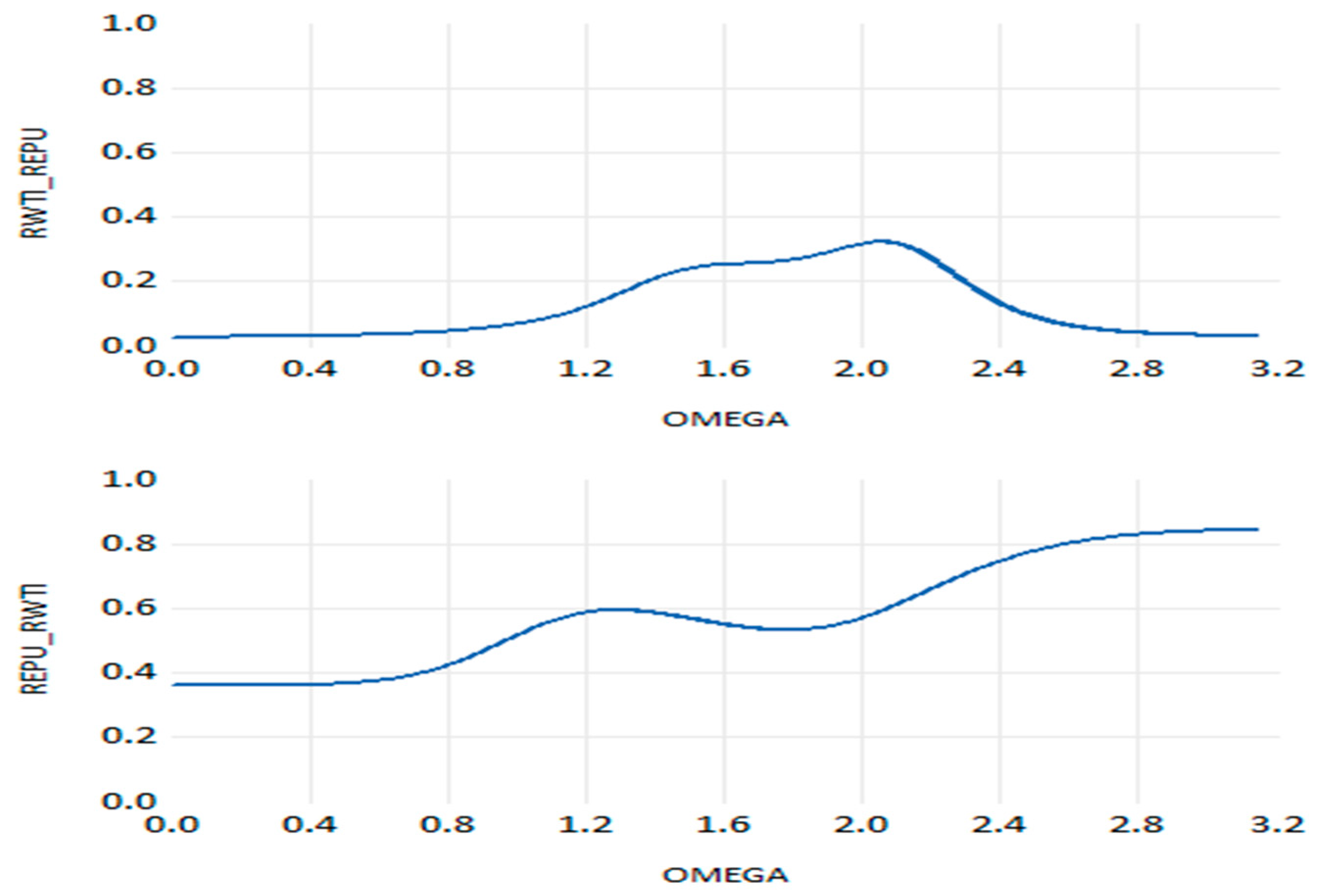
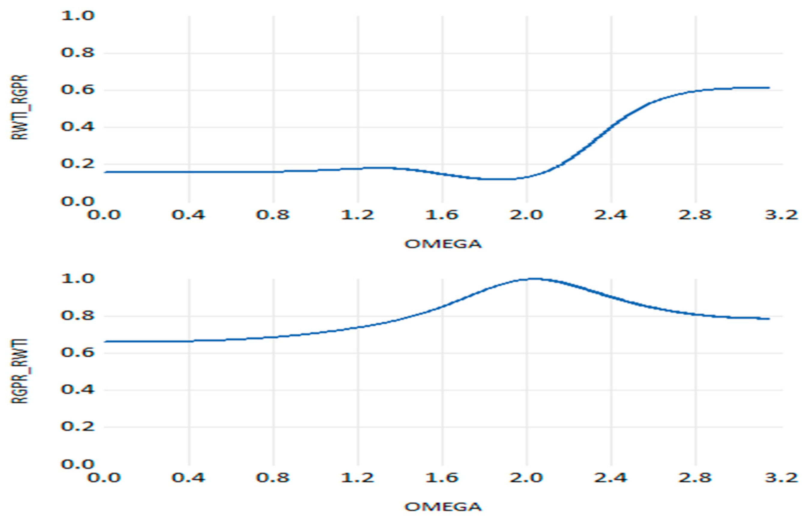
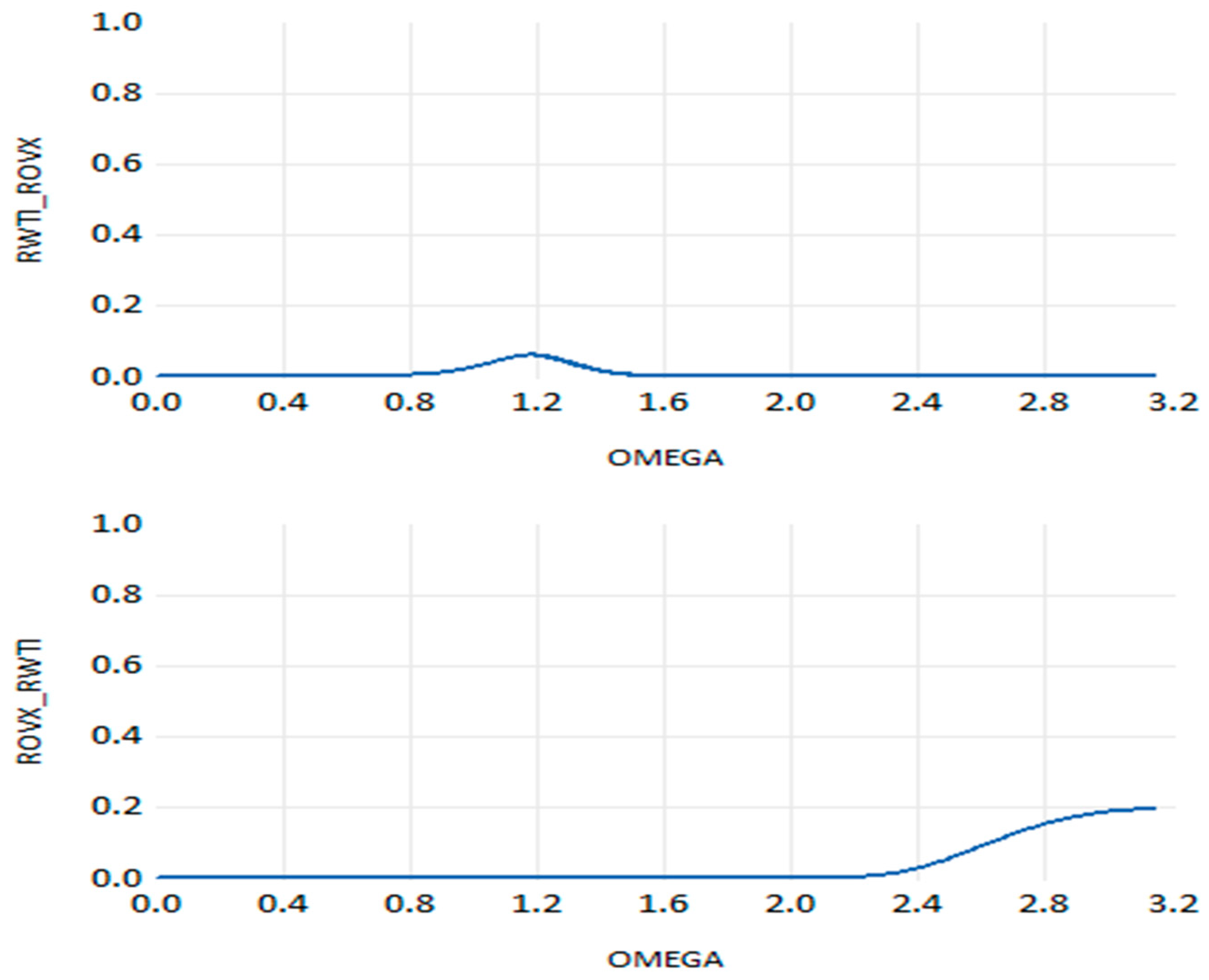
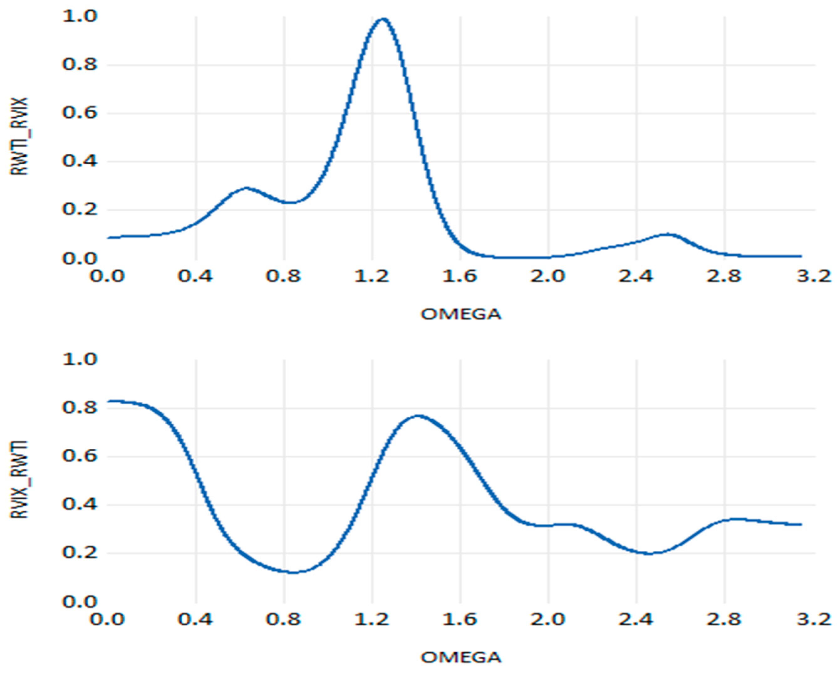
Now we consider the Granger causality test in the frequency domain to investigate the direction of the causal relationship between the WTI return on crude oil and the various metrics of uncertainty. This is completed after analyzing the dynamic conditional correlation between the variables using the DCC-GARCH technique. For the link between WTI oil return and RBEI (Figure 16), we find a significant spillover effect from uncertainty in the commodity market to the crude oil market over all different frequencies (from ω = 0.00203 to ω = 3.14). This indicates a permanent dynamic spillover causality from short to long-term horizon running from uncertainty of the commodity market to the oil market. Thus, the significant effect of uncertainty in the commodity market on the oil market is more pronounced in the WTI case than in the BRENT case. Regarding the nexus between WTI oil return and EPU (Figure 17), findings provide evidence of a significant effect from the EPU to WTI oil return over different frequencies (from ω = 0.00203 to ω = 1.13 and from ω = 2.46 to ω = 3.14). This means that the transmission of uncertainty caused by the economic policy has a short- and long-run effect on the WTI oil return. However, a non-significant effect was proven for the reverse direction. In addition to this, Figure 18 plots the interaction between WTI oil return and GPR. Non-significant causality between two variables in both directions has been detected. Concerning the nexus between WTI oil return and OVX, Figure 19 provides evidence of a significant spillover effect from uncertainty in the energy market to WTI oil return over all different frequencies (from ω = 0.00203 to ω = 3.14). In the reverse direction, the causality is significant in both the long run and short run over the frequencies that range from ω = 0.00203 to ω = 2.62. Finally, for the relationship between WTI oil return and implied volatility (RVIX), Figure 20 illustrates that there was considerable spectral causality from the RVIX to WTI oil return throughout a range of frequencies (ω) from 0.00203 to 0.24 and from 1.59 to 3.14. This suggests that dynamic spillover causation persists in the long run as well as in the short term from the financial market to the oil market.

6. Conclusions and Policy Recommendations

Given that they are so important in discussions of energy and economic issues, we concentrated in this work on the dynamic spillover effects between the crude oil market and uncertainty. Considering this, we suggested the DCC-GARCH model and the Granger causality test in the frequency domain for daily data from 2014 to 2022. The findings of the DCC-GARCH estimations demonstrated that the dynamic conditional correlations for BRENT oil-RBEI, BRENT oil-ROVX, and BRENT oil-RVIX are significant, which suggests that conditional correlations have significantly changed over time. These results support Celik’s outcomes (2012). These findings imply that a contagion effect may be responsible for the highest correlation between the oil market and other sources of uncertainty. The results also indicate that in contrast to sources with low volatility persistence, sources with high volatility persistence have more substantial interactions with the oil market. Furthermore, the findings indicate that there is no obvious long-term dynamic association between crude returns and risk innovations brought about by the US political economy and US geopolitical events. For the EPU, these results contradict the findings of [25] that all EPU indexes can have a considerable short- and long-term impact on West Texas Intermediate returns when using a DCC-GARCH model. Regarding the geopolitical risk index, our findings are different from [34], which show that geopolitical risk is found to have a positive association with oil returns and a negative correlation with stock returns, according to the results of the DCC model. Overall, the significance of most of the many relationships was observed using the DCC-GARCH test. Identifying the direction of the causal relationship between variables involves applying the Granger causality test in the frequency domain.

The findings of the spectral causality test supported the existence of persistent causality that connects the uncertainty of commodity markets to the oil markets and vice versa. We also stressed that Brent oil returns will always be driven by crude oil uncertainty. In agreement with [46], which showed that higher uncertainty indices have a positive impact on crude oil returns only at specific periods, we also demonstrate how uncertainty from the US financial market spills over to the oil market and helps to explain crude oil returns. Empirically, we discover that the implied volatility risk’s uncertainty has a significant impact on the returns of oil in the short run as well as in the long run. In addition, we identify a long-run effect of the US political economy on the crude oil return. However, a short-run effect of geopolitical risk events on the crude oil return is detected. Consequently, the following intriguing findings were made: First, the oil market is significantly impacted in the short, medium, and long terms by shocks in the commodity, energy, and financial markets. This suggests that these shocks have a lasting effect on oil return. In contrast to US geopolitical events and US circumstances for economic policy, we see more frequent spillovers of uncertainty from US commodities, energy, and financial markets to international oil markets. This suggests that market uncertainty-related shocks are more likely to affect the oil market than shocks caused by other sources.

Our findings have several policy implications. First, it is critical that investors and regulators correctly pinpoint the variables influencing oil returns. According to our research, uncertainty in the US commodity, energy, and financial markets is a significant factor in explaining crude oil returns. Because of this, it is crucial that energy policymakers continually enhance their control and attention to these diverse sources of uncertainty through mitigation and hedging strategies. As a result, experienced traders like energy ETFs are becoming more confident. Due to the resulting rise in risk perception, optimal asset allocation and increased investment in energy-risky assets like oil futures are generated. But if decision-makers do not keep an eye on and rein in the uncertainty that is spreading from the financial and commodity markets, it will make novice investors more anxious about the future of their wealth and portfolios. Therefore, rather than investing in oil futures, these investors should put their money into real assets like the stock of energy companies. For example, on 20 April 2020, oil prices, specifically American crude oil, fell below zero for the first time in history, reaching a negative price estimated at $37.63 per barrel, which surprised many investors and the general public alike and increased investor uncertainty. In the oil industry, one of the causes of the crisis was that inexperienced traders held the May 2020 contracts until the end of the last session before the settlement date, failing to get rid of them and sell them to oil refineries that refrained from buying due to the market’s double shock. In the end, they are compelled to accept the raw resources. However, because the vast majority of May contract holders were traders with no need for oil as a commodity, most of them rushed to get rid of the contract at any cost to avoid having to receive the oil themselves, and they were willing to pay money to whoever wanted to buy that contract from them. Many of these traders not only lost their money but may have borrowed to avoid the contract at any cost. This example demonstrates that investors must first understand that as speculators, they will be playing in a limited time frame and that by the time the settlement date arrives, they must have sold the contract unless they have a desire to receive oil, but they must pay attention. One contract calls for the delivery of 1000 barrels of crude oil, which must be stored somewhere. Furthermore, defensive equities are a good way for investors to balance and lower risk when uncertainties are higher. Second, the spread of persistent uncertainty from the energy, commodities, and financial markets to the oil market is a risky sign of volatility in the oil market, pushing investors to reconsider injecting liquidity into environmentally friendly energy companies. This study had some valuable findings, but it also had several flaws. First, this study focuses solely on the transmission of uncertainty between the oil market and other sources of uncertainty, neglecting the possibility of spillovers in the risk domain that go beyond volatility. Future studies should focus on tail risk spillovers. Exploring extreme risk spillovers within oil markets presents an intriguing and essential avenue for future research [47,48]. Understanding how extreme events propagate through these markets, causing sudden and profound impacts on interconnected sectors, economies, and global financial systems, is critical. Investigating the mechanisms and dynamics of extreme risk transmission from oil markets to other financial markets during periods of heightened volatility or geopolitical tensions can shed light on systemic vulnerabilities and contagion pathways. Furthermore, delving into the implications of such extreme spillovers on asset pricing, risk management strategies, and policy frameworks could offer invaluable insights for market participants, regulators, and policymakers seeking to enhance market resilience and mitigate the impact of extreme events in the future. Second, the research topic was not addressed from the aspect of forecasting. Utilizing artificial intelligence techniques like particle swarm optimization (PSO) to predict the return of crude oil can help enhance the trial findings of this study in the future.

References

1. Hamilton, J.D. What is an oil shock? J. Econom. 2003, 113, 363–398. [Google Scholar] [CrossRef]
2. Ftiti, Z.; Tissaoui, K.; Boubaker, S. On the relationship between oil and gas markets: A new forecasting framework based on a machine learning approach. Ann. Oper. Res. 2022, 313, 915–943. [Google Scholar] [CrossRef]
3. Tissaoui, K.; Zaghdoudi, T.; Hakimi, A.; Nsaibi, M. Do Gas Price and Uncertainty Indices Forecast Crude Oil Prices? Fresh Evidence Through XGBoost Modeling. Comput. Econ. 2022, 16, 1–25. [Google Scholar] [CrossRef]
4. Charles, A.; Darné, A. Volatility persistence in crude oil markets. Energy Policy 2014, 65, 729–742. [Google Scholar] [CrossRef]
5. Gatfaoui, H. Linking the gas and oil markets with the stock market: Investigating the US relationship. Energy Econ. 2016, 53, 5–16. [Google Scholar] [CrossRef]
6. Wu, B.; Wang, L.; Lv, S.X.; Zeng, Y.R. Effective crude oil price forecasting using new text-based and big-data-driven model. Measurement 2021, 168, 108468. [Google Scholar] [CrossRef]
7. Dutta, A.; Bouri, E.; Saeed, T. News-based equity market uncertainty and crude oil volatility. Energy 2021, 222, 119930. [Google Scholar] [CrossRef]
8. Wei, Y.; Liu, J.; Lai, X.; Hu, Y. Which determinant is the most informative in forecasting crude oil market volatility: Fundamental, speculation, or uncertainty? Energy Econ. 2017, 68, 141–150. [Google Scholar] [CrossRef]
9. Ma, R.; Zhou, C.; Cai, H.; Deng, C. The forecasting power of EPU for crude oil return volatility. Energy Rep. 2019, 5, 866–873. [Google Scholar] [CrossRef]
10. Nonejad, N. Forecasting crude oil price volatility out-of-sample using news-based geopolitical risk index: What forms of nonlinearity help improve forecast accuracy the most? Financ. Res. Lett. 2022, 46, 102310. [Google Scholar] [CrossRef]
11. Celık, S. The more contagion effect on emerging markets: The evidence of DCC-GARCH model. Econ. Model. 2012, 29, 1946–1959. [Google Scholar] [CrossRef]
12. Yousaf, I.; Ali, S. The COVID-19 outbreak and high frequency information transmission between major cryptocurrencies: Evidence from the VAR-DCC-GARCH approach. Borsa Istanb. Rev. 2020, 20, S1–S10. [Google Scholar] [CrossRef]
13. Yıldırım, D.Ç.; Esen, Ö.; Ertuğrul, H.M. Impact of the COVID-19 pandemic on return and risk transmission between oil and precious metals: Evidence from DCC-GARCH model. Resour. Policy 2022, 79, 102939. [Google Scholar] [CrossRef] [PubMed]
14. Breitung, J.; Candelon, B. Testing for short-and long-run causality: A frequency-domain approach. J. Econom. 2006, 132, 363–378. [Google Scholar] [CrossRef]
15. Cheng, S.; Liu, W.; Jiang, Q.; Cao, Y. Multi–Scale Risk Connectedness Between Economic Policy Uncertainty of China and Global Oil Prices in Time–Frequency Domains. Comput. Econ. 2023, 61, 1593–1616. [Google Scholar] [CrossRef]
16. Bagheri, E.; Ebrahimi, S.B.; Mohammadi, A.; Miri, M.; Bekiros, S. The dynamic volatility connectedness structure of energy futures and global financial markets: Evidence from a novel time–frequency domain approach. Comput. Econ. 2022, 59, 1087–1111. [Google Scholar] [CrossRef]
17. Bozoklu, S.; Yilanci, V. Energy consumption and economic growth for selected OECD countries: Further evidence from the Granger causality test in the frequency domain. Energy Policy 2013, 63, 877–881. [Google Scholar] [CrossRef]
18. Pérez-Montiel, J.A.; Manera, C. Is autonomous demand really autonomous in the United States? An asymmetric frequency-domain Granger causality approach. Metroeconomica 2022, 73, 78–92. [Google Scholar] [CrossRef]
19. Bandi, F.M.; Chaudhuri, S.E.; Lo, A.W.; Tamoni, A. Spectral factor models. J. Financ. Econ. 2021, 142, 214–238. [Google Scholar] [CrossRef]
20. Cao, Y.; Cheng, S.; Li, X. How economic policy uncertainty affects asymmetric spillovers in food and oil prices: Evidence from wavelet analysis. Resour. Policy 2023, 86, 104086. [Google Scholar] [CrossRef]
21. Zhu, H.; Chen, W.; Hau, L.; Chen, Q. Time-frequency connectedness of crude oil, economic policy uncertainty and Chinese commodity markets: Evidence from rolling window analysis. N. Am. J. Econ. Financ. 2021, 57, 101447. [Google Scholar] [CrossRef]
22. Jiang, Q.; Cheng, S.; Cao, Y.; Wang, Z. The asymmetric and multi-scale volatility correlation between global oil price and economic policy uncertainty of China. Environ. Sci. Pollut. Res. 2022, 29, 11255–11266. [Google Scholar] [CrossRef] [PubMed]
23. Chai, J.; Xing, L.M.; Zhou, X.Y.; Zhang, Z.G.; Li, J.X. Forecasting the WTI crude oil price by a hybrid-refined method. Energy Econ. 2018, 71, 114–127. [Google Scholar] [CrossRef]
24. Zhang, Y.; Ma, F.; Wang, Y. Forecasting crude oil prices with a large set of predictors: Can LASSO select powerful predictors? J. Empir. Financ. 2019, 54, 97–117. [Google Scholar] [CrossRef]
25. Zhang, Y.J.; Yan, X.X. The impact of US economic policy uncertainty on WTI crude oil returns in different time and frequency domains. Int. Rev. Econ. Financ. 2020, 69, 750–768. [Google Scholar] [CrossRef]
26. Tissaoui, K.; Zaghdoudi, T.; Hakimi, A.; Ben-Salha, O.; Ben Amor, L. Does Uncertainty Forecast Crude Oil Volatility before and during the COVID-19 Outbreak? Fresh Evidence Using Machine Learning Models. Energies 2022, 15, 5744. [Google Scholar] [CrossRef]
27. Wang, Y.; Cheng, S.; Cao, Y. How does economic policy uncertainty respond to the global oil price fluctuations? Evidence from BRICS countries. Resour. Policy 2022, 79, 103025. [Google Scholar] [CrossRef]
28. Niu, Z.; Ma, F.; Zhang, H. The role of uncertainty measures in volatility forecasting of the crude oil futures market before and during the COVID-19 pandemic. Energy Econ. 2022, 112, 106120. [Google Scholar] [CrossRef]
29. Chen, B.X.; Sun, Y.L. The impact of VIX on China’s financial market: A new perspective based on high-dimensional and time-varying methods. N. Am. J. Econ. Financ. 2022, 63, 101831. [Google Scholar] [CrossRef]
30. Benedetto, F.; Mastroeni, L.; Quaresima, G.; Vellucci, P. Does OVX affect WTI and Brent oil spot variance? Evidence from an entropy analysis. Energy Econ. 2020, 89, 104815. [Google Scholar] [CrossRef]
31. Chen, Z.; Liang, C.; Umar, M. Is investor sentiment stronger than VIX and uncertainty indices in predicting energy volatility? Resour. Policy 2021, 74, 102391. [Google Scholar] [CrossRef]
32. Lu, X.; Ma, F.; Wang, J.; Wang, J. Examining the predictive information of CBOE OVX on China’s oil futures volatility: Evidence from MS-MIDAS models. Energy 2020, 212, 118743. [Google Scholar] [CrossRef] [PubMed]
33. Qian, L.; Zeng, Q.; Li, T. Geopolitical risk and oil price volatility: Evidence from Markov-switching model. Int. Rev. Econ. Financ. 2022, 81, 29–38. [Google Scholar] [CrossRef]
34. Smales, L.A. Geopolitical risk and volatility spillovers in oil and stock markets. Q. Rev. Econ. Financ. 2021, 80, 358–366. [Google Scholar] [CrossRef]
35. Engle, R. Dynamic conditional correlation: A simple class of multivariate generalized autoregressive conditional heteroskedasticity models. J. Bus. Econ. Stat. 2002, 20, 339–350. [Google Scholar] [CrossRef]
36. Lean, H.H.; Teng, K.T. Integration of world leaders and emerging powers into the Malaysian stock market: A DCC-MGARCH approach. Econ. Model. 2013, 32, 333–342. [Google Scholar] [CrossRef]
37. Tissaoui, K.; Azibi, J. International implied volatility risk indexes and Saudi stock return-volatility predictabilities. N. Am. J. Econ. Financ. 2019, 47, 65–84. [Google Scholar] [CrossRef]
38. Geweke, J.F. Measures of conditional linear dependence and feedback between time series. J. Am. Stat. Assoc. 1984, 79, 907–915. [Google Scholar] [CrossRef]
39. Gomez-Gonzalez, J.E.; Villamizar-Villegas, M.; Zarate, H.M.; Amador, J.S.; Gaitan-Maldonado, C. Credit and business cycles: Causal effects in the frequency domain. Ens. Sobre Política Económica 2015, 33, 176–189. [Google Scholar] [CrossRef]
40. Tissaoui, K. Forecasting implied volatility risk indexes: International evidence using Hammerstein-ARX approach. Int. Rev. Financ. Anal. 2019, 64, 232–249. [Google Scholar] [CrossRef]
41. Tzeremes, P. Oil volatility index and Chinese stock markets during financial crisis: A time-varying perspective. J. Chin. Econ. Foreign Trade Stud. 2021, 14, 187–201. [Google Scholar] [CrossRef]
42. Lovcha, Y.; Perez-Laborda, A. Long-memory and volatility spillovers across petroleum futures. Energy 2022, 243, 122950. [Google Scholar] [CrossRef]
43. Prats, M.A.; Sandoval, B. Does stock market capitalization cause GDP? A causality study for Central and Eastern European countries. Economics 2020, 14, 20200017. [Google Scholar] [CrossRef]
44. Khan, K.; Su, C.W.; Koseoglu, S.D. Who are the influencers in the commodity markets during COVID-19? Resour. Policy 2022, 78, 102854. [Google Scholar] [CrossRef]
45. Ben Ameur, H.; Boubaker, S.; Ftiti, Z.; Louhichi, W.; Tissaoui, K. Forecasting commodity prices: Empirical evidence using deep learning tools. Ann. Oper. Res. 2023, 1–19. [Google Scholar]
46. Aloui, R.; Gupta, R.; Miller, S.M. Uncertainty and crude oil returns. Energy Econ. 2016, 55, 92–100. [Google Scholar] [CrossRef]
47. Liu, Z.; Shi, X.; Zhai, P.; Wu, S.; Ding, Z.; Zhou, Y. Tail risk connectedness in the oil-stock nexus: Evidence from a novel quantile spillover approach. Resour. Policy 2021, 74, 102381. [Google Scholar] [CrossRef]
48. Qian, L.; Jiang, Y.; Long, H. Extreme risk spillovers between China and major international stock markets. Mod. Financ. 2023, 1, 30–34. [Google Scholar] [CrossRef]
Figure 1. DCC between BRENT and RBEI.
Energies 17 00340 g001
Figure 2. DCC between BRENT and ROVX.
Energies 17 00340 g002
Figure 3. DCC between BRENT and REPU.
Energies 17 00340 g003
Figure 4. DCC between BRENT and RGPR.
Energies 17 00340 g004
Figure 5. DCC between BRENT and RVIX.
Energies 17 00340 g005
Figure 6. Spectrum analysis: Granger causality between BRENT and RBEI.
Energies 17 00340 g006
Figure 7. Spectrum analysis: Granger causality between BRENT and REPU.
Energies 17 00340 g007
Figure 8. Spectrum analysis: Granger causality between BRENT and RGPR.
Energies 17 00340 g008
Figure 9. Spectrum analysis: Granger causality between BRENT and ROVX.
Energies 17 00340 g009
Figure 10. Spectrum analysis: Granger causality between BRENT and RVIX.
Energies 17 00340 g010
Figure 11. DCC between WTI and RBEI.
Energies 17 00340 g011
Figure 12. DCC between WTI and ROVX.
Energies 17 00340 g012
Figure 13. DCC between WTI and REPU.
Energies 17 00340 g013
Figure 14. DCC between WTI and RGPR.
Energies 17 00340 g014
Figure 15. DCC between WTI and RVIX.
Energies 17 00340 g015
Figure 16. Spectrum analysis: Granger causality between WTI and RBEI.
Energies 17 00340 g016
Figure 17. Spectrum analysis: Granger causality between WTI and REPU.
Energies 17 00340 g017
Figure 18. Spectrum analysis: Granger causality between WTI and RGPR.
Energies 17 00340 g018
Figure 19. Spectrum analysis: Granger causality between WTI and ROVX.
Energies 17 00340 g019
Figure 20. Spectrum analysis: Granger causality between WTI and RVIX.
Energies 17 00340 g020