Article

Estimation of Differential Capacity in Lithium-Ion Batteries Using Machine Learning Approaches

Sustainable Energy Systems Research Group, Department of Energy and Process Engineering, Faculty of Engineering, NTNU, NO-7491 Trondheim, Norway
*
Author to whom correspondence should be addressed.
Energies 2024, 17(19), 4954; https://doi.org/10.3390/en17194954
Submission received: 30 August 2024 / Revised: 18 September 2024 / Accepted: 2 October 2024 / Published: 3 October 2024
(This article belongs to the Section D: Energy Storage and Application)

Abstract

:
Comprehending the electrochemical condition of a lithium-ion battery (LiB) is essential for guaranteeing its safe and effective operation. This insight is increasingly obtained through characterization tests such as a differential capacity analysis, a characterization test well suited for the electric transportation sector due to its dependency on the available voltage and current (E–I) data. However, a drawback of this technique is its time dependency, as it requires extensive time due to the need to conduct it at low charge rates, typically around C/20. This work seeks to forecast characterization data utilizing 1C cycle data at increased temperatures, thereby reducing the time required for testing. To achieve this, three neural network architectures were utilized as the following: a recurrent neural network (RNN), feed forward neural network (FNN), and long short-term memory neural network (LSTM). The LSTM demonstrated superior performance with evaluation scores of the mean squared error (MSE) of 0.49 and mean absolute error (MAE) of 4.38, compared to the FNN (MSE: 1.25, MAE: 7.37) and the RNN (MSE: 0.89, MAE: 6.05) in predicting differential capacity analysis, with all models completing their computations within a time range of 49 to 299 ms. The methodology utilized here offers a straightforward way of predicting LiB degradation modes without relying on polynomial fits or physics-based models. This work highlights the feasibility of forecasting differential capacity profiles using 1C data at various elevated temperatures. In conclusion, neural networks, particularly an LSTM, can effectively provide insights into electrochemical conditions based on 1C cycling data.

1. Introduction

Lithium-ion batteries (LiBs) are crucial for the transition toward green energy, predominantly in the transportation sector, where LiBs have become essential for the development of battery electric vehicles (BEVs) [1,2]. Since the predominant expenses and life cycle emissions of LiBs are linked to battery production, extending the lifespan of batteries can significantly reduce their overall emissions [3,4].
Over time, the capacity of LiBs gradually diminishes due to various mechanical and chemical degradation mechanisms [5,6,7]. Battery aging is heavily influenced by operating conditions, with extreme temperatures and rapid reaction rates accelerating the degradation process [8,9]. This aging process reduces the power output and energy storage capacity of LiBs [6]. Therefore, understanding the internal state of a battery is crucial for ensuring proper operation and preventing misuse and safety incidents [10]. Given the complexity of LiBs as electrochemical energy storage devices, direct assessment is not feasible, making accurate estimations essential for optimal Battery Management System (BMS) functionality [11,12].
Numerous characterization techniques exist for lithium-ion batteries, each possessing distinct advantages and disadvantages. The choice of technique depends on the intended output and the available equipment [13]. Nevertheless, pseudo-OCV and differential capacity analysis are more advantageous than electrochemical impedance spectroscopy [14] and are suitable for use in BEVs as they only require the available voltage and current, that is, the E–I data. Furthermore, analytical methods have been developed to improve the accessibility of differential capacity analysis [15]. However, a common issue with traditional characterization techniques is their time-consuming nature, with a full differential capacity test taking 40 h to run [16]. Machine learning (ML) can be employed to precisely forecast attributes such as the State of Charge (SoC) and State of Health (SoH) [11,17,18]. Recently, the field of battery technology has entered a new era emphasizing data-intensive and computational approaches, known as the fourth paradigm of science [19,20]. ML has become a potent instrument in battery characterization, providing a viable remedy for the drawbacks of conventional methods [21].
Although ML has shown promising results in overcoming time constraints, most studies have focused on predicting model-based labels like SoH, SoC, and impedance, or on smaller data sequences [11]. Nevertheless, intricately analyzed characterization data, such the dQ/dV profiles from differential capacity analysis, can offer significant understanding into the principles underlying the degradation as well as the degradation itself [13,22,23]. The ohmic resistance increase (ORI), loss of lithium inventory (LLI), and loss of active materials (LAM) from the electrodes’ are some of these mechanisms [5,6,7].
Typically, the charging phase of a differential capacity analysis takes 20 h to complete at a charge rate of C/20 [16] and is conducted at a standardized ambient temperature, as temperature and heat produced from charge rates affect the thermodynamic state of an LiB [24]. Predicting differential capacity analysis results using data collected in one hour (1C) could reduce the testing time by 95%. If effective, this strategy could increase the accessibility of precise state predictions, highlighting the importance of LiBs in green transition.
This study aims to utilize ML methodology to predict standardized differential capacity analysis results for the charge phase using 1C charge data at an elevated temperature (defined as 25 °C and above) instead of relying on the slow C/20 characterization. Moreover, this study intends to reduce the time required for differential capacity analysis by avoiding the requirement for C/20 cycling data and leveraging ML to allow the use of 1C data for differential capacity analysis. By using 1C data, we attempted to provide processed characterization data in time-sensitive situations under the ambient temperatures different from 25 °C. The focus was on gradual capacity loss due to degradation modes, excluding power fade. For the ML models, we assumed the availability of characterization data from the LiB’s Beginning of Life. While not all cycled cells undergo a complete differential capacity study, noteworthy results and broad trends were highlighted in relation to the projections of the machine learning model.
In the following sections, we present the methodology and the results of our study. Section 2 describes the materials and methods used in battery cycling, the machine learning methodology, and the machine learning approaches used in this article. Section 3 covers a selection of the differential capacity results, followed by the results from the neural networks used in differential capacity prediction. Section 4 covers the discussion of the findings followed by the overall conclusions in Section 5.

2. Materials and Methods

2.1. Battery Cycling and Data Collection

2.1.1. Battery Production

The LiB cells used in this investigation had a nominal capacity of 0.2 Ah and were designed as pouch cells. Each cell featured a wound structure, comprising an NMC111 cathode and an artificial graphite anode. The anode was connected to a copper current collector, and the cathode was connected to an aluminum current collector. Both collectors had double coatings. The cells were sourced from LiFUN and were delivered without an electrolyte. Prior to formation cycling and aging cycling, the cells were filled with an electrolyte (1 M LiPF6 in a 50:50 EC:DMC solvent) inside a glovebox to shield it from unfavorable environments. Following assembly, the batteries were cycled using a battery cycling system (Arbin Instruments, College Station, TX, USA; MitsPro 8.0) within temperature chambers (VWR®, UK; INCU-Line 250R).

2.1.2. Battery Testing

A program to optimize the value of the gathered data was created in order to use the testing program’s data for machine learning across a range of temperatures. External limits including the time constraints, requirement for dependable data, and availability of testing channels greatly impacted the design of this testing program. The findings of Waldmann et al. (2014) [8] indicated that the primary degradation mechanisms differed above and below 25 °C. Therefore, the selected temperature range for this study included 25 °C, 35 °C, and 45 °C. To obtain a dataset for each temperature condition, a sample of six cells was analyzed at 25 °C, five cells at 35 °C, and six cells at 45 °C.

2.1.3. Battery Formation Cycling

The formation process for the LiB cells commenced immediately after assembly and removal from the glovebox. The cells were then placed in their designated channels within the temperature chambers. The formation program, based on the methodology of An et al. (2017) [25], utilized a rapid formation process with characteristics similar to traditional slow formation programs. This formation process was conducted at 25 °C.

2.1.4. Battery Aging Cycling

Following the formation cycling, the cells were subjected to an aging and characterization schedule. The cycling was conducted between the upper and lower voltage limits of 4.2 V and 3 V, as specified by the cell manufacturer. Given that the state of an LiB is highly influenced by temperature, all cells were characterized at a consistent temperature of 25 °C for practical and performance reasons. The cycling for aging the LiBs was performed at the designated temperatures.
As the aging and characterization stages changed, the experiments were stopped and the chamber temperature was modified. The temperature change process took time, and once the chosen temperature was attained, the cells were allowed to stabilize for two hours to ensure they reached the chamber temperature.

2.1.5. Battery Characterization

At the Beginning of Life (BoL) and after every 50 cycles, a characterization test was performed at 25 °C. An investigation of differential capacity was performed using a C/20 discharge and a C/20 charge. Prior to discharge, the cell was charged using a constant current and the constant voltage (CCCV) method (CC: 1C, CV: 4.2V) with an exit condition of current ≤ C/20 to ensure a full charge before testing. Following CCCV charging, all capacities were reset and the batteries rested for five minutes. The differential capacity analysis was performed for the charge phase between the lower and upper voltage limits, with data logged every 60 s. A 5 min rest period was included between discharge and charge phases. Following the conclusion of the investigation of differential capacity, all capacities were reset.
Since differential capacity is the change in charge over the change in voltage, data processing was necessary. The differential capacity characterization approach gives raw data. The MATLAB function “smoothdata”, which smooths entries using a moving window without fitting a polynomial to the full dataset, was used to process the noisy data points produced by differential capacity, employing the quadratic regression method “loess” on the voltage data (either charge or discharge) with the filter window set to 170. Based on a deterioration map with three characteristics of interest—FOI 1, FOI 2, and FOI 3—an analysis of the curves was conducted using the methodology outlined by Dubarry et al. [22].

2.2. Machine Learning Methodology

2.2.1. Task and Objective

The goal of using ML to forecast characterization data was to perhaps lessen the frequency of fresh characterizations that were required. The goal that was selected was an “immediate cycling data approach”, in which the target values were characterization data and the input was data from constant current (CC) charging at 1C. The target data were expressed as processed characterization data, consisting of differential capacity profiles, specifically the dQ/dV plots obtained during each characterization. This immediate cycling data approach was implemented using three ML architectures: the FNN, RNN, and LSTM networks. The FNN was selected for its ease of implementation, while the RNN and LSTM were chosen due to their similar input–output structures to the FNN, with the added advantage of accounting for memory effects. Regression was the model’s allocated task.

2.2.2. Feature Engineering

The data acquired for the ML program underwent extensive modification and processing to meet the model’s requirements. Temperature and step indexes noted as the cycle number were used directly without modification. To maintain consistent input data dimensions throughout the ML process, the voltage was standardized to a constant range of 3.4 to 3.9 V, split into 50 equally spaced increments. This range was chosen because it comprised the most significant features of the differential capacity analysis, which aimed to enhance the model performance and simplify the data structure. Linear interpolation was used to extract the data at each step.
Cycling data were collected from a 1C rate charge succeeding each characterization. From 3.6 to 4.1 V, 50 equally spaced steps were used to standardize the input data. At the second charge after characterization, measurements were gathered to make sure the cells met the specified temperatures during cycling.
The target was defined as the differential capacity profiles at each characterization, where the differential capacity profiles were calculated as detailed in Section 2.1.5. For the target values, they were defined as 50 equally spaced points of the profiles in the range of 3.4 V to 3.9 V found through linear interpolation. The general structure of a neural network is depicted in Figure 1.

2.2.3. Model

All models were implemented using Python 3.12 (64-bit) within the PyCharm Integrated Development Environment (IDE). Using the keras.RandomSearch and keras.HyperModel classes from the Keras library, the random search technique was used to establish the architecture of each model through hyperparametric tweaking. Every model was given its own inputs and labels, and for the recurrent models, k-fold cross-validation was used to stop state transfers between cells. A validation split of 0.2 was used for the FNN as the lack of memory effect made cell separation superfluous.
The evaluation data were kept for evaluating the completed models and were not used in the hyperparametric tweaking procedure. The number of layers, number of nodes per layer, activation functions, learning rate (represented by α), and layer type were all changed as parameters. For the random search, no random seed was specified. Table 1 provides specifics about the search space for these criteria.
The random search configuration for hyperparametric tuning was meticulously designed to enhance model performance. The key details were the following:
  • validation loss minimization as the objective;
  • 500 trials;
  • 2 executions per trial;
  • models validated every 10 iterations;
  • Adam optimizer;
  • Huber loss function.
Specific restrictions were imposed on the random search process. For the recurrent models, the initial two layers were set as recurrent. The first layer had “return sequence = True” to output the entire sequence instead of just the last value, while the second layer had “return sequence = False”. In addition, the output layer had a linear activation function and the same number of nodes as the target sequence. We also imposed the optimizer and loss function for the hyperparametric search and the subsequent model design. The Adam optimizer was chosen as it is robust and combines a gradient at the step alongside the second moment, allowing for adaptive step sizes based on the gradient’s magnitude at each iteration [26]. We chose the Huber loss as it is robust due to the combination of the mean squared error (MSE) for small errors and the mean absolute error (MAE) for large errors providing a balance between stability and sensitivity [27].
Following the random search, careful consideration was given to selecting the model architecture from the top performers. The choice was made based on standards intended to guarantee the robustness and generalizability of the model. Architectures that had notable declines in layer size followed by increases in layer size, or that had inconsistent activation functions in buried layers, were not included. This approach aimed to eradicate models that, notwithstanding high performance, showed signs of overfitting to the training data, which could result in poor performance on unseen data.
To train and validate the model, the below procedures were taken as the following:
  • K-fold validation:
    • 14 folds;
    • Data from one set fold definition;
    • Validation set used one time.
  • Training and evaluation:
    • After early stopping, best weights returned;
    • 10 epochs patience;
    • Adam optimizer;
    • Huber loss function.
To ensure the reproducibility of the results in the model training, two measures were implemented. Firstly, a random seed of 42 was set for the “Random”, “Numpy”, and “Tensorflow” libraries. Secondly, the oneDNN optimization in “Tensorflow” was inactivated, as it had the potential to influence computational behavior.

2.2.4. Evaluation

The performance metrics for each model were determined to be the mean absolute error (MAE) and mean squared error (MSE). The performance of a model was evaluated in two ways: first, by computing and averaging the overall performance metric for all sequences combined, and second, by analyzing the performance metrics for each arrangement independently and presenting the findings separately. Assuming the availability of Beginning of Life (BoL) characterization data, the final evaluation ignored the initial sequence prediction.
Since recurrent models rely on memory effects, separate cell datasets were not integrated. As a result, three cells with varying temperatures were used to individually assess the final models. To guarantee equity and consistency, the FNN was assessed in a similar way. To keep things uniform, all three approaches used the same three cells. The average of the three assessment scores that were derived from these cells is the final evaluation score that is shown in this article.

2.3. Machine Learning Approaches

The network topologies chosen for this article’s processed characterization data prediction are described in this section. The specific designs used for differential capacity profile sequence prediction are described in depth in each topic. In order for the models in this article to function and provide a baseline for future predictions, it was assumed that the initial characterization data were available. This assumption was predicated on the availability of such data for all commercial cells. Now that the model was exposed to the data it is supposed to forecast, the predictions and assessment of the initial characterization labels for all techniques were ignored.
The architecture for a model was determined through hyperparametric tuning within the previously defined search space. Subsequently, models were assessed using three distinct assessment sets. The subsequent sections detail the final architectures utilized, along with an overview of the data flow. The data flow within this section was intentionally simplified to facilitate reproducibility.

2.3.1. Feed Forward Neural Network

This methodology entails predicting labels using only immediate cycling data from 1C charging, along with the cycle number and temperature. Furthermore, each step incorporates the first characterization data as a baseline. The selected architectures for predicting differential capacity profiles are detailed in Table 2.

2.3.2. Recurrent Neural Network

This method predicts labels using immediate cycling data from 1C charging, along with the cycle number and ambient cycling temperature. To capture temporal dependencies, SimpleRNN layers are implemented, with the first layer having the return sequence set to “True” and the second layer having the return sequence set to “False”. Table 3 provides specifics on the architectures used to forecast differential capacity profiles.

2.3.3. Long Short-Term Memory Neural Network

This method predicts labels using immediate cycling data from 1C charging, along with the cycle number and temperature during cycling. To further capture temporal relationships, an LSTM layer is added. The first layer is specified as the LSTM (return sequence = True), while the second layer is configured as the LSTM (return sequence = False). Table 4 provides specifics on the architectures used to forecast differential capacity profiles.

3. Results

3.1. Differential Capacity Analysis

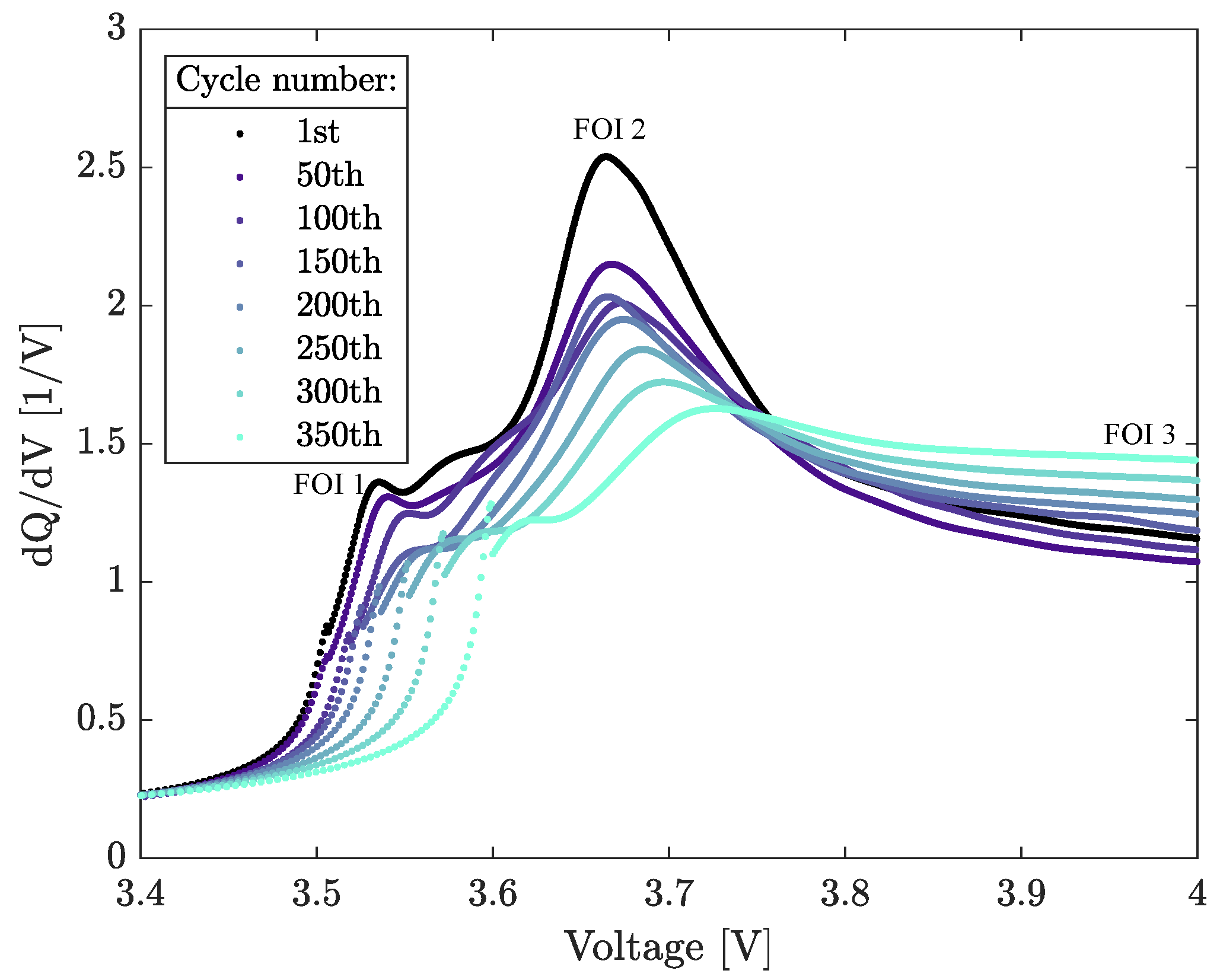
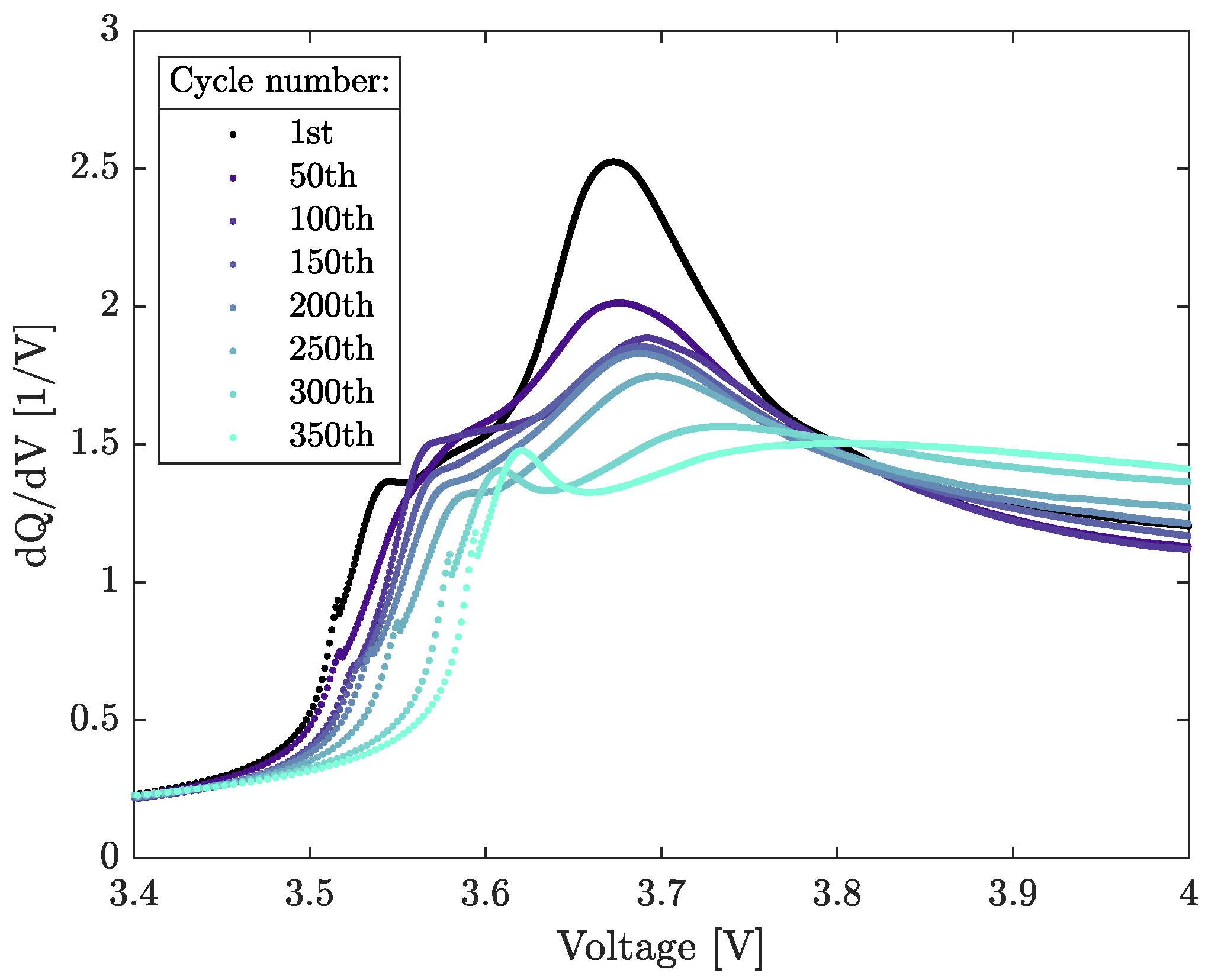
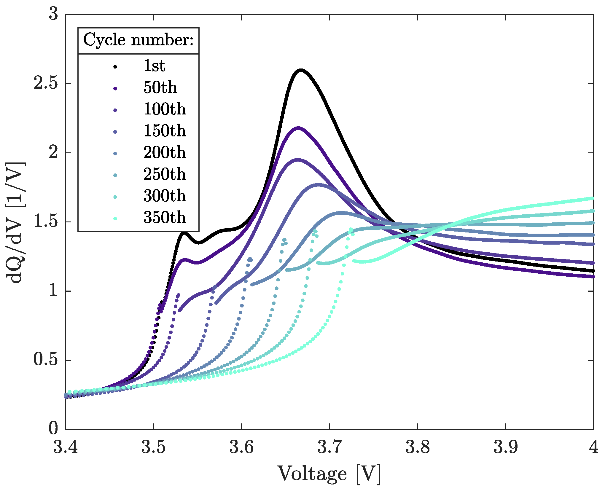
The subsequent figures illustrate the differential capacity profiles of the cells throughout their lifespan. As described by Dubarry et al., the characteristics FOI 1, FOI 2, and FOI 3 indicate the variances in these profiles [22]. Cells were cycled at 25 °C, 35 °C, and 45 °C, with a characterization cycle at 25 °C every 50th cycle.
Figure 2 depicts the differential capacity profiles of a cell cycled at 25 °C, as well as the features of interest visualized. FOI 1 shows a slight decrease toward the right in the first 100 cycles, followed by a significant drop in the peak. FOI 2 exhibits a decreasing trend and shifts toward the right. Cycling caused FOI 3 to grow gradually.
Figure 3 illustrates the cell cycled at 35 °C. FOI 1 maintained a consistent height while moving to the right. FOI 2 decreased for the initial 250 cycles. Beyond 250 cycles, it continued to decrease, though pinpointing the feature became challenging. FOI 3 exhibited a discernible increase.
Figure 4 illustrates the cell cycled at 45 °C. Following 50 cycles, FOI 1 underwent a notable rightward shift. FOI 2 exhibited a decrease and leftward shift during the initial 100 cycles, followed by further reduction near the right. FOI 2 became indistinct for cycles 300 to 350. FOI 3 experienced a significant increase.

3.2. Machine Learning

The following subsection assesses the models using data from the battery cycling experiments described earlier. Three distinct temperature representations (25 °C, 35 °C, and 45 °C) were selected for assessment. Model performance metrics are presented as the mean absolute error (MAE) and mean squared error (MSE) for each evaluation set’s average, as well as the average across all three sets, referred to as the evaluation score. The actual and projected values for each model are presented after the scores for each sequence in the evaluation sets.

3.2.1. Differential Capacity Profile Prediction Accuracy

Table 5 summarizes the performance metrics of the employed RNN, FNN, and LSTM models. The LSTM-based model demonstrated the greatest performance, achieving an MAE of 4.38 and MSE of 0.49. Following this, the RNN-based model performed second best, with an MAE of 6.05 and MSE of 0.89. Conversely, the FNN model exhibited the poorest performance, yielding an MAE of 7.37 and MSE of 1.25. Additionally, Table 5 displays the computational time ranges for the evaluation sets, run on an Acer Aspire A514-54 computer with an 11th Gen Intel® Core™ i5-1135G7 processor.
Across all models, the MAE values were relatively consistent, excluding the FNN model at 25 °C. In terms of the MSE, the 45 °C set showed the best performance across all models. Conversely, the poorest MSE score was observed in the 35 °C set for the RNN and LSTM models, and the 25 °C set for the FNN model.
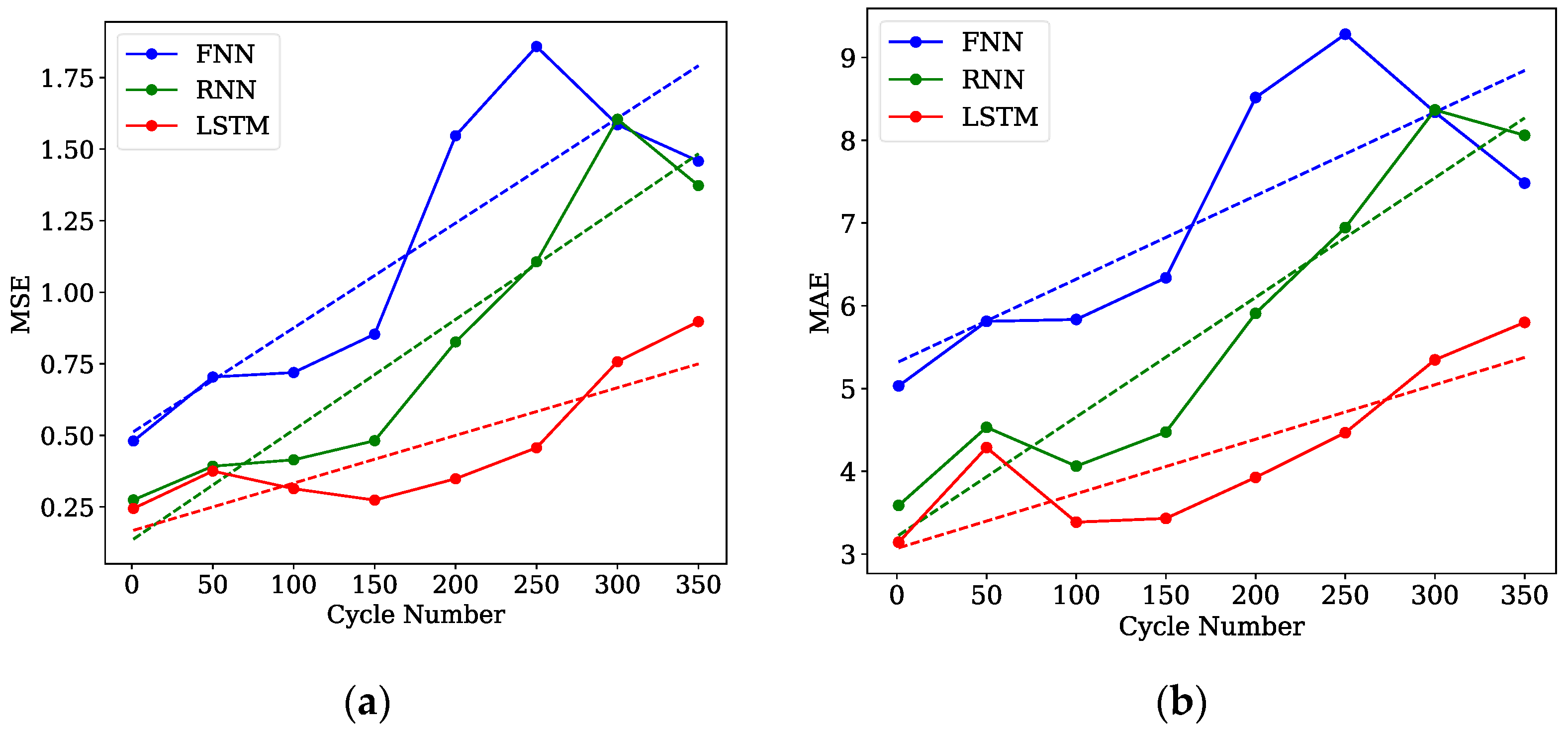
The average of the 50 labels for each sequence represents the performance metrics for each sequence in Figure 5. In all models, error increased with the cycle number. Moreover, the RNN model displayed a steeper slope in both performance metrics compared to the others. Notably, the LSTM exhibited the lowest error across all sequences and demonstrated the mildest slope for both metrics.
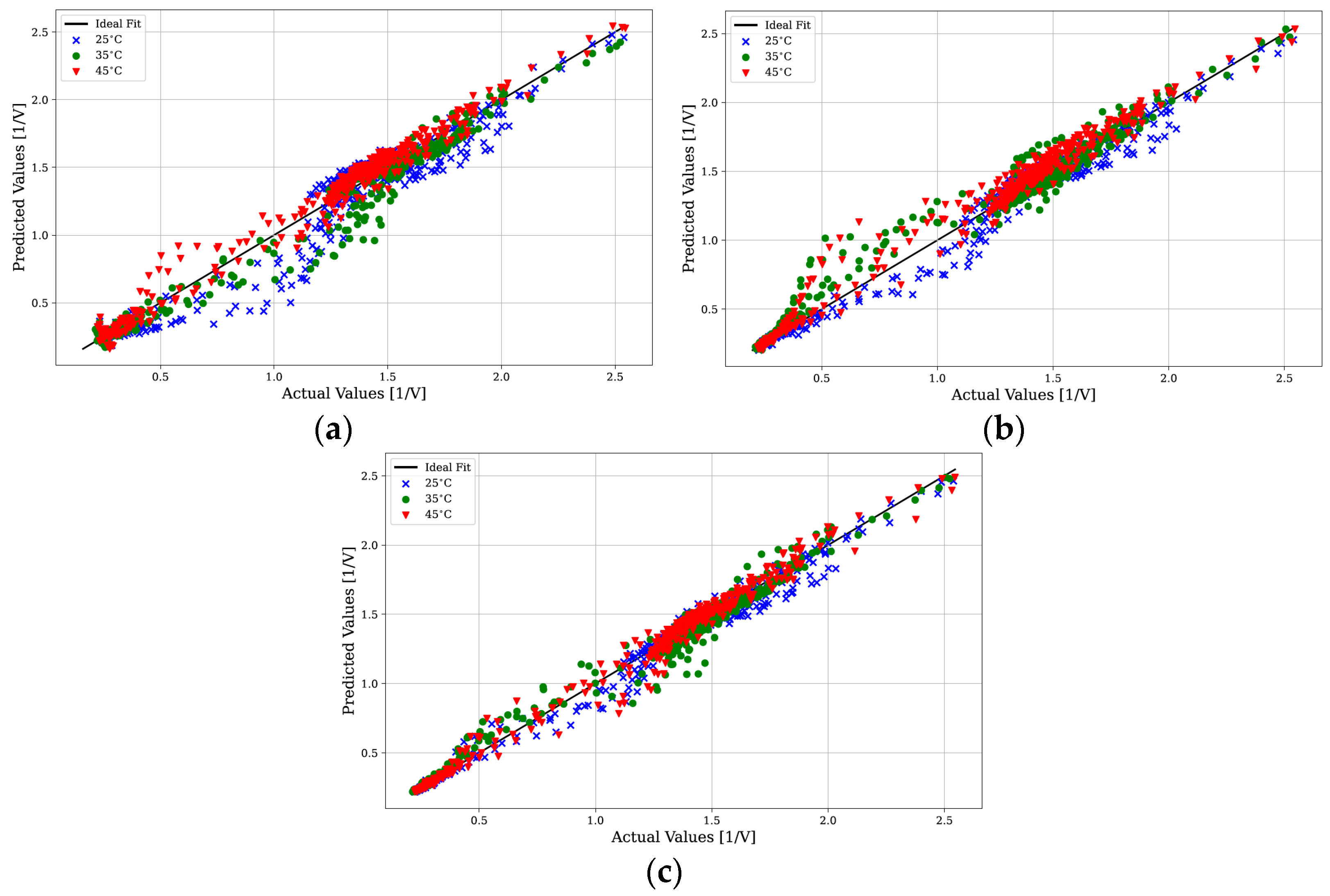
Figure 6a–c present scatter plots of actual versus predicted values for the FNN, RNN, and LSTM models, respectively. Across all models, a general pattern of deviation was observed, particularly for the 25 °C set. The most pronounced discrepancies occurred in the range of 0.5–1.25 [1/V], where both the FNN and RNN models struggled, especially for the 45 °C and 35 °C sets. The LSTM, however, showed better alignment with the ideal fit in this range.
For values below 0.5 [1/V], which corresponded to the leading edge of the differential capacity profile, the LSTM performed better than the RNN and LSTM. The FNN showed significant scatter for the lower values, while the leading edge was close to the ideal fit for the RNN and LSTM. The LSTM however stayed closer to the ideal fit as the actual values increased, while the RNN diverged quicker.
Across the range of 1 to 1.5 [1/V], all models demonstrated some degree of underprediction, most notably for the 25 °C set. The LSTM showed a slight improvement over the FNN and RNN in this range, with its predictions closer to the ideal fit. In the upper range of 1.5–2 [1/V], all models showed some values away from the ideal fit, with the LSTM still observed to be the best. However, even the LSTM began to show significant underprediction, particularly for the 25 °C set.

3.2.2. Predicted Differential Capacity Profiles

Assessing the efficacy of the neural network methodology from Figure 6 could be challenging. This section enhances the understanding of the model performance by visually comparing the predicted and actual values. The evaluation set at 45 °C was utilized for this visualization, with the model tasked to predict the differential capacity profile. Although cycle 0 data were included for reference, they were not considered in the model evaluation.
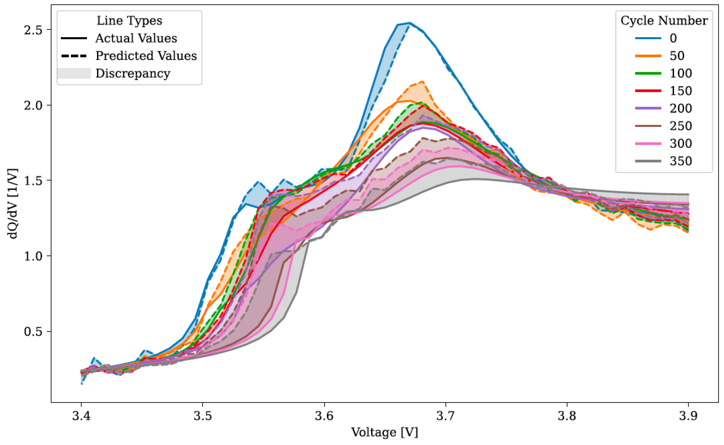
Figure 7 shows the actual results for the 45 °C evaluation set compared to the FNN model’s predictions. While the model generally captured the trend of the evaluation set, the predictions displayed noticeable noise, particularly evident in the leading edge between 3.4 and 3.5 V. This noise persisted across all sequences, making it challenging for the model to accurately foresee the ascent up to FOI 1 in later cycles. Although FOI 2’s altitude was predicted well, locating the feature was hindered by prediction noise. Evaluation of the FOI 3 shift was difficult due to the limited spread of actual values.
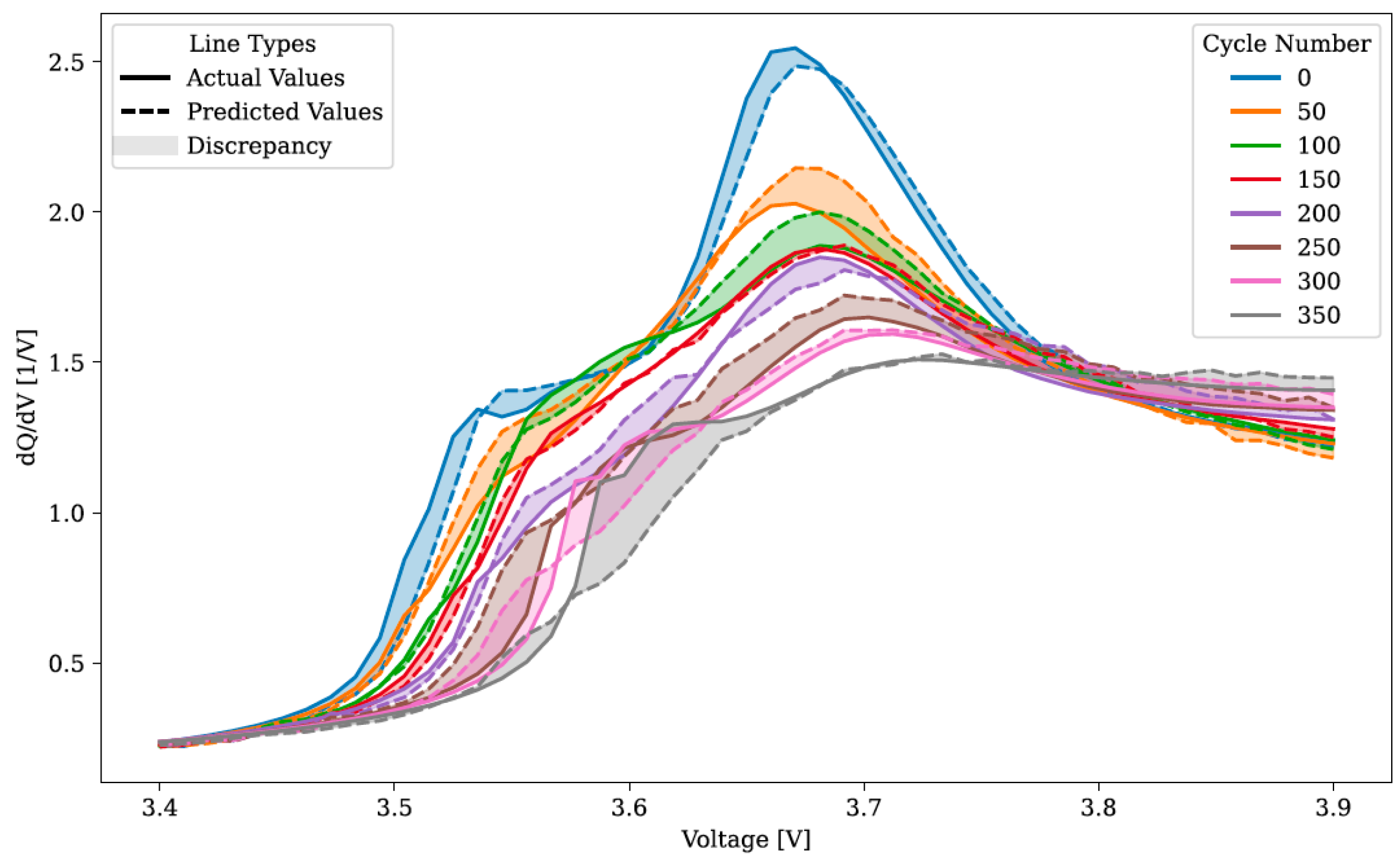
Figure 8 shows the actual values for the 45 °C evaluation set compared to the RNN model’s predictions. Like the FNN, the RNN had trouble projecting the growth prior to FOI 1. Predictions for the FOI 2 deviated significantly from actual values, worsening for larger cycle numbers. Assessing the FOI 3 was challenging due to the narrow coverage of actual values.
The LSTM model’s actual versus projected values for the 45 °C evaluation set are displayed in Figure 9. The predicted values demonstrated minimal noise within the 3.4–3.5 V range and better captured the rise prior to FOI 1 compared to the RNN and FNN models. Nonetheless, discrepancies were observed, particularly for cycles 250 to 350. Actual and expected values varied in the FOI 2, particularly at lower cycle numbers. Evaluating the FOI 3 shift was hindered by the limited spread of actual values. Notably, the LSTM model displayed smoother predictions, showing less random fluctuation in the predicted values for similar voltage levels.

4. Discussion

The performance of the final ML models was closely linked to the dataset used for training and evaluation. Figure 2, Figure 3 and Figure 4 depict the differential capacity analysis plots for all cells, revealing several trends. Notably, a significant variation in behavior, particularly the shift of FOI 1 toward higher voltages, was observed. However, accurately pinpointing the elevation of FOI 1 beyond cycle 100 remained challenging, likely due to the processing of the differential capacity analysis. To balance early and considerable cycle numbers, a filter window of 170 was applied, leading to some noise in the results, evident in the sudden jumps in most plots preceding FOI 1. Customizing the filter window for each characterization could have mitigated this issue.
Interestingly, FOI 3 was not observed during data collection. While the presence of the loss of lithium inventory (LLI) degradation mode could have pushed this feature beyond the chosen voltage window (3.4–3.9 V), it ought to have been apparent at the BoL. However, the absence of FOI 3 is a usual issue likely stemming from inhomogeneities. FOI 2, on the other hand, seems to have been the most dependable and noticeable characteristic. This underscores the limitations in predicting certain degradation modes with precision using ML models trained on this dataset.
The LSTM model beat the FNN and the RNN in predicting complicated processed characterization data, such as the differential capacity profiles. The LSTM architecture yielded an evaluation score with an MSE of 0.49 and MAE of 4.38, significantly surpassing the performance of the FNN (MSE: 1.25, MAE: 7.37) and the RNN (MSE: 0.89, MAE: 6.05). The LSTM’s greater performance could be due to its memory retention across states [28], a feature essential for modeling time-series data, as suggested by the previous literature [11,17,21]. Additionally, the low computational time of all models, with run times between 49 and 299 ms, allowed us to replace a 20 h slow characterization process at C/20 with data gathered over 1 h, effectively saving 19 h per test, while retaining the reported accuracies.
Comparing these results with prior studies underscored the significant advantage of LSTM networks in predicting time-series data crucial in battery cycle predictions. Our methodology provides a more straightforward strategy for forecasting deterioration modes than earlier research, which relied on more intricate data processing approaches like polynomial fits or the integration of physics-based modelling [29,30]. Notably, all models exhibited their largest discrepancies in the range of 0.5–1.5 [1/V], corresponding to the foremost verge before FOI 1, where horizontal shifts were primarily associated with specific degradation modes such as the LLI and ORI, as indicated by the degradation map by Dubarry et al. [22].
Over the LiB’s lifespan, the assessment ratings for all viable models rose, indicative of decreased accuracy as the cells deteriorated, consistent with the existing literature [11]. Notably, this decrease in accuracy was least pronounced for the LSTM model, underscoring its robustness. The temporal discrepancy between the baseline characterization and the degradation of the input data was probably the cause of this accuracy drop. While using a CCCV input dataset based on temporal standardization may have improved model performance, the fixed range input dataset invariably produced zero-value inputs.
Despite limitations in our methodology, our work demonstrated effectiveness in estimating differential capacity analysis under standardized conditions using immediate cycling data. Our technique permits degradation mode estimation based on 1C charge data, whereas traditional approaches have recommended low current rates (e.g., accurate at C/15, tolerable at C/4 [31]). Reducing the current rate from 1C might have improved the accuracy of the model even further. Although concerns may have arisen regarding the evaluation on cells from the same dataset as the training and validation cells [19,32], our substantial differences in differential capacity analysis results justified the validity of our evaluation.
This study established a promising framework for leveraging neural networks, particularly LSTM-based ones, to predict degradation modes under high current rates and high temperatures. Our methodology laid the groundwork for future studies to test and improve these models by offering a less complicated but probably more effective substitute for current methodologies found in the literature.

5. Conclusions

This study illustrates the viability of utilizing neural networks to predict processed characterization data gathered at C/20 using 1C charge data. It underscores the LSTM’s effectiveness in forecasting time-dependent sequential data, surpassing simple RNNs and FNNs, likely due to its ability to retain states, with the LSTM displaying good evaluation scores of an MAE of 4.38 and MSE of 0.49. The utilized methodology offers a straightforward approach to predicting degradation modes without requiring complex data processing or extensive time dependencies, marking a significant advantage. The models’ run times for making predictions were in the range of 49–299 ms, which was negligible for practical applications. However, with time, the accuracy of the model decreased, maybe because of the imperfect specification of the 1C input data and the intrinsic variability in cell performance during the lifetime of the LiB. Moreover, expanding the dataset with additional cycled battery data would enhance the accuracy of the machine learning model. Notwithstanding these drawbacks, this technique has a lot of potential for real-world applications and on-board diagnostics.
An additional limitation stemmed from both the nature of the differential capacity analysis as a diagnostic tool and the quality of the LiBs used during the data collection. Enhanced performance was anticipated with data obtained from more constant cells and improved data processing techniques. Furthermore, the methodology demonstrated in this study should be applicable to other characterization tests, such as EIS, warranting exploration in future research. While the methodology utilized herein exhibited significant potential, it is necessary to validate the models further using a wider variety of datasets.

Author Contributions

Conceptualization, E.O., M.N.A., and J.J.L.; methodology, E.O., M.N.A., and J.J.L.; software, E.O. and M.N.A.; validation, E.O. and M.N.A.; formal analysis, E.O. and M.N.A.; investigation, E.O.; resources, M.N.A.; data curation, E.O. and M.N.A.; writing—original draft preparation, E.O. and J.J.L.; writing—review and editing, M.N.A. and O.S.B.; visualization, E.O.; supervision, O.S.B. and J.J.L.; project administration, J.J.L.; funding acquisition, J.J.L. All authors have read and agreed to the published version of the manuscript.

Funding

This research received no external funding.

Data Availability Statement

The original contributions presented in this study are included in this article, and further inquiries can be directed to the corresponding author.

Conflicts of Interest

The authors declare no conflicts of interest.

References

  1. Ralls, A.M.; Leong, K.; Clayton, J.; Fuelling, P.; Mercer, C.; Navarro, V.; Menezes, P.L. The Role of Lithium-Ion Batteries in the Growing Trend of Electric Vehicles. Materials 2023, 16, 6063. [Google Scholar] [CrossRef]
  2. Burheim, O.S. Chapter 6—Electrochemical Energy Storage. In Engineering Energy Storage; Burheim, O.S., Ed.; Academic Press: Cambridge, MA, USA, 2017; pp. 75–110. ISBN 978-0-12-814100-7. [Google Scholar]
  3. Jenu, S.; Deviatkin, I.; Hentunen, A.; Myllysilta, M.; Viik, S.; Pihlatie, M. Reducing the Climate Change Impacts of Lithium-Ion Batteries by Their Cautious Management through Integration of Stress Factors and Life Cycle Assessment. J. Energy Storage 2020, 27, 101023. [Google Scholar] [CrossRef]
  4. Peters, J.F.; Baumann, M.; Zimmermann, B.; Braun, J.; Weil, M. The Environmental Impact of Li-Ion Batteries and the Role of Key Parameters—A Review. Renew. Sustain. Energy Rev. 2017, 67, 491–506. [Google Scholar] [CrossRef]
  5. Jalkanen, K.; Karppinen, J.; Skogström, L.; Laurila, T.; Nisula, M.; Vuorilehto, K. Cycle Aging of Commercial NMC/Graphite Pouch Cells at Different Temperatures. Appl. Energy 2015, 154, 160–172. [Google Scholar] [CrossRef]
  6. Birkl, C.R.; Roberts, M.R.; McTurk, E.; Bruce, P.G.; Howey, D.A. Degradation Diagnostics for Lithium Ion Cells. J. Power Sources 2017, 341, 373–386. [Google Scholar] [CrossRef]
  7. Vetter, J.; Novák, P.; Wagner, M.R.; Veit, C.; Möller, K.-C.; Besenhard, J.O.; Winter, M.; Wohlfahrt-Mehrens, M.; Vogler, C.; Hammouche, A. Ageing Mechanisms in Lithium-Ion Batteries. J. Power Sources 2005, 147, 269–281. [Google Scholar] [CrossRef]
  8. Waldmann, T.; Wilka, M.; Kasper, M.; Fleischhammer, M.; Wohlfahrt-Mehrens, M. Temperature Dependent Ageing Mechanisms in Lithium-Ion Batteries–A Post-Mortem Study. J. Power Sources 2014, 262, 129–135. [Google Scholar] [CrossRef]
  9. Spitthoff, L.; Shearing, P.R.; Burheim, O.S. Temperature, Ageing and Thermal Management of Lithium-Ion Batteries. Energies 2021, 14, 1248. [Google Scholar] [CrossRef]
  10. Jaime-Barquero, E.; Bekaert, E.; Olarte, J.; Zulueta, E.; Lopez-Guede, J.M. Artificial Intelligence Opportunities to Diagnose Degradation Modes for Safety Operation in Lithium Batteries. Batteries 2023, 9, 388. [Google Scholar] [CrossRef]
  11. Ren, Z.; Du, C. A Review of Machine Learning State-of-Charge and State-of-Health Estimation Algorithms for Lithium-Ion Batteries. Energy Rep. 2023, 9, 2993–3021. [Google Scholar] [CrossRef]
  12. Barré, A.; Deguilhem, B.; Grolleau, S.; Gérard, M.; Suard, F.; Riu, D. A Review on Lithium-Ion Battery Ageing Mechanisms and Estimations for Automotive Applications. J. Power Sources 2013, 241, 680–689. [Google Scholar] [CrossRef]
  13. Barai, A.; Uddin, K.; Dubarry, M.; Somerville, L.; McGordon, A.; Jennings, P.; Bloom, I. A Comparison of Methodologies for the Non-Invasive Characterisation of Commercial Li-Ion Cells. Prog. Energy Combust. Sci. 2019, 72, 1–31. [Google Scholar] [CrossRef]
  14. Pastor-Fernández, C.; Yu, T.F.; Widanage, W.D.; Marco, J. Critical Review of Non-Invasive Diagnosis Techniques for Quantification of Degradation Modes in Lithium-Ion Batteries. Renew. Sustain. Energy Rev. 2019, 109, 138–159. [Google Scholar] [CrossRef]
  15. Wood, K.; Hawley, W.B.; Less, G.; Gallegos, J. Extracting Thermodynamic, Kinetic, and Transport Properties from Batteries Using a Simple Analytical Pulsing Protocol. J. Electrochem. Soc. 2024, 171, 080501. [Google Scholar] [CrossRef]
  16. Dubarry, M.; Anseán, D. Best Practices for Incremental Capacity Analysis. Front. Energy Res. 2022, 10, 1023555. [Google Scholar] [CrossRef]
  17. Sui, X.; He, S.; Vilsen, S.B.; Meng, J.; Teodorescu, R.; Stroe, D.-I. A Review of Non-Probabilistic Machine Learning-Based State of Health Estimation Techniques for Lithium-Ion Battery. Appl. Energy 2021, 300, 117346. [Google Scholar] [CrossRef]
  18. Wang, Z.; Feng, G.; Zhen, D.; Gu, F.; Ball, A. A Review on Online State of Charge and State of Health Estimation for Lithium-Ion Batteries in Electric Vehicles. Energy Rep. 2021, 7, 5141–5161. [Google Scholar] [CrossRef]
  19. Wei, Z.; He, Q.; Zhao, Y. Machine Learning for Battery Research. J. Power Sources 2022, 549, 232125. [Google Scholar] [CrossRef]
  20. Agrawal, A.; Choudhary, A. Perspective: Materials Informatics and Big Data: Realization of the “Fourth Paradigm” of Science in Materials Science. APL Mater. 2016, 4, 053208. [Google Scholar] [CrossRef]
  21. Lombardo, T.; Duquesnoy, M.; El-Bouysidy, H.; Årén, F.; Gallo-Bueno, A.; Jørgensen, P.B.; Bhowmik, A.; Demortière, A.; Ayerbe, E.; Alcaide, F.; et al. Artificial Intelligence Applied to Battery Research: Hype or Reality? Chem. Rev. 2021, 122, 10899–10969. [Google Scholar] [CrossRef]
  22. Dubarry, M.; Truchot, C.; Liaw, B.Y. Synthesize Battery Degradation Modes via a Diagnostic and Prognostic Model. J. Power Sources 2012, 219, 204–216. [Google Scholar] [CrossRef]
  23. Spitthoff, L.; Vie, P.J.; Wahl, M.S.; Wind, J.; Burheim, O.S. Incremental Capacity Analysis (dQ/dV) as a Tool for Analysing the Effect of Ambient Temperature and Mechanical Clamping on Degradation. J. Electroanal. Chem. 2023, 944, 117627. [Google Scholar] [CrossRef]
  24. Spitthoff, L.; Wahl, M.S.; Lamb, J.J.; Shearing, P.R.; Vie, P.J.S.; Burheim, O.S. On the Relations between Lithium-Ion Battery Reaction Entropy, Surface Temperatures and Degradation. Batteries 2023, 9, 249. [Google Scholar] [CrossRef]
  25. An, S.J.; Li, J.; Du, Z.; Daniel, C.; Wood, D.L., III. Fast Formation Cycling for Lithium Ion Batteries. J. Power Sources 2017, 342, 846–852. [Google Scholar] [CrossRef]
  26. Kingma, D.P.; Ba, J. Adam: A Method for Stochastic Optimization. arXiv 2017, arXiv:1412.6980. [Google Scholar]
  27. Huber, P.J. Robust Estimation of a Location Parameter. Ann. Math. Stat. 1964, 35, 73–101. [Google Scholar] [CrossRef]
  28. Lipton, Z.C.; Berkowitz, J.; Elkan, C. A Critical Review of Recurrent Neural Networks for Sequence Learning. arXiv 2015, arXiv:1506.00019. [Google Scholar]
  29. Weng, C.; Cui, Y.; Sun, J.; Peng, H. On-Board State of Health Monitoring of Lithium-Ion Batteries Using Incremental Capacity Analysis with Support Vector Regression. J. Power Sources 2013, 235, 36–44. [Google Scholar] [CrossRef]
  30. Thelen, A.; Lui, Y.H.; Shen, S.; Laflamme, S.; Hu, S.; Ye, H.; Hu, C. Integrating Physics-Based Modeling and Machine Learning for Degradation Diagnostics of Lithium-Ion Batteries. Energy Storage Mater. 2022, 50, 668–695. [Google Scholar] [CrossRef]
  31. Schmitt, J.; Rehm, M.; Karger, A.; Jossen, A. Capacity and Degradation Mode Estimation for Lithium-Ion Batteries Based on Partial Charging Curves at Different Current Rates. J. Energy Storage 2023, 59, 106517. [Google Scholar] [CrossRef]
  32. Bishop, C.M.; Nasrabadi, N.M. Pattern Recognition and Machine Learning; Springer: Berlin/Heidelberg, Germany, 2006; Volume 4. [Google Scholar]
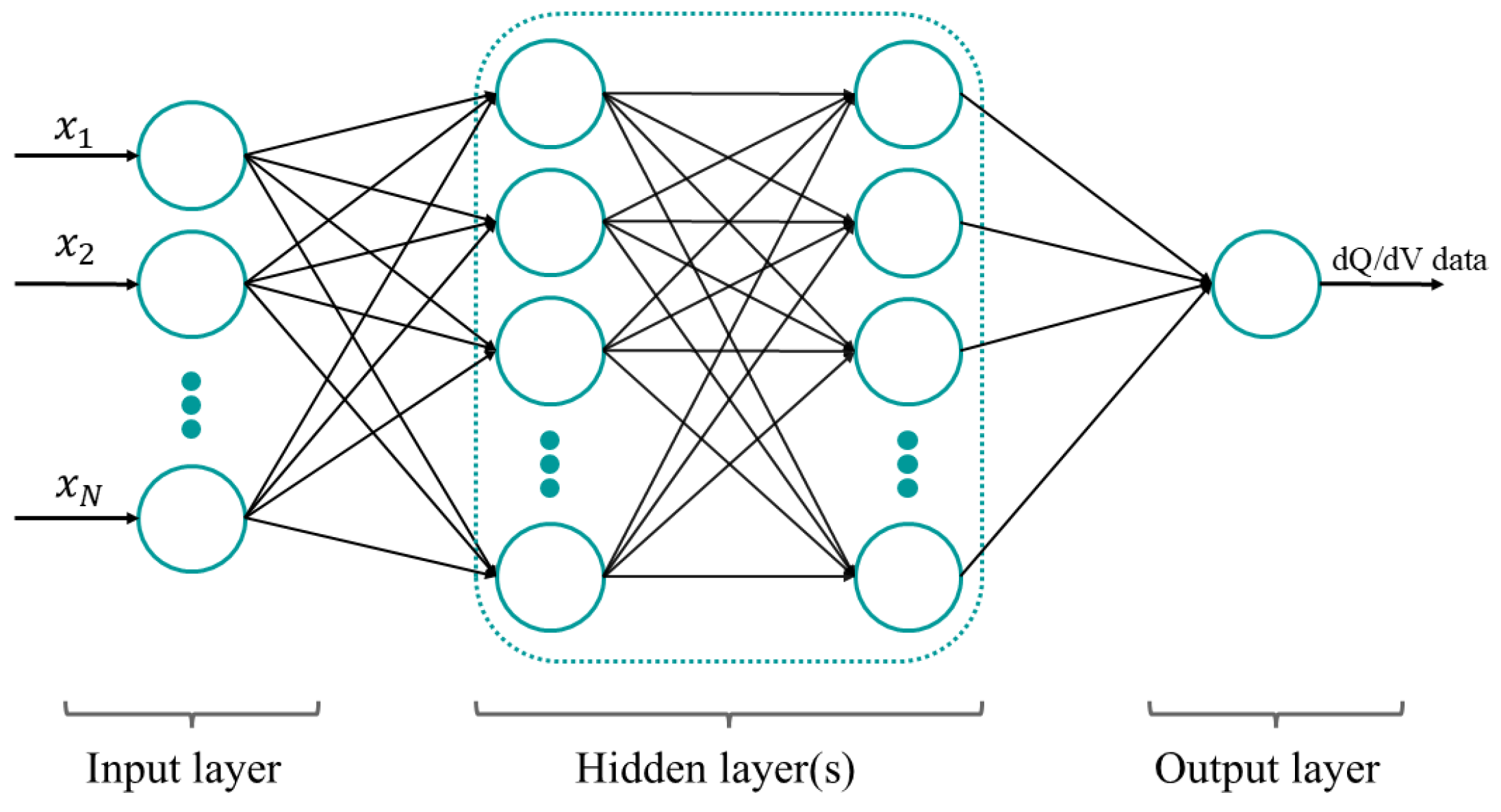
Figure 1. Simple schematic for a typical NN with two hidden layers. Here, x 1 to x N refer to the input data temperature, cycle number, and the 1C input data, and the output data are the differential capacity profiles.
Energies 17 04954 g001
Figure 2. Differential capacity profile for a 25 °C cycled cell, alongside the features of interest (FOI).
Energies 17 04954 g002
Figure 3. Differential capacity profile for a 35 °C cycled cell.
Energies 17 04954 g003
Figure 4. Differential capacity profile for a 45 °C cycled cell.
Energies 17 04954 g004
Figure 5. The performance metrics for predicting differential capacity profiles are illustrated, displaying the MSE (a) and MAE (b). It is noted that values at cycle 0 are not valid.
Energies 17 04954 g005
Figure 6. Scatter plot illustrating the comparison between actual and predicted values for differential capacity profile prediction using the FNN model (a), RNN model (b), and LSTM model (c).
Energies 17 04954 g006
Figure 7. Display of actual and predicted differential capacity analysis values obtained from the trained FNN model using the 45 °C evaluation dataset. Values corresponding to cycle 0 were excluded from the evaluation.
Energies 17 04954 g007
Figure 8. Display of actual and predicted differential capacity analysis values obtained from the trained RNN model using the 45 °C evaluation dataset. Values corresponding to cycle 0 were excluded from the evaluation.
Energies 17 04954 g008
Figure 9. Display of actual and predicted differential capacity analysis values obtained from the trained LSTM model using the 45 °C evaluation dataset. Values corresponding to cycle 0 were excluded from the evaluation.
Energies 17 04954 g009
Table 1. Hyperparametric search space in the random search method.
HyperparameterLower ValueUpper Value
Number of hidden layers13
Number of nodes per layer32516
Learning rate, α 10−410−2
Activation functionsLeaky ReLu, tanh
Table 2. Feed forward network architecture.
50 Outputs, α = 2.25 × 10⁻³
Layer TypeNodesActivation Function
Input layer101None
Dense64tanh
Dense288tanh
Dense416Leaky ReLu
Output layer50Linear
Table 3. Recurrent network architecture.
50 Outputs, α = 3.70 × 10⁻³
Layer TypeOutput ShapeActivation Function
SimpleRNN(none, 1, 64)tanh
SimpleRNN(none, 240)Leaky ReLu
Dense(none, 112)Leaky ReLu
Output layer50Linear
Table 4. Long short-term memory network architecture.
50 Outputs, α = 1.37 × 10⁻³
Layer TypeOutput ShapeActivation Function
LSTM(none, 1, 144)tanh
LSTM(none, 416)Leaky ReLu
Dense(none, 192)tanh
Output layer50Linear
Table 5. Performance measures (MSE and MAE) for the RNN, LSTM, and FNN in predicting differential capacity profiles.
FNNRNNLSTM
Evaluation SetMSEMAEMSEMAEMSEMAE
25 °C2.049.830.725.690.494.43
35 °C1.086.361.036.310.584.66
45 °C0.625.930.906.150.404.04
Evaluation score1.257.370.896.050.494.38
Time, range [ms]55–26649–13351–299
Disclaimer/Publisher’s Note: The statements, opinions and data contained in all publications are solely those of the individual author(s) and contributor(s) and not of MDPI and/or the editor(s). MDPI and/or the editor(s) disclaim responsibility for any injury to people or property resulting from any ideas, methods, instructions or products referred to in the content.