Abstract
This paper proposes a correction technique for bad data and high-precision analysis based on micro-phasor measurement unit (μPMU) data for a stable and reliable smart substation. First, a high-precision wide-area monitoring system (WAMS) with 35 μPMUs installed at Korea’s Yeonggwang substation, which is connected to renewable energy sources (RESs), is introduced. Time-synchronized μPMU data are collected through the phasor data concentrator (PDC). A pre-processing program is implemented and utilized to integrate the raw data of each μPMU into a single comma-separated values (CSV) snapshot file based on the Timetag. After presenting the technique for identification and correction of event, duplicate, and spike bad data of μPMU, causal relationships are confirmed through the voltage and current fluctuations for a total of five states, such as T/L fault, tap-up, tap-down, generation, and generation shutdown. Additionally, the difference in active power between the T/L and the secondary side of the M.Tr is compared, and the fault ride through (FRT) regulations, when the fault in wind power generation (WP), etc., occurred, is analyzed. Finally, a statistical analysis, such as boxplot and kernel density, based on the instantaneous voltage fluctuation rate (IVFR) is conducted. As a result of the simulation evaluation, the proposed correction technique and precise analysis can accurately identify various phenomena in substations and reliably estimate causal relationships.
1. Introduction
In order to monitor and analyze the existing power system, a supervisory control and data acquisition/energy management system (SCADA/EMS) is being operated. Since this SCADA/EMS provides monitoring information with a long data acquisition cycle of about once every 4 s for current, voltage, etc., and with unsynchronized standard time information, it is not precise and cannot recognize significant changes in the blind spot section. On the other hand, phase measurement units (PMUs) can collect accurate and time-synchronized electrical signals such as magnitude, phase angle, frequency, and rate of change of frequency (ROCOF) based on global positioning system (GPS) signals with a short data acquisition cycle of up to 256 times per cycle. Therefore, it can play a critical role because it can improve the accuracy of power system monitoring and real-time operation [1,2].
The Korea Electric Power Corporation (KEPCO) of Korea is promoting the construction and utilization of a next-generation intelligent transmission grid operation system to achieve its vision of building a world-class transmission grid operation platform. In the short term, SCADA and root mean square (RMS)-based renewable power generation capacity expansion and stable operation technology, as well as new and renewable power generation regional output prediction and control technology, are being developed. Therefore, based on transmission grid operation monitoring by the next-generation SCADA system, the transmission grid operation is expected to be optimally operated by using the digital twin transmission grid operation system through the exact diagnosis of the transmission grid operation by the PMU-based wide area monitoring system (WAMS) [3,4,5].
In accordance with the 3rd Basic Plan for Smart Power Grid, Korea’s PMU operation was expanded to 51 units in 36 substations centered around the metropolitan area in 2022, and plans are to install and expand to more than 200 PMUs by 2027. For a high-precision monitoring system, 19 PMUs were installed in 18 locations, including Jeju Island substations and Haenam and Jindo converter stations, which are high-voltage direct current (HVDC) connection points, to build J-WAMS by 2023 [5].
In related studies in Korea, data-driven synchro-phasor analysis using PMU big data for situational awareness of electric power grids [6], power system analysis using PMU and validating PMU data for calculating transformer % impedance [7], big data analysis of PMU for power quality of renewable energy sources (RESs) in the Gangwon area [8], system frequency based analysis and design of a fault ride through (FRT) detection system using PMU were presented [9]. In a study on a real-time system transient stability visualization method using PMU [10], advanced monitoring and detection of oscillation phenomena that may occur during system operation using PMU data in the Jeju power system was developed [11]. Recently, global digital substations, the latest time synchronization trends and application cases [12], digital substation IEEE 1588 time synchronization cases, and performance evaluation were introduced [13].
In related overseas studies, a micro-synchrophasor-based special protection scheme (SPS) for distribution system automation in a smart city [14], an islanding detection scheme (IDS) by Pearson’s correlation coefficient for islanding detection using μPMU measurements were proposed [15]. Synergizing PMU data from multiple locations in an Indian power grid case study [16], implementation of a WAMS for the power transmission grid of Bangladesh for monitoring the dynamic stability of the grid [17], parallel computing-based PMU measurements big data query tool to analyze the Colombian power system dynamic performance were analyzed [18]. Additionally, data-driven detection and identification of line parameters with PMU and unsynchronized SCADA measurements in distribution grids were published [19]. Recently, event detection and classification using machine learning applied to PMU data for the western United States power system [20] and application of power system wide-band oscillation monitoring and alarm systems based on PMU data [21] have been studied.
The purpose of this paper is to perform a high-precision analysis using large data collected from 35 μPMUs installed at Yeonggwang substation, which is connected to RESs, for a stable and reliable smart substation in Korea. After collecting the time-synchronized μPMU data through a phasor data concentrator (PDC), to shorten the time and facilitate data analysis, the data from each of 35 μPMUs were pre-processed in the form of snapshots by integrating electrical signals such as voltage, current, etc., based on the Timetag. A technique for the identification and correction of event, duplicate, and spike bad data of μPMU is proposed. Causal relationships are confirmed through the voltage and current fluctuations for a total of five states, such as T/L fault, tap-up, tap-down, generation, and generation shutdown. Additionally, the difference in active power between the T/L and the secondary side of the M.Tr is compared, and the FRT regulations, when the fault in wind power generation (WP), etc., occurred, is analyzed. Finally, we intended to perform statistical analyses such as boxplots and kernel density based on the instantaneous voltage fluctuation rate (IVFR).
The remainder of this paper is organized as follows. Section 2 describes the high-precision WAMS and μPMU data of the substation. Section 3 explains the bad data detection and the correction technique. Section 4 describes the μPMU data-based high-precision analysis, and we summarize and discuss all the results we have achieved. Finally, the conclusions are highlighted in the Section 5.
2. High-Precision WAMS and μPMU Data of the Substation
2.1. High-Precision WAMS of the Substation
The Yeonggwang substation WAMS in the Jeonnam Province of Korea has 35 μPMUs installed, which are connected to RESs. Figure 1 shows a single-line diagram of the Yeonggwang substation [2]. As shown in Figure 1, ① T/L zone consists of Jangseong-Yeonggwang #1 T/L, Jangseong-Yeonggwang #2 T/L, Gochang-Yeonggwang T/L, Yeonggwang-Hongnong T/L, Baeksu WP T/L, Jaewon photovoltaic (PV) T/L, Hamgumi PV T/L, and #1 Sh.C. ② The 154 kV bus zone is composed of buses #60 and #61 that are connected to ① T/L zone. M.Tr is composed of a total of 4 zones, each of which is divided into ③ M.Tr primary side (154 kV) zone and ④ M.Tr secondary side (23 kV) zone. ⑤ The 23 kV bus zone is composed of buses #40∼#43 and #45∼#48 that are connected to the ⑥ D/L zone. ⑥ The D/L zone consists of 25 distribution lines connected to loads, power plants, STR, and Sh.C.
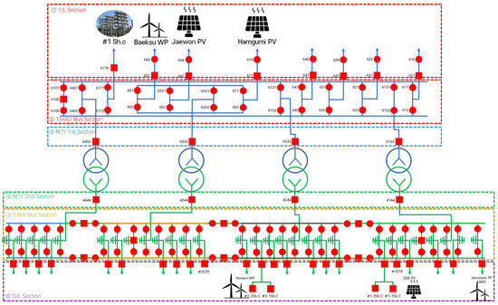
Figure 1.
A single-line diagram of the Yeonggwang substation.
Table 1 shows the RESs connected to the Yeonggwang substation. As shown in Table 1, the 154 kV area was connected to Baeksu WP, Jaewon PV, and Hamgumi PV. The 22.9 kV area was connected to Honam WP, DSE (PV), and Jeonnam TP (WP).

Table 1.
The RESs connected to the Yeonggwang substation.
Table 2 shows the monitoring points of the Yeonggwang substation WAMS. As shown in Table 2, μPMUs are installed at all monitoring points except for some newly established D/L.

Table 2.
The monitoring point of the Yeonggwang substation WAMS.
2.2. μPMU Data Collection and Pre-Processing
The μPMU data stored at the substation is saved as a comma-separated values (CSV) format file through μPMU’s internal calculation process. Figure 2 shows the structure of the raw data of the Yeonggwang substation. As shown in Figure 2, the CSV files saved from 35 μPMUs are all based on the same 1-cycle periodic Timetag for 24 h starting from 00:00:00 on the day of collection. The 23 items of the data are collected, such as μPMU ID, state, frequency, frequency change rate, and time-synchronized phasor of the three-phase voltage and current. That is, the raw data are saved daily as 35 CSV files of 5,184,000 × 23 size.
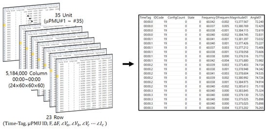
Figure 2.
The structure of the raw data of the Yeonggwang substation.
However, because the size of the raw data of each of the 35 CSV files is very large, it cannot be read by commercial programs. In addition, in order to obtain the desired information through analysis and comparison, it is cumbersome to read each CSV file of 35 μPMUs individually, and it takes a lot of time. Accordingly, we implemented a pre-processing conversion program using the Python 3.11.9 language to easily check the μPMU data [2]. The pre-processing is performed to integrate data collected from 35 μPMUs over time and convert them into a snapshot-type data structure based on the Timetag for each day’s raw data. Therefore, the raw data of 35 μPMUs with a size of 5,184,000 × 23 are integrated every day and built into 6 CSV files. The 6 files are reorganized by voltage magnitude, voltage phase, current magnitude, current phase, frequency, and frequency change rate. Therefore, a total of 6 integrated CSV files are built, one for each day in the month.
3. Bad Data Detection and Correction Technique
3.1. Correction Technique and Event Identification
In general, the raw data of μPMU has a small slope during the normal state. However, it has a high slope when an event such as a T/L fault, tap change, generation, and generation shutdown state occurs or when there is bad data. In particular, most bad data exist alone, and the number of consecutive bad data is three or less. Accordingly, we proposed the identification and correction technique for bad data using slope and count. The slope ( of each raw data is calculated by Equation (1).
where, represent the μPMU raw data at the and sample point, respectively. represent the time at the and sample point, respectively, t represents the 1 cycle.
Figure 3 shows the flowchart of the correction technique for bad data. As shown in Figure 3, first, μPMU raw data are read. Calculate the slope ( of each raw data using Equation (1). If the slope of each raw data is 0, increase the duplicate count (. Otherwise, the slope of each raw data is greater than the threshold1 (TH1), the spike count () is increased. Otherwise, if there are more than 3 duplicate counts, it is identified as duplicate data, and then the average of the data of the same bus in the corresponding time period is calculated to replace and correct the duplicate data. Otherwise, if the spike count is 1, it is identified as an event such as a T/L fault, tap-up, and tap-down state. If the spike count is 2, the spike slope is calculated, and if it exceeds the threshold2 (TH2), it is identified as a spike and corrected by Equation (2). If it does not exceed, it is identified as an event. If the spike count is 3, the spike slope is calculated, and if it exceeds the TH2, it is identified as a spike and corrected by Equations (3) and (4). If not, it is identified as an event. In this paper, through various case studies, the settings of TH1 and TH2 were 200 and 10,000, respectively.
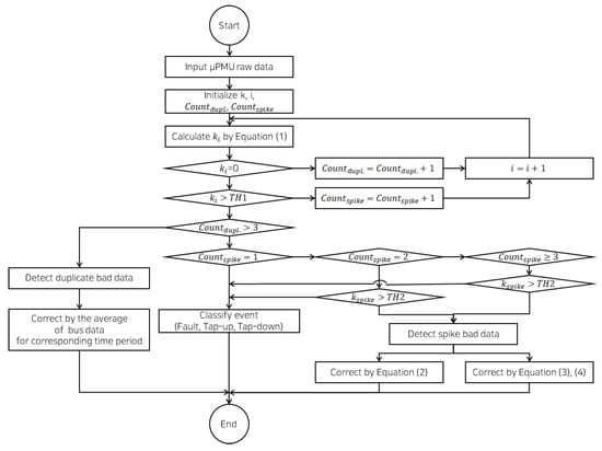
Figure 3.
The flowchart of the correction technique for bad data.
3.2. Correction of Duplicate Bad Data
Figure 4 shows the duplicate bad data and corrected data. As shown in Figure 4a, [Magnitude 011], [Magnitude 012], and [Magnitude 013] are the phase A data of the μPMU 11, 12, and 13. However, [Magnitude 013], the phase A data of the μPMU 13, shows the duplicated voltage values in the red section. According to the correction technique proposed, the duplicate bad data of [Magnitude 013] was replaced with a blue section after calculating the average value of the same bus data, as shown in Figure 4b.
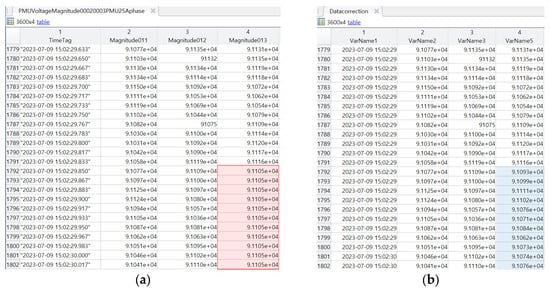
Figure 4.
The duplicate bad data and corrected data: (a) bad data; (b) corrected data.
3.3. Correction of Spike Bad Data
Figure 5 shows the spike bad data and corrected data. As shown in Figure 5a, one sample (566th) of [Magnitude 014], the phase A data of the μPMU 14, momentarily showed a small voltage value, as shown in the red section. In other words, it shows the spike bad data. According to the correction technique proposed, the spike bad data of one sample (566th) was replaced with a blue section after calculating the average value of data of one sample (565th) and one sample (567th) of the same the μPMU 14, as shown in Figure 5b.

Figure 5.
The spike bad data and corrected data: (a) bad data; (b) corrected data.
4. μPMU Data Based High-Precision Analysis
We extracted one hour of the voltage and current data using a system phenomena analysis program implemented in Python 3.11.9 and then examined the voltage and current fluctuations and fluctuation periods.
4.1. Analysis of System Phenomena
The system phenomena observed in the μPMU data of the substation can be categorized into five types such as T/L fault, tap-up and down of M. Tr, generation, and generation shutdown.
4.1.1. T/L Fault State
The T/L fault state indicates a three-phase auto-reclosing operation due to the T/L fault in this paper. Figure 6 shows the voltage and current of some sections during the T/L fault state. As shown in Figure 6, the T/L fault occurred on 10 July 2023 from 06:02:47.0 to 06:02:47.6. During the 6 cycles of 100.000 ms of the T/L fault state, the results of checking the 1 min data showed that the voltages of phase A, phase B, and phase C decreased from 90.529 kV, 91.870 kV, and 90.895 kV to 79.079 kV, 88.680 kV, and 86.088 kV, respectively, by 11.450 kV (12.878%), 3.190 kV (3.588%), and 4.807 kV (5.406%). During the T/L fault occurred the currents of phases A, B, and C increased from 85.959 A, 87.723 A, and 74.603 A to 206.994 A, 76.538 A, and 114.972 A, respectively, by 121.035 A (26.904%), 11.185 A (2.486%), and 40.369 A (8.973%).

Figure 6.
The voltage and current during the T/L fault state.
Table 3 shows the occurrence history of the T/L faults for a total of 7 days from 10 July to 16 July 2023. Using the system phenomena analysis program to check 1 min data, a total of the 23 T/L faults were easily detected over a 7-day period.

Table 3.
The T/L fault history.
4.1.2. Tap-Up State
Figure 7 shows the voltage and current during the tap-up state. As shown in Figure 7, the M.Tr tap-up operation happened on 24 July 2023 from 07:26:24.9 to 07:26:25.4. During the 4 cycles of 66.667 ms of the tap-up state, the results of checking the 1 min data showed that the voltages of phases A, B, and C increased from 13.188 kV, 13.301 kV, and 13.262 kV, respectively, to 13.343 kV, 13.457 kV, and 13.421 kV, respectively, by 155.170 V (1.174%), 156.240 V (1.182%), and 158.940 V (1.202%). During the M. Tr tap-up, the currents of phases A, B, and C increased from 189.803 A, 195.393 A, and 191.196 A to 193.726 A, 199.963 A, and 196.463 A, respectively, by 3.923 A (0.259%), 4.570 A (0.302%), and 5.267 A (0.348%).

Figure 7.
The voltage and current during the tap-up state.
4.1.3. Tap-Down State
Figure 8 shows the voltage and current during the tap-down state. As shown in Figure 8, the M.Tr tap-down operation happened on 27 July 2023 from 16:26:22.5 to 16:26:23.4. During the 5 cycles of 83.333 ms of the tap-down state, the results of checking the 1 min data showed that the voltages of phases A, B, and C decreased from 13.514 kV, 13.535 kV, and 13.515 kV, respectively, to 13.353 kV, 13.377 kV, and 13.357 kV, respectively, by 161.510 V (1.222%), 158.170 V (1.196%), and 157.930 V (1.195%). During the M.Tr tap-down, the currents of phases A, B, and C increased from 111.405 A, 114.615 A, and 119.391 A to 107.722 A, 117.051 A, and 127.142 A, respectively, by 3.683 A (0.243%), 2.436 A (0.161%), and 7.751 A (0.512%).

Figure 8.
The voltage and current during the tap-down state.
4.1.4. Generation State
Figure 9 shows the voltage and current during the generation state. As shown in Figure 9, the generation happened on 10 July 2023 from 06:28:50.8 to 06:28:51.4. During the generation state, the results of checking the 1 min data showed that the voltages of phases A, B, and C fluctuated slightly from 13.303 kV, 13.363 kV, and 13.300 kV to 13.299 kV, 13.357 kV, and 13.305 kV, respectively, by 3.550 V (0.027%), 6.260 V (0.047%), and 5.760 V (0.044%). During the generation, the current of phase A, phase B, and phase C increased from 0 A, 0 A, and 0 A to 0 A, 5.949 A, and 0 A, respectively, by 0 A (0.000%), 5.949 A (0.393%), and 0 A (0.000%). However, only the phase B current increased from 0 A to approximately 5.949 A.

Figure 9.
The voltage and current during the generation state.
4.1.5. Generation Shutdown State
Figure 10 shows the voltage and current during the generation shutdown state. As shown in Figure 10, the generation shutdown happened on 10 July 2023 from 19:27:21.2 to 19:27:21.8. During the generation shutdown state, the results of checking the 1 min data showed that the voltages of phases A, B, and C slightly fluctuated by 3.000 V (0.023%), 4.000 V (0.030%), and 6.000 V (0.045%) from 13.351 kV, 13.351 kV, and 13.300 kV to 13.354 kV, 13.347 kV, and 13.294 kV, respectively. During the generation shutdown, the current of phases A, B, and C decreased by 5.824 A (0.385%), 0 A (0.000%), and 6.121 A (0.405%) from 5.824 A, 0 A, and 6.121 A to 0 A, 0 A, and 0 A, respectively. However, only the current of phases A and C decreased from 5.824 A to 6.121 A to 0 A, respectively.

Figure 10.
The voltage and current during the generation shutdown state.
As a result of analyzing various cases, the T/L fault state had a duration of more than 6 cycles, the three-phase voltage decreased by at least 3% or more compared to the rated voltage, and the three-phase current increased by at most 26% compared to the rated current. The tap-up state had a duration of 4 cycles, the three-phase voltage increased by 1.186% compared to the rated voltage, and the three-phase current increased less by 0.303% compared to the rated current. The tap-down state had a duration of 5 cycles, the three-phase voltage decreased by 1.204% compared to the rated voltage, and the three-phase current increased by 0.143% compared to the rated current. In the generation state, the three-phase voltage and current gradually increased over a long duration of time, and the current changed from 0 A to (+). In the generation shutdown state, the three-phase voltage and current gradually decreased over a long duration of time, and the current changed from (+) to 0 A. Therefore, it was possible to identify five system phenomena in the substation.
4.2. Comparison of Active Power Difference
To investigate the condition of the substation components, the active power is calculated and analyzed using the magnitude and phase angle of the voltage and current based on μPMU integrated data. Figure 11 shows the active power comparison between T/L and the secondary side of M.Tr. These two positions were selected because the CT was not installed on the primary side of the M.Tr in Figure 11, making it impossible to measure the current [2]. The loss of the T/L bus is expected to be small, but the difference in active power between T/L and the secondary sides of the M.Tr was compared.
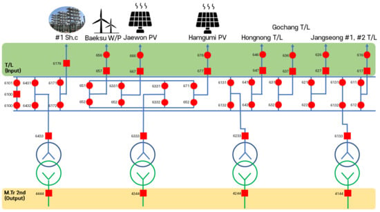
Figure 11.
The active power comparison of the T/L and secondary side of the M.Tr.
4.2.1. T/L Fault State
Figure 12 shows the active power comparison during a three-phase auto-reclosing operation due to the T/L fault state in this paper. As shown in Figure 12, the T/L fault occurred on 11 July 2023 from 11:02:15.4 to 11:02:24.0, the average active power of T/L was −53.168 MW, the average active power of the secondary side of M.Tr was 57.279 MW; therefore, the average of the active power difference was 4.111 MW (2.284%). During the 84 cycles of 1.400 s of the T/L fault, the active power difference was found to be the largest at 43.915 MW (24.398%) at 20.083 s.
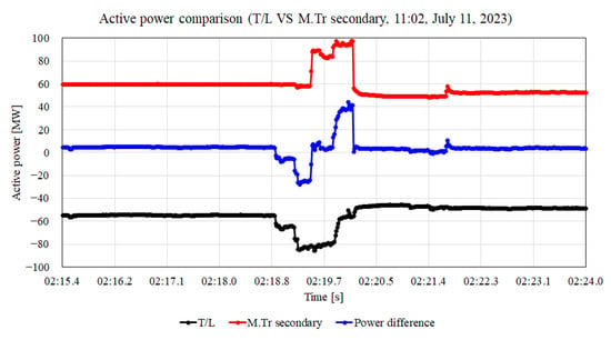
Figure 12.
The active power comparison during the T/L fault state.
4.2.2. Tap-Up State
Figure 13 shows the active power comparison during the tap-up state. As shown in Figure 13, the M.Tr tap-up operation happened on 14 July 2023 from 08:42:00.0 to 08:42:43.2, and the average active power of the T/L side was −24.385 MW; therefore, the average active power of the secondary side of the M.Tr was 15.455 MW, and the average active power difference was small, at approximately −8.930 MW (4.961%).
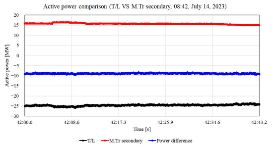
Figure 13.
The active power comparison during the tap-up state.
4.2.3. Tap-Down State
Figure 14 shows the active power comparison during the tap-down state. As shown in Figure 14, the M.Tr tap-down operation happened on 13 July 2023 from 01:53:02.4 to 01:53:54.2, the average active power of the T/L side was −14.745 MW, and the average active power of the secondary side of the M.Tr was 8.620 MW, which includes noise compared to other phenomena. Therefore, the average active power difference was small, approximately −6.125 MW (3.403%), similar to the tap-up.
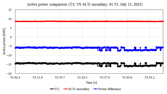
Figure 14.
The active power comparison during the tap-down state.
4.2.4. Generation State
Figure 15 shows the active power comparison during the generation state. As shown in Figure 15, the generation happened on 11 July 2023 from 07:51:01.4 to 07:51:53.3. The average active power of the T/L side was −18.296 MW, and the average active power of the secondary side of the M.Tr was 9.356 MW; therefore, the average active power difference was approximately −8.940 MW (4.967%).
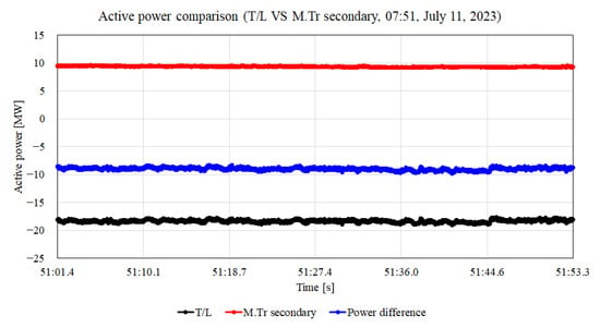
Figure 15.
The active power comparison during the generation state.
4.2.5. Generation Shutdown State
Figure 16 shows the active power comparison during the generation shutdown state. As shown in Figure 16, the generation shutdown happened on 15 July 2023 from 18:31:06.2 to 18:31:45.1. The average active power of the T/L side was −12.576 MW, and the average active power of the secondary side of the M.Tr was 7.888 MW, showing an oscillating phenomenon. Therefore, the average active power difference was approximately −4.688 MW (2.604%).
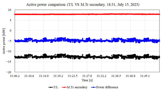
Figure 16.
The active power comparison during the generation shutdown state.
4.3. Analysis of FRT Regulations
Among the RESs linked to the substation, WP was analyzed to determine whether it complies with the FRT regulations. Figure 17 shows the FRT regulations in Korea [22]. When a system fault occurs, the voltage must be restored to 50% or more within 150 ms, and the linked operation must be maintained at 80% or more for up to 1000 ms. After 1000 ms, the generator may be disconnected.
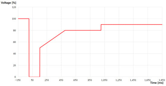
Figure 17.
The FRT regulations in Korea.
4.3.1. Baeksu WP
Figure 18 shows the voltage during the fault at T/L connected to the Baeksu WP that occurred on 11 July 2023 from 13:39:36.5 to 13:39:37.9 according to the FRT regulations. As shown in Figure 18, the voltages of phases A, B, and C decreased to 86.504 kV at the time of the fault but continued to maintain operation. According to the domestic FRT regulations, the voltage recovered to 50% within 150 ms and to 80% within 500 ms after the fault occurred, and the grid-connected operation was maintained well for up to 1000 ms. This shows that the system precisely met the FRT regulations.
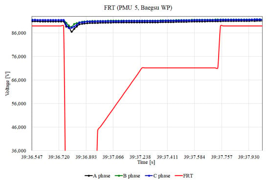
Figure 18.
The voltage during the Baegsu WP T/L fault according to the FRT regulations.
4.3.2. Honam WP
Figure 19 shows the voltage during the fault at D/L connected to the Honam WP that occurred on 11 July 2023 from 13:39:36.5 to 13:39:37.9. As shown in Figure 19, the voltages of phases A, B, and C decreased to 12.579 kV at the time of the fault but continued to maintain operation. This shows that the system precisely met the FRT regulations.
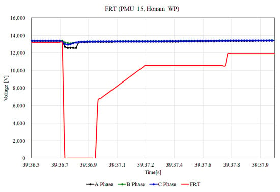
Figure 19.
The voltage during the Honam WP D/L fault according to the FRT regulations.
4.3.3. Jeonnam TP (WP)
Figure 20 shows the voltage during the fault at D/L connected to the Jeonnam TP (WP) that occurred on 11 July 2023 from 13:39:36.5 to 13:39:37.9. As shown in Figure 20, the voltages of phases A, B, and C decreased to 12.575 kV at the time of the fault but continued to maintain operation. This shows that the system precisely met the FRT regulations.
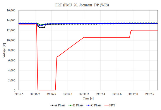
Figure 20.
The voltage during the Jeonnam TP (WP) D/L fault according to the FRT regulations.
4.4. Instantaneous Voltage Fluctuation Rate-Based Statistical Analysis
IVFR was used as analysis data for statistical techniques. Equation (5) represents the IVFR calculation formula. In Equation (5), the IVFR calculates the difference between the maximum and minimum values of the effective voltage as a percentage of the nominal voltage of the system using a moving window of 12 cycles in size. The IVFR is used in statistical techniques such as boxplot and kernel density.
According to Korea’s distributed power distribution system interconnection technology standards, the IVFR is applied so that it does not exceed 3% [2].
4.4.1. Boxplot
Boxplot is a statistical technique used to visualize data distribution. Boxplots can be used to identify the distribution of data, median, and outliers. Figure 21 shows the structure of the boxplot. As shown in Figure 21, the boxplot visualizes the interquartile range (IQR), which is the difference between the upper and lower quartiles of the data. Boxplots check for outlier values that fall outside the normal range and whether the grid voltage is maintained at a certain level.
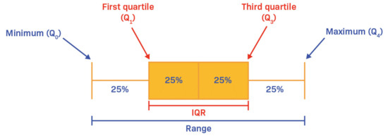
Figure 21.
The structure of the boxplot.
T/L Fault State
Figure 22 shows the results of boxplot analysis during the T/L fault state, as shown in Figure 6. As shown in Figure 22, the maximum values of IVFR of phases A, B, and C were 4.941%, 4.423%, and 4.824%, and the third quartiles were 0.065%, 0.066%, and 0.063%, and the medians were 0.054%, 0.054%, and 0.053%. It can be seen that the tolerance for IVFR has been exceeded by 3%. Therefore, the three-phase average of IVFR during the T/L fault duration was more than 4%, and the three-phase average of the third quartile and the median were 0.065% and 0.054%, respectively, identifying a similar distribution.
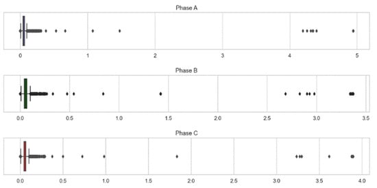
Figure 22.
The results of boxplot analysis during the T/L fault state.
Table 4 shows the results of boxplot analysis during the T/L fault state of the date of occurrence. As shown in Table 4, the maximum values of the three-phase averages of IVFR ranged from 2.262% to 6.257%, the three-phase averages of third quartiles ranged from 0.066% to 0.072%, and three-phase averages of the medians ranged from 0.053% to 0.061%. In some cases, it can be identified that the tolerance for IVFR during the T/L fault duration has been exceeded by 3%. The three-phase average of the third quartile and the median were 0.069% and 0.056%, respectively, identifying no fluctuations.

Table 4.
The results of boxplot analysis during the T/L fault state of the date of occurrence.
Tap-Up State
Figure 23 shows the results of boxplot analysis during the tap-up state, as shown in Figure 7. As shown in Figure 23, the maximum values of IVFR of phases A, B, and C were 1.284%, 1.272%, and 1.293%, the third quartiles were 0.065%, 0.066%, and 0.063%, and the medians were 0.054%, 0.054%, and 0.053%. It can be seen that the tolerance for IVFR has not been exceeded by 3%.
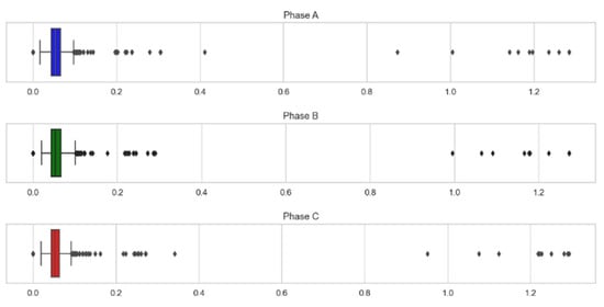
Figure 23.
The results of boxplot analysis during the tap-up state.
Table 5 shows the results of boxplot analysis during the tap-down state of the date of occurrence. As shown in Table 5, the maximum values of the three-phase averages of IVFR ranged from 1.186% to 2.498%, the three-phase averages of third quartiles ranged from 0.046% to 0.105%, and the three-phase averages of medians ranged from 0.035% to 0.088%. Therefore, the three-phase average of IVFR was 1.340%. It can be identified that the tolerance for IVFR during the tap-up duration has not been exceeded by 3%. The three-phase average of the third quartile and the median were 0.069% and 0.057%, respectively, identifying no fluctuations.

Table 5.
The results of boxplot analysis during the tap-up state of the date of occurrence.
Tap-Down State
Figure 24 shows the results of boxplot analysis during the tap-down state, as shown in Figure 8. As shown in Figure 24, the maximum values of the IVFR of phases A, B, and C were 1.222%, 1.248%, and 1.231%, the third quartiles were 0.074%, 0.073%, and 0.077%, and the medians were 0.060%, 0.059%, and 0.061%. It can be seen that the tolerance for IVFR has not been exceeded by 3%.
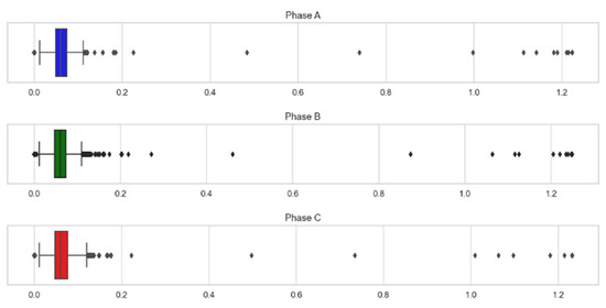
Figure 24.
The results of boxplot analysis during the tap-down state.
Table 6 shows the results of boxplot analysis during the tap-down state of the date of occurrence. As shown in Table 6, the maximum values of the three-phase averages of IVFR ranged from 1.185% to 1.312%, the three-phase averages of third quartiles ranged from 0.049% to 0.104%, and the three-phase averages of medians ranged from 0.039% to 0.091%. Therefore, the three-phase average of IVFR was 1.237%. It can be identified that the tolerance for IVFR has not been exceeded by 3%. The three-phase average of the third quartile and the median were 0.071% and 0.059%, respectively. The three-phase average of the third quartile and the median were 0.071% and 0.059%, respectively, identifying no fluctuations, similar to the tap-up.

Table 6.
The results of boxplot analysis during the tap-down state of the date of occurrence.
Generation State
Figure 25 shows the results of boxplot analysis during the generation state, as shown in Figure 9. As shown in Figure 25, the maximum values of the IVFR of phases A, B, and C were 0.092%, 0.135%, and 0.062%, the third quartiles were 0.017%, 0.013%, and 0.012%, and the medians were 0%. It was found to satisfy the 3% tolerance for IVFR.
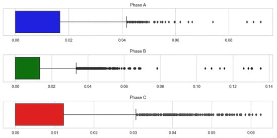
Figure 25.
The results of boxplot analysis during the generation state.
Table 7 shows the results of boxplot analysis during the generation state of the date of occurrence. As shown in Table 7, the maximum values of the three-phase averages of IVFR ranged from 0.119% to 0.211%, the three-phase averages of third quartiles ranged from 0.017% to 0.099%, and the three-phase averages of medians ranged from 0.000% to 0.087%. Therefore, the three-phase average of IVFR was 0.154%. It can be identified that the tolerance for IVFR has not been exceeded by 3%. The three-phase average of the third quartile and the median were 0.064% and 0.051%, respectively, identified as small.

Table 7.
The results of boxplot analysis during the generation state of the date of occurrence.
Generation Shutdown State
Figure 26 shows the results of boxplot analysis during the generation shutdown state, as shown in Figure 10. As shown in Figure 26, the maximum values of the IVFR of phases A, B, and C were 0.114%, 0.117%, and 0.100%, the third quartiles were 0.062%, 0.060%, and 0.067%, and the medians were 0.051%, 0.047%, and 0.054%. It was found to satisfy the 3% tolerance for IVFR.
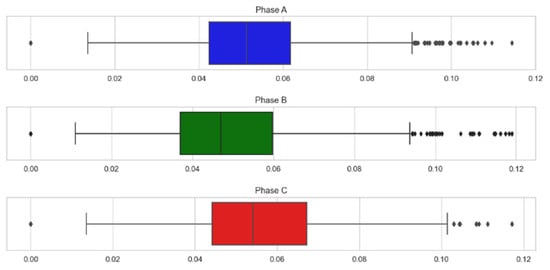
Figure 26.
The results of boxplot analysis during the generation shutdown state.
Table 8 shows the results of the boxplot analysis during the generation shutdown state of the date of occurrence. As shown in Table 8, the maximum values of the three-phase averages of IVFR ranged from 0.101% to 0.178%, the three-phase averages of third quartiles ranged from 0.045% to 0.077%, and the three-phase averages of medians ranged from 0.035% to 0.061%. Therefore, the three-phase average of IVFR was 0.131%. It can be identified that the tolerance for IVFR has not been exceeded by 3%. The three-phase average of the third quartile and the median were 0.058% and 0.047%, respectively, identifying no fluctuations, similar to the generation.

Table 8.
The results of boxplot analysis during the generation shutdown of the date of occurrence.
4.4.2. Kernel Density
Kernel density estimation (KDE) is a non-parametric density estimation method that improves upon the issues of the histogram method by using a kernel function. Mathematically, a kernel function is defined as a non-negative function that is symmetric about the origin and has an integral value of 1.
T/L Fault State
Figure 27 shows the results of kernel density analysis during the T/L fault state, as shown in Figure 6. As shown in Figure 27, the maximum values of kernel density of phases A, B, and C were 13.825 at 0.054%, 13.338 at 0.054%, and 13.177 at 0.046%. Therefore, all phases A, B, and C show a very low average IVFR of 0.051% and a very high density of 13.447.
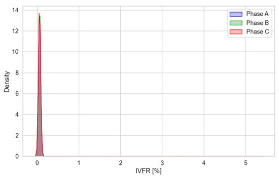
Figure 27.
The results of kernel density during the T/L fault state.
Tap-Up State
Figure 28 shows the results of kernel density analysis during the tap-up state, as shown in Figure 7. As shown in Figure 28, the maximum values of kernel density of phases A, B, and C were 18.601 at 0.050%, 19.102 at 0.050%, and 20.070 at 0.050%. Therefore, all phases A, B, and C show a very low average IVFR of 0.050% and a very high density of 19.258.
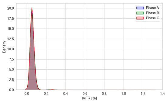
Figure 28.
The results of kernel density during the tap-up state.
Tap-Down State
Figure 29 shows the results of kernel density analysis during the tap-down state, as shown in Figure 8. As shown in Figure 29, the maximum values of kernel density of phases A, B, and C were 17.151 at 0.064%, 16.768 at 0.062%, and 16.061 at 0.060%. Therefore, all phases A, B, and C show a very low average IVFR of 0.062% and a very high density of 16.660, similar to the tap-down.
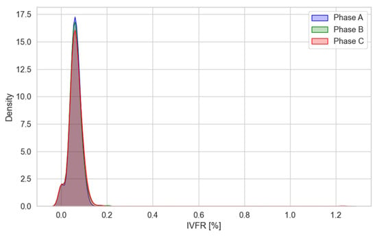
Figure 29.
The results of kernel density during the tap-down state.
Generation State
Figure 30 shows the results of kernel density analysis during the generation state, as shown in Figure 9. As shown in Figure 30, the maximum values of kernel density of phases A, B, and C were 95.054, 88.301, and 75.321 at 0%. Therefore, all phases A, B, and C show a very low average IVFR of 0% and a very high density of 86.225.
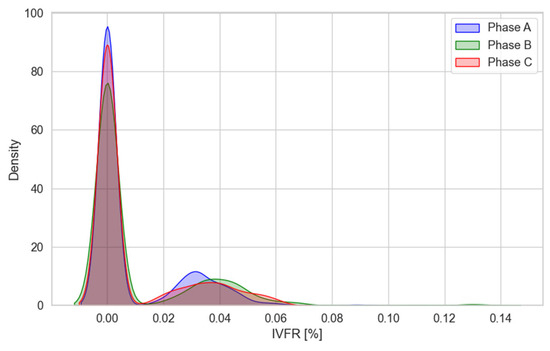
Figure 30.
The results of kernel density during the generation state.
Generation Shutdown State
Figure 31 shows the results of kernel density analysis during the generation shutdown state, as shown in Figure 10. As shown in Figure 31, the maximum values of kernel density of phases A, B, and C were 27.735 at 0.049%, 26.952 at 0.045%, and 25.071 at 0.050%. Therefore, all phases A, B, and C show a very low average IVFR of 0.048% and a very high density of 26.586.
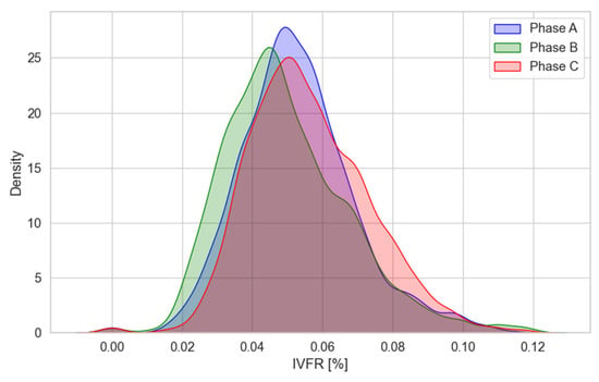
Figure 31.
The results of kernel density during the generation shutdown state.
4.5. Results and Discussion
Table 9 presents a summary of the research content and results on high-precision analysis using μPMU data for smart substations performed in this paper. As shown in Table 9, we proposed and implemented a pre-processing conversion program to enable operators to conveniently process and analyze 35 μPMU raw data. We proposed the slope and count of difference data-based technique to detect bad data, compensated the bad data satisfactorily, and identified events through the average-based correction technique. By implementing a system phenomenon analysis program, we investigated five system phenomena of voltage and current fluctuations and fluctuation periods for high-precision analysis based on μPMU data. As a result, in the T/L fault state, the duration was 6 cycles, the average voltage decreased to 6.482 kV (7.291%), the average current increased to 50.073 A (11.130%), and the program was able to find the automatic reclosing phenomenon. In the tap-up state, the duration was 4 cycles, the average voltage increased to 156.783 V (1.186%), and the average current decreased to 4.587 A (0.303%). In the tap-down state, the duration was 5 cycles, the average voltage decreased to 159.203 V (1.204%), and the average current increased to 2.168 A (0.143%). In the generation state, the duration was long, the average voltage increased to 1.150 V (0.010%), and the average current increased to 5.949 A (0.393%). In the generation shutdown state, the duration was long, the average voltage increased to 2.333 V (0.018%), and the average current decreased to 3.982 A (0.395%). Using the data between the T/L side and the secondary side of M.Tr, the active power between the input and output of the substation was analyzed. As a result, the active power in the T/L fault, tap-up, tap-down, generation, and generation shutdown states showed differences of 43.915 MW (24.398%), 8.930 MW (4.961%), 6.125 MW (3.403%), 8.940 MW (4.967%), and 4.688 MW (2.604%), respectively. That is, the differences in the active power during the occurrence of five phenomena were calculated. When the T/L and D/L faults occurred in WP and TP of the RES-linked substations, the allowable standards FRT regulations of Korea were checked and found to be satisfactory. Also, in the T/L fault at Baeksu WP, D/L fault at Honam WP, and Jeonnam TP (WP), the voltage showed decreases to 86.504 kV (97.292%), 12.579 kV (95.142%), 12.575 kV (95.112%), respectively. Finally, in order to verify compliance with Korea’s distributed power distribution system interconnection technology standards, the data distribution of the five phenomena was reconfirmed through analysis using the IVFR-based boxplot method. Additionally, in the T/L fault, tap-up, tap-down, generation, and generation shutdown, the average maximum values of IVFR were 3.804%, 1.340%, 1.237%, 0.154%, and 0.131%, respectively. Furthermore, the non-parametric density of each phenomenon was estimated using the IVFR-based kernel density. The densities for the T/L fault, tap-up, tap-down, generation, and generation shutdown were 13.447, 19.258, 16.660, 86.225, and 26.586, respectively.

Table 9.
The summary of the research contents, results, and implications.
In summary, an analysis program was implemented using Python 3.11.9 language for high-precision analysis by μPMU data for the entire components of the substation. All results can be applied to analyze causal relationships of various power system phenomena through a high-precision monitoring system of a smart substation with installed μPMU.
5. Conclusions
In order to build a stable and reliable smart substation, we have performed the first study utilizing large data of time-synchronized phasor data after installing 35 μPMUs at the 154 kV Yeonggwang substation in Korea.
First, we investigated μPMU-based high-precision at the WAMS of the Yeonggwang substation. The time-synchronized μPMU raw data collected through PDC were pre-processed into snapshot form by merging the voltage, current, etc., of 35 data based on Timetag, making data processing easier and reducing the time required for analysis. Events, duplicates, and spike bad data in μPMU were identified and corrected using the slope and count-based identification technique and the average-based correction technique. By implementing the proposed system phenomena analysis program, five phenomena were precisely analyzed by analyzing the magnitude and duration of voltage and current, such as T/L fault, tap-up, tap-down, generation, and generation shutdown. The difference in active power between the input and output of the substation was compared and calculated, and the Korean FRT regulations were reviewed under various conditions, including T/L and D/L faults in RESs connection lines, and it was found that they were all satisfied. Finally, regarding the Korean distributed distribution system interconnection technology standards, to reconfirm the data distribution of five phenomena related to substations, statistical analyses such as boxplot and kernel density based on IVFR were performed, and non-parametric densities were estimated.
In conclusion, the proposed correction technique and precise analysis can help iden-tify various phenomena in substation and estimate reliable causal relationships. In the near future, we plan to collect and utilize Comtrade data of several cases of faults in real fields to demonstrate its versatility and reliability.
Author Contributions
Investigation, K.-M.L.; writing—original draft, C.-W.P. All authors have read and agreed to the published version of the manuscript.
Funding
This research was funded by Korea Electric Power Corporation (Korea) grant number R22XO05-04.
Data Availability Statement
The original contributions presented in the study are included in the article, further inquiries can be directed to the corresponding author.
Conflicts of Interest
The authors declare no conflict of interest.
References
- Yun, S.Y.; Hong, J.S. Technical Trends of PMU Applications in Power Distribution Networks. Korean Inst. Electr. Eng. 2020, 69, 29–33. [Google Scholar]
- Park, C.W.; Lee, K.M.; Kim, K.M.; Lee, H.S.; Choi, Y.S.; Heo, Y.H.; Kim, T.H.; Jeon, D.H.; Jo, C.Y. Basic Study on Utilization Plan of PMU Data for 154kV Substation; 1st Year Report; KEPCO: Naju-si, Republic of Korea, 2023; pp. 1–163. [Google Scholar]
- KEPRI. Intelligent Power Grid Operation System. In External Open Basic Research Project Planning Advisory Meeting; KEPRI: Batam, Indonesia, 2023; pp. 1–24. [Google Scholar]
- KEPCO. Long-term Transmission and Substation Facility Plan (2022–2036); KEPCO: Naju-si, Republic of Korea, 2023; pp. 1–47. [Google Scholar]
- Ministry of Trade, Industry and Energy. The 3rd Intelligent Power Grid Basic Plan (2023–2027); Ministry of Trade, Industry and Energy: Sejong City, Republic of Korea, 2023; pp. 1–27.
- Kim, D.I. Data Driven Synchrophasor Analysis for Situational Awareness of Electric Power Grids. Ph.D. Thesis, Yonsei University, Seoul, Republic of Korea, 2020; pp. 1–113. [Google Scholar]
- Yun, B.H.; Choi, J.M.; Lee, S.C.; Kwon, Y.S.; Nam, S.C. Power System Analysis Using PMU and Validating PMU Data. In Proceedings of the KIEE Summer Conference, Jeju, Republic of Korea, 11–13 August 2022; pp. 495–496. [Google Scholar]
- Lee, K.M.; Park, C.W. Big Data Analysis of PMU for Power Quality Review of Renewable Energy Sources in Gangwon Area. J. KIIEE 2020, 34, 17–23. [Google Scholar]
- Kwon, D.Y.; Moon, C.J.; Jeong, M.S.; Yoo, D.K. Analysis and Design of FRT Detection System Using PMU. J. KIECS 2021, 16, 643–652. [Google Scholar]
- Son, D.B.; Kim, S.R.; Shin, Y.R.; Han, S.W. A Study on Real-Time System Stability Visualization Method Using PMU. In Proceedings of the Autumn Conference of Electrical Industry Application Society KIEE, Yongin-si, Republic of Korea, 17–18 November 2022; pp. 113–114. [Google Scholar]
- Choi, N.K.; Kim, B.J.; Lee, B.J.; Nam, S.C.; Park, B.H.; Kim, D.H. Monitoring System for Detecting Oscillations Using PMU Data in Jeju Power Systems. In Proceedings of the KIEE Summer Conference, Pyeongchang-si, Republic of Korea, 16–18 August 2023; pp. 575–576. [Google Scholar]
- Moon, J.M. Global Digital Substation, Latest Visual Synchronization Trends and Application Cases. Intell. Power Equip. Time Synchronization Workshop 2023, 1–42. [Google Scholar]
- Rim, S.J. Digital Substation IEEE 1588 Time Synchronization Case and Performance Evaluation. Intell. Power Equip. Time Synchronization Workshop 2023, 1–30. [Google Scholar]
- Kumar, D.S.; Savier, J.S.; Biju, S.S. Micro-Synchrophasor Based Special Protection Scheme for Distribution System Automation in a Smart City. Prot. Control Mod. Power Syst. 2020, 5, 1–14. [Google Scholar] [CrossRef]
- Kumar, G.P.; Jena, P. Pearson’s Correlation Coefficient for Islanding Detection Using Micro-PMU Measurements. IEEE Syst. J. 2021, 15, 5078–5089. [Google Scholar] [CrossRef]
- Ballal, M.S.; Kulkarni, A.R. Synergizing PMU Data from Multiple Locations in Indian Power Grid—Case Study. IEEE Access 2021, 9, 63980–63994. [Google Scholar] [CrossRef]
- Saha, P.; Roy, N.K. Implementation of a Wide Area Monitoring System for the Power Transmission Grid of Bangladesh. In Proceedings of the 2023 International Conference on Information and Communication Technology for Sustainable Development, Dhaka, Bangladesh, 21–23 September 2023; pp. 12–16. [Google Scholar]
- Pinzón, J.D.; Santamaria, F.; Espinel, A. Parallel Computing-Based PMU Measurements Big Data Query Tool to Analyze the Colombian Power System Dynamic Performance. In Proceedings of the 2023 IEEE PES Innovative Smart Grid Technologies Latin America, San Juan, PR, USA, 19–22 September 2023; pp. 25–29. [Google Scholar]
- Sun, J.; Chen, Q.; Xia, M. Data-Driven Detection and Identification of Line Parameters with PMU and Unsynchronized SCADA Measurements in Distribution Grids. CSEE J. Power Energy Syst. 2024, 10, 261–271. [Google Scholar]
- Yin, T.; Wulff, S.S.; Pierre, J.W.; Amidan, B.G. Event Detection and Classification Using Machine Learning Applied to PMU Data for the Western US Power System. In Proceedings of the 2024 International Conference on Smart Grid Synchronized Measurements and Analytics (SGSMA), Washington, DC, USA, 21–23 May 2024; pp. 1–8. [Google Scholar]
- Dong, S. Application of Power System Wide-Band Oscillation Monitoring and Alarm System Based on PMU Data. In Proceedings of the 2024 IEEE 2nd International Conference on Power Science and Technology (ICPST), Dali, China, 9–11 May 2024; pp. 1142–1146. [Google Scholar]
- Lee, K.M.; Park, C.W. FRT Influence Evaluation Using PMU Based Data of Renewable Energy Sources in Gangwon Area. Trans. KIEE 2020, 69, 650–656. [Google Scholar] [CrossRef]
Disclaimer/Publisher’s Note: The statements, opinions and data contained in all publications are solely those of the individual author(s) and contributor(s) and not of MDPI and/or the editor(s). MDPI and/or the editor(s) disclaim responsibility for any injury to people or property resulting from any ideas, methods, instructions or products referred to in the content. |
© 2024 by the authors. Licensee MDPI, Basel, Switzerland. This article is an open access article distributed under the terms and conditions of the Creative Commons Attribution (CC BY) license (https://creativecommons.org/licenses/by/4.0/).