Figure 1.
Projected growth of onshore and offshore wind capacity [
2].
Figure 1.
Projected growth of onshore and offshore wind capacity [
2].
Figure 2.
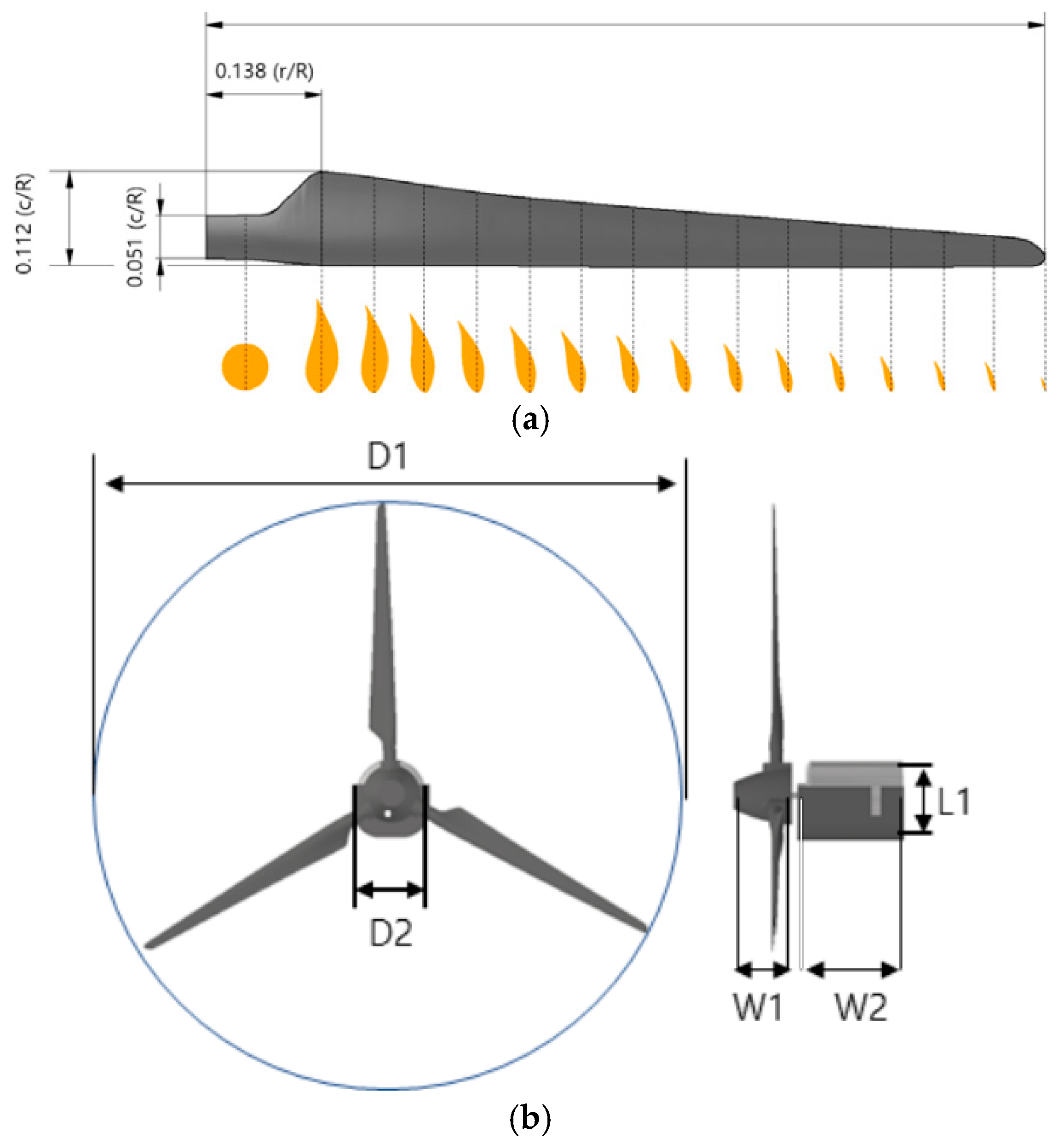
Geometry of scaled 20 kW wind turbine model: (a) Blade normalized to radius (R: Blade length, c: Chord length); (b) Normalized of wind blade size (D: Diameter, L: Nacelle height, W1: Rotor length, W2: Nacelle length).
Figure 2.
Geometry of scaled 20 kW wind turbine model: (a) Blade normalized to radius (R: Blade length, c: Chord length); (b) Normalized of wind blade size (D: Diameter, L: Nacelle height, W1: Rotor length, W2: Nacelle length).
Figure 3.
20 kW wind turbine scale model. (a) 1:33 scale; (b) 1:50 scale; (c) 1:67 scale.
Figure 3.
20 kW wind turbine scale model. (a) 1:33 scale; (b) 1:50 scale; (c) 1:67 scale.
Figure 4.
Experimental setup of scaled wind turbine model in the wind tunnel.
Figure 4.
Experimental setup of scaled wind turbine model in the wind tunnel.
Figure 5.
Measurement points: (a) x-z plane; (b) x-y plane.
Figure 5.
Measurement points: (a) x-z plane; (b) x-y plane.
Figure 6.
Three-dimensional visualization of measurement section in wind tunnel. (a) 1:33 scale model; (b) 1:50 scale model; (c) 1:67 scale model.
Figure 6.
Three-dimensional visualization of measurement section in wind tunnel. (a) 1:33 scale model; (b) 1:50 scale model; (c) 1:67 scale model.
Figure 7.
Normalized horizontally and vertically wake of 1:33 scale model: (a) x-z plane; (b) x-y plane.
Figure 7.
Normalized horizontally and vertically wake of 1:33 scale model: (a) x-z plane; (b) x-y plane.
Figure 8.
Normalized horizontally and vertically wake of 1:50 scale model: (a) x-z plane; (b) x-y plane.
Figure 8.
Normalized horizontally and vertically wake of 1:50 scale model: (a) x-z plane; (b) x-y plane.
Figure 9.
Normalized horizontally and vertically wake of 1:67 scale model: (a) x-z plane; (b) x-y plane.
Figure 9.
Normalized horizontally and vertically wake of 1:67 scale model: (a) x-z plane; (b) x-y plane.
Figure 10.
Normalized horizontally and vertically wake according to normalized separation distance: (a) x-z plane; (b) x-y plane.
Figure 10.
Normalized horizontally and vertically wake according to normalized separation distance: (a) x-z plane; (b) x-y plane.
Figure 11.
Geometry of NREL 5 MW reference wind turbine, front view (
left) and side view (
right) [
20].
Figure 11.
Geometry of NREL 5 MW reference wind turbine, front view (
left) and side view (
right) [
20].
Figure 12.
Boundary conditions and domain size for NREL 5 MW wind turbine numerical simulation [
18].
Figure 12.
Boundary conditions and domain size for NREL 5 MW wind turbine numerical simulation [
18].
Figure 13.
Blade section of NREL 5 MW wind turbine.
Figure 13.
Blade section of NREL 5 MW wind turbine.
Figure 14.
Grid resolution variations on blade surfaces: (a) coarse; (b) medium; (c) fine.
Figure 14.
Grid resolution variations on blade surfaces: (a) coarse; (b) medium; (c) fine.
Figure 15.
Grid geometry according to y+ values: (a) y+1; (b) y+30; (c) y+100.
Figure 15.
Grid geometry according to y+ values: (a) y+1; (b) y+30; (c) y+100.
Figure 16.
y+ scalar for blade surface (scalar range: 0.5 y+ < 1.5 y+): (a) y+1; (b) y+30; (c) y+100.
Figure 16.
y+ scalar for blade surface (scalar range: 0.5 y+ < 1.5 y+): (a) y+1; (b) y+30; (c) y+100.
Figure 17.
Q-criterion 0.01/s2 wind speed contours per blade y+ (Front view): (a) y+1; (b) y+30; (c) y+100.
Figure 17.
Q-criterion 0.01/s2 wind speed contours per blade y+ (Front view): (a) y+1; (b) y+30; (c) y+100.
Figure 18.
Q-criterion difference between y+1 and y+100: (a) y+1; (b) y+100.
Figure 18.
Q-criterion difference between y+1 and y+100: (a) y+1; (b) y+100.
Figure 19.
The time-thrust curve of the NREL 5 MW wind turbine according to y+.
Figure 19.
The time-thrust curve of the NREL 5 MW wind turbine according to y+.
Figure 20.
Grid configurations used for the grid system convergence test: (a) coarse grid on blade tip area—fine grid on inner area; (b) fine grid on blade tip area—coarse grid on inner area; (c) coarse grid on blade tip area with subdivision—fine grid on inner area with subdivision; (d) fine grid on blade tip area with subdivision—coarse grid on inner area with subdivision.
Figure 21.
Visualization of the wake results from the analysis based on grid configuration (front view): (a) coarse grid on blade tip area—fine grid on inner area; (b) fine grid on blade tip area—coarse grid on inner area; (c) coarse grid on blade tip area with subdivision—fine grid on inner area with subdivision; (d) fine grid on blade tip area with subdivision—coarse grid on inner area with subdivision.
Figure 22.
Visualization of the wake results from the analysis based on grid configuration (side view): (a) coarse grid on blade tip area—fine grid on inner area; (b) fine grid on blade tip area—coarse grid on inner area; (c) coarse grid on blade tip area with subdivision—fine grid on inner area with subdivision; (d) fine grid on blade tip area with subdivision—coarse grid on inner area with subdivision.
Figure 23.
Grid configurations used for the 20 kW scale model verification: (a) coarse grid on blade tip area with subdivision—fine grid on inner area with subdivision; (b) fine grid on blade tip area with subdivision—coarse grid on inner area with subdivision.
Figure 23.
Grid configurations used for the 20 kW scale model verification: (a) coarse grid on blade tip area with subdivision—fine grid on inner area with subdivision; (b) fine grid on blade tip area with subdivision—coarse grid on inner area with subdivision.
Figure 24.
Visualization of the wake results from the 20 kW scale model verification analysis based on grid configuration (side view): (a) coarse grid on blade tip area with subdivision—fine grid on inner area with subdivision; (b) fine grid on blade tip area with subdivision—coarse grid on inner area with subdivision.
Figure 25.
Grid configurations of the scaled-down 20 kW wind turbine models: (a) 1:33 scale model; (b) 1:50 scale model; (c) 1:67 scale model.
Figure 25.
Grid configurations of the scaled-down 20 kW wind turbine models: (a) 1:33 scale model; (b) 1:50 scale model; (c) 1:67 scale model.
Figure 26.
Wake velocity profiles according to scale-down ratio (side view): (a) 1:33 scale; (b) 1:50 scale; (c) 1:67 scale.
Figure 26.
Wake velocity profiles according to scale-down ratio (side view): (a) 1:33 scale; (b) 1:50 scale; (c) 1:67 scale.
Figure 27.
Wake velocity profiles according to scale-down ratio (top view): (a) 1:33 scale; (b) 1:50 scale; (c) 1:67 scale.
Figure 27.
Wake velocity profiles according to scale-down ratio (top view): (a) 1:33 scale; (b) 1:50 scale; (c) 1:67 scale.
Figure 28.
Wake velocity profiles according to separation distance (side view): (a) 1D; (b) 2D; (c) 3D; (d) 4D; (e) 5D; (f) 6D; (g) 7D; (h) 8D.
Figure 28.
Wake velocity profiles according to separation distance (side view): (a) 1D; (b) 2D; (c) 3D; (d) 4D; (e) 5D; (f) 6D; (g) 7D; (h) 8D.
Figure 29.
Wake velocity profiles according to separation distance (top view): (a) 1D; (b) 2D; (c) 3D; (d) 4D; (e) 5D; (f) 6D; (g) 7D; (h) 8D.
Figure 29.
Wake velocity profiles according to separation distance (top view): (a) 1D; (b) 2D; (c) 3D; (d) 4D; (e) 5D; (f) 6D; (g) 7D; (h) 8D.
Figure 30.
Wake comparison of experimental and numerical simulation results according separation distance (side view): (a) 1:33 scale model; (b) 1:50 scale model; (c) 1:67 scale model; (line: simulation, square: experiments).
Figure 30.
Wake comparison of experimental and numerical simulation results according separation distance (side view): (a) 1:33 scale model; (b) 1:50 scale model; (c) 1:67 scale model; (line: simulation, square: experiments).
Figure 31.
Wake comparison of experimental and numerical simulation results according to separation distance (top view): (a) 1:33 scale model; (b) 1:50 scale model; (c) 1:67 scale model; (line: simulation, square: experiments).
Figure 31.
Wake comparison of experimental and numerical simulation results according to separation distance (top view): (a) 1:33 scale model; (b) 1:50 scale model; (c) 1:67 scale model; (line: simulation, square: experiments).
Figure 32.
Error rate according to separation distance (side view): (a) 1:33 scale model; (b) 1:50 scale model; (c) 1:67 scale model (line: simulation, square: experiments).
Figure 32.
Error rate according to separation distance (side view): (a) 1:33 scale model; (b) 1:50 scale model; (c) 1:67 scale model (line: simulation, square: experiments).
Figure 33.
Error rate according to separation distance (top view): (a) 1:33 scale model; (b) 1:50 scale model; (c) 1:67 scale model (line: simulation, square: experiments).
Figure 33.
Error rate according to separation distance (top view): (a) 1:33 scale model; (b) 1:50 scale model; (c) 1:67 scale model (line: simulation, square: experiments).
Figure 34.
Non-dimensional experimental velocity magnitudes at the lateral position Z/D = +0.5 in relation to the separation distance for each scale model.
Figure 34.
Non-dimensional experimental velocity magnitudes at the lateral position Z/D = +0.5 in relation to the separation distance for each scale model.
Figure 35.
Non-dimensional numerical simulation velocity magnitudes at the lateral position Z/D = +0.5 in relation to the separation distance for each scale model.
Figure 35.
Non-dimensional numerical simulation velocity magnitudes at the lateral position Z/D = +0.5 in relation to the separation distance for each scale model.
Table 1.
Normalized wind turbine blade and shape size.
Table 1.
Normalized wind turbine blade and shape size.
| Category (Symbol) | Scale (-) | 1:33 (m) | 1:50 (m) | 1:67 (m) |
|---|
| Main blade diameter (D1) | 1.0D | 0.3 | 0.2 | 0.15 |
| Rotor diameter (D2) | - | 0.04 | 0.026 | 0.026 |
| Nacelle height (L1) | 0.13D | 0.04 | 0.026 | 0.02 |
| Rotor length (W1) | 0.10D | 0.03 | 0.02 | 0.015 |
| Nacelle length (W2) | 0.18D | 0.055 | 0.036 | 0.027 |
| Blockage ratio | - | 4.9% | 2.2% | 1.2% |
Table 2.
Thrust values for the NREL 5 MW wind turbine based on blade surface grid resolution.
Table 2.
Thrust values for the NREL 5 MW wind turbine based on blade surface grid resolution.
| Grid Resolution | Total Number of Elements in Rotor Region | Average Thrust (kN) | Error Rate (%) |
|---|
| Coarse | 1.65 × 10⁶ | 713.2 | 4.01 |
| Medium | 3.13 × 10⁶ | 730.6 | 1.67 |
| Fine | 6.94 × 10⁶ | 740.9 | 0.28 |
Table 3.
The thrust table of the NREL 5 MW wind turbine according to y+ (Range: 132.1902 s~133.8876 s).
Table 3.
The thrust table of the NREL 5 MW wind turbine according to y+ (Range: 132.1902 s~133.8876 s).
| Y+ Value | Total Number of Elements in Rotor Region | Range (kN) | Average (kN) | Error Rate (%) |
|---|
| Min. | Max. |
|---|
| Y+ 1 | 4.81 × 10⁶ | 729.9 | 748.1 | 743.4 | 0.05 |
| Y+ 30 | 3.13 × 10⁶ | 719.4 | 735.4 | 730.6 | 1.67 |
| Y+ 100 | 2.37 × 10⁶ | 721.2 | 737.4 | 732.9 | 1.36 |
Table 4.
Numerical setup for the simulation of scaled-down wind turbine models.
Table 4.
Numerical setup for the simulation of scaled-down wind turbine models.
| Scale (Units) | 1:33 (m) | 1:50 (m) | 1:67 (m) |
|---|
| Rotor diameter (mm) | 300 | 200 | 150 |
| Inflow wind (m/s) | 6.7 |
| RPM | 2431.3 | 3647.9 | 4862.5 |
| Time step (s) | 1.03 × 10⁻³ | 6.85 × 10⁻⁴ | 5.14 × 10⁴ |
| Total mesh (-) | 143.5 × 10⁶ | 153.6 × 10⁶ | 169.4 × 10⁶ |
| Measurement section | 1D–4D | 1D–6D | 1D–8D |
Table 5.
Experimental data (EXP) for 1:33 scale at various measure points.
Table 5.
Experimental data (EXP) for 1:33 scale at various measure points.
| Measure Point | 1D | 2D | 3D | 4D |
|---|
| 0.0D | 0.6871 | 0.7309 | 0.7561 | 0.7752 |
| Side | 0.5D | 0.9552 | 0.9570 | 0.9486 | 0.9443 |
| 1.0D | 1.0114 | 1.0124 | 1.0091 | 1.0155 |
| Top | 0.5D | 0.9959 | 0.9873 | 0.9896 | 0.9910 |
| 1.0D | 1.013 | 1.010 | 1.011 | 1.017 |
Table 6.
Computational Fluid Dynamics (CFD) for 1:33 scale at various measure points.
Table 6.
Computational Fluid Dynamics (CFD) for 1:33 scale at various measure points.
| Measure Point | 1D | 2D | 3D | 4D |
|---|
| 0.0D | 0.5144 | 0.6564 | 0.6247 | 0.6657 |
| Side | 0.5D | 0.9627 | 0.9724 | 0.9906 | 0.9868 |
| 1.0D | 1.0284 | 1.0295 | 1.0309 | 1.0328 |
| Top | 0.5D | 0.9824 | 0.9853 | 0.9929 | 1.0026 |
| 1.0D | 1.0270 | 1.0290 | 1.0300 | 1.0320 |
Table 7.
Experimental data (EXP) for 1:50 scale at various measure points.
Table 7.
Experimental data (EXP) for 1:50 scale at various measure points.
| Measure Point | 1D | 2D | 3D | 4D | 5D | 6D |
|---|
| 0.0D | 0.7132 | 0.7597 | 0.7752 | 0.7907 | 0.8217 | 0.8527 |
| Side | 0.5D | 0.9740 | 0.9527 | 0.9509 | 0.9496 | 0.9483 | 0.9576 |
| 1.0D | 1.0120 | 1.0089 | 1.0066 | 1.0036 | 1.0094 | 1.0115 |
| Top | 0.5D | 0.9384 | 0.9378 | 0.9409 | 0.9345 | 0.9417 | 0.9374 |
| 1.0D | 1.0158 | 1.0144 | 1.0166 | 1.0103 | 1.0107 | 1.0111 |
Table 8.
Computational Fluid Dynamics (CFD) for 1:50 scale at various measure points.
Table 8.
Computational Fluid Dynamics (CFD) for 1:50 scale at various measure points.
| Measure Point | 1D | 2D | 3D | 4D | 5D | 6D |
|---|
| 0.0D | 0.6982 | 0.6885 | 0.7043 | 0.7415 | 0.7629 | 0.7726 |
| Side | 0.5D | 0.9765 | 0.9799 | 0.9822 | 0.9920 | 0.9972 | 1.0025 |
| 1.0D | 1.0239 | 1.0231 | 1.0233 | 1.0241 | 1.0252 | 1.0266 |
| Top | 0.5D | 0.9769 | 0.9946 | 1.0004 | 1.0055 | 1.0081 | 1.0126 |
| 1.0D | 1.0240 | 1.0236 | 1.0235 | 1.0242 | 1.0253 | 1.0264 |
Table 9.
Experimental data (EXP) for 1:67 scale at various measure points.
Table 9.
Experimental data (EXP) for 1:67 scale at various measure points.
| Measure Point | 1D | 2D | 3D | 4D | 5D | 6D | 7D | 8D |
|---|
| 0.0D | 0.7369 | 0.7590 | 0.8086 | 0.8385 | 0.8539 | 0.8976 | 0.8935 | 0.9213 |
| Side | 0.5D | 1.0089 | 0.9574 | 1.0003 | 0.9989 | 0.9721 | 0.9916 | 0.9780 | 1.0019 |
| 1.0D | 1.0078 | 0.9979 | 0.9946 | 0.9959 | 0.9782 | 0.9969 | 0.9914 | 0.9940 |
| Top | 0.5D | 0.9728 | 0.9729 | 0.9946 | 0.9976 | 0.9884 | 0.9995 | 0.9841 | 0.9958 |
| 1.0D | 0.9989 | 0.9983 | 0.9981 | 1.0121 | 1.0033 | 1.0297 | 1.0088 | 1.0255 |
Table 10.
Computational Fluid Dynamics (CFD) for 1:67 scale at various measure points.
Table 10.
Computational Fluid Dynamics (CFD) for 1:67 scale at various measure points.
| Measure Point | 1D | 2D | 3D | 4D | 5D | 6D | 7D | 8D |
|---|
| 0.0D | 0.7649 | 0.7007 | 0.6951 | 0.7324 | 0.7678 | 0.7867 | 0.8020 | 0.8068 |
| Side | 0.5D | 0.9675 | 0.9694 | 0.9791 | 0.9862 | 0.9926 | 0.9961 | 1.0005 | 1.0028 |
| 1.0D | 1.0204 | 1.0194 | 1.0192 | 1.0196 | 1.0204 | 1.0212 | 1.0222 | 1.0231 |
| Top | 0.5D | 0.9667 | 0.9810 | 0.9911 | 0.9906 | 0.9993 | 0.9973 | 1.0040 | 1.0057 |
| 1.0D | 1.0208 | 1.0200 | 1.0196 | 1.0198 | 1.0204 | 1.0212 | 1.0221 | 1.0231 |
Table 11.
Error rate comparison at 0.5D position according to scale ratio.
Table 11.
Error rate comparison at 0.5D position according to scale ratio.
| Scale | 1:33 Scale | 1:50 Scale | 1:67 Scale | MU
(%) |
|---|
| X/D | Side | Top | Side | Top | Side | Top |
|---|
| 1 | 0.8 | 1.8 | 0.3 | 4.2 | 4.1 | 0.9 | 3.54 |
| 2 | 1.6 | 2.4 | 2.9 | 6.1 | 1.2 | 2.0 |
| 3 | 4.4 | 2.9 | 3.3 | 6.4 | 2.1 | 1.9 |
| 4 | 4.5 | 3.3 | 4.5 | 7.7 | 1.3 | 2.3 |
| 5 | - | - | 5.2 | 7.1 | 2.1 | 1.8 |
| 6 | - | - | 4.7 | 8.0 | 0.5 | 2.5 |
| 7 | - | - | - | - | 2.3 | 2.1 |
| 8 | - | - | - | - | 0.1 | 1.4 |
Table 12.
Error rate comparison at 1.0D position according to scale ratio.
Table 12.
Error rate comparison at 1.0D position according to scale ratio.
| Scale | 1:33 Scale | 1:50 Scale | 1:67 Scale | MU
(%) |
|---|
| X/D | Side | Top | Side | Top | Side | Top |
|---|
| 1 | 1.7 | 1.5 | 1.2 | 2.1 | 1.3 | 2.2 | 3.54 |
| 2 | 1.7 | 1.9 | 1.4 | 2.4 | 2.2 | 2.2 |
| 3 | 2.2 | 1.8 | 1.7 | 2.4 | 2.5 | 2.2 |
| 4 | 1.7 | 1.5 | 2.0 | 2.3 | 2.4 | 1.2 |
| 5 | - | - | 1.6 | 2.0 | 4.3 | 1.7 |
| 6 | - | - | 1.5 | 1.9 | 2.4 | 0.8 |
| 7 | - | - | - | - | 3.1 | 1.3 |
| 8 | - | - | - | - | 2.9 | 0.7 |


