A Comparative Study of Data-Driven Early-Stage End-of-Life Classification Approaches for Lithium-Ion Batteries

Abstract

Lithium-ion batteries are the most widely used as energy storage devices in electric mobility applications. However, due to complex electrochemical processes of battery degradation, it is challenging to predict accurately the battery end-of-life (EOL) to ensure their reliability, safety, and extended usage. In this context, the introduction of machine learning techniques can provide relevant solutions based on data collection and analysis. Indeed, we compared in this study the prediction performance of numerous machine learning approaches that predict if the battery EOL bypasses a predefined threshold. Based on the variation of different indicators during the first several hundred cycles, such as charge and discharge capacity, internal resistance, and energy efficiency, extensive numerical tests have been executed and compared in terms of accuracy score, precision score, recall score, etc. All the studied machine learning approaches are trained and validated using an open-access database of 124 commercial lithium iron phosphate/graphite cells cycled under different fast-charging conditions. As a result, the classification prediction performance score reached up to 98.74% depending on the percentage of data and cycles used for training and validation as well as the predefined EOL threshold. The comparative results can be used to improve the existing health-aware energy management strategy by taking the state-of-health (SOH) of batteries into consideration. Overall, the presented research findings are relevant to battery system reliability and safety engineering.

1. Introduction

Lithium-ion batteries (LIB) are widely used as an energy storage system, playing an important role in a diverse domain of industry [1]. Particularly in the automobile industry, LIB is the main energy storage device for electric mobility applications due to its energy density, production cost, and stability [2,3,4].

One of the paramount challenges facing the widespread adoption of LIB is the accurate prediction of their state-of-health (SOH) and remaining useful life (RUL). Due to the chemical degradation of LIB, its electrical performance decreases as cycle life increases during daily usage [1,5]. Battery degradation leads to not only a lower performance but also the increase of battery security issues such as thermal runaway caused by short circuit, which is one of the main concerns regarding electric vehicles security and stability [6,7]. Being able to accurately estimate when a battery will reach the end of its operational life is not only crucial for optimizing energy storage systems but also has significant influence on cost-effectiveness, sustainability, and safety [8,9,10]. In many applications, such as electric vehicles, unexpected battery failures can result in not only financial losses but also threaten user safety and public trust in emerging technologies. As a result, predicting the RUL and SOH of LIB raises the interests of researchers [1,11,12].

Traditional methods for RUL prediction often rely on empirical aging models or simplistic rule-based approaches, which may not fully capture the intricacies of battery degradation (Figure 1) [13]. These conventional techniques are inferior due to their limited adaptability to diverse operating conditions and the ever-evolving landscape of battery chemistry and designs. As a result, there is a growing imperative to explore innovative data-driven methodologies by using machine learning, such as fast pulse tests using random forest [14] and federated machine-learning-based diagnostics platforms [15] to enhance the precision and flexibility of battery RUL predictions [16].

The primary objective of this study is to efficiently classify the lifespan potential of lithium-ion batteries, determining whether a battery is likely to exceed a specific cycle life threshold without necessitating precise predictions of its RUL. The classification approach is particularly valuable in various contexts where rapid and reliable assessments of battery longevity are crucial for optimizing performance and maintenance strategies. This study aims to identify the most effective algorithms for this task by employing machine learning classification methods and offer a practical solution that balances accuracy with computational efficiency. These methods not only streamline the prediction process but also facilitate the prioritization of batteries for further online monitoring or replacement based on their estimated lifecycle category, thereby enabling more informed and proactive management of battery assets in multiple application scenarios such as online SOH estimation and diagnostics of BMS for new energy vehicles (NEV). Figure 2 shows a general framework of a BMS. Having access to the results of RUL estimation by using machine learning classification helps to improve the decision-making strategy for the SOH estimation module in the system [17].

In this article, several machine learning methods are used to predict the RUL. A LIB aging database, consisting of 124 cells and realized by Severson et al., [18], is reused, and a classification model is established to predict whether the end-of-life (EOL) of each cell surpasses a certain threshold. The research utilizes a comprehensive database of 124 commercial lithium iron phosphate/graphite cells subjected to various fast-charging conditions. Focusing specifically on cells with a cycle life ranging from 400 to 2300 cycles, the study ensures that our analysis encompassed a representative sample of battery behavior over time. Our machine learning models were trained and validated using this database. We achieved a significant result of prediction accuracy ranging from 60% to 90%. Such variation in accuracy depends on factors such as the percentage of data used for training and validation and the predefined EOL threshold. Incorporating SOH considerations into the models has the potential to significantly enhance the longevity and durability of LIB, therefore extending their useful life and improving the reliability of electric vehicles and other applications [19].

This article delves into the field of data-driven RUL estimation for LIB, aiming to address the inherent challenges posed by battery degradation processes. By comparing the prediction accuracy of various machine learning models and leveraging a rich dataset from commercial lithium iron phosphate/graphite cells, valuable insights and methodologies are contributed. These findings have the potential to advance the understanding of LIB behavior and empower the optimization of energy management and battery management strategies. Ultimately, the goal is to bolster the longevity and sustainability of LIB, thereby enhancing their role in the electrification of the automotive industry and supporting the transition towards more reliable and efficient energy management practices.

The structure of this article is methodically organized as follows: Section 2 provides a comprehensive explanation of the primary degradation mechanism of lithium-ion batteries. Section 3 delineates the methodology, presenting the database utilized for model training and detailing the 11 classification models alongside the evaluation scores employed to judge their performance. Section 4 offers a comprehensive exposition of the results, wherein the performance scores of each model are analyzed across differing scenarios. Section 5 provides a discussion with comparative analysis and particularly recommendations for improving performance in our future work. Concluding the article, Section 6 synthesizes our findings and provides critical reflections, encapsulating the essence and implications of the research outcomes. Additionally, Figure 3 represents the general process of methodology in this research.

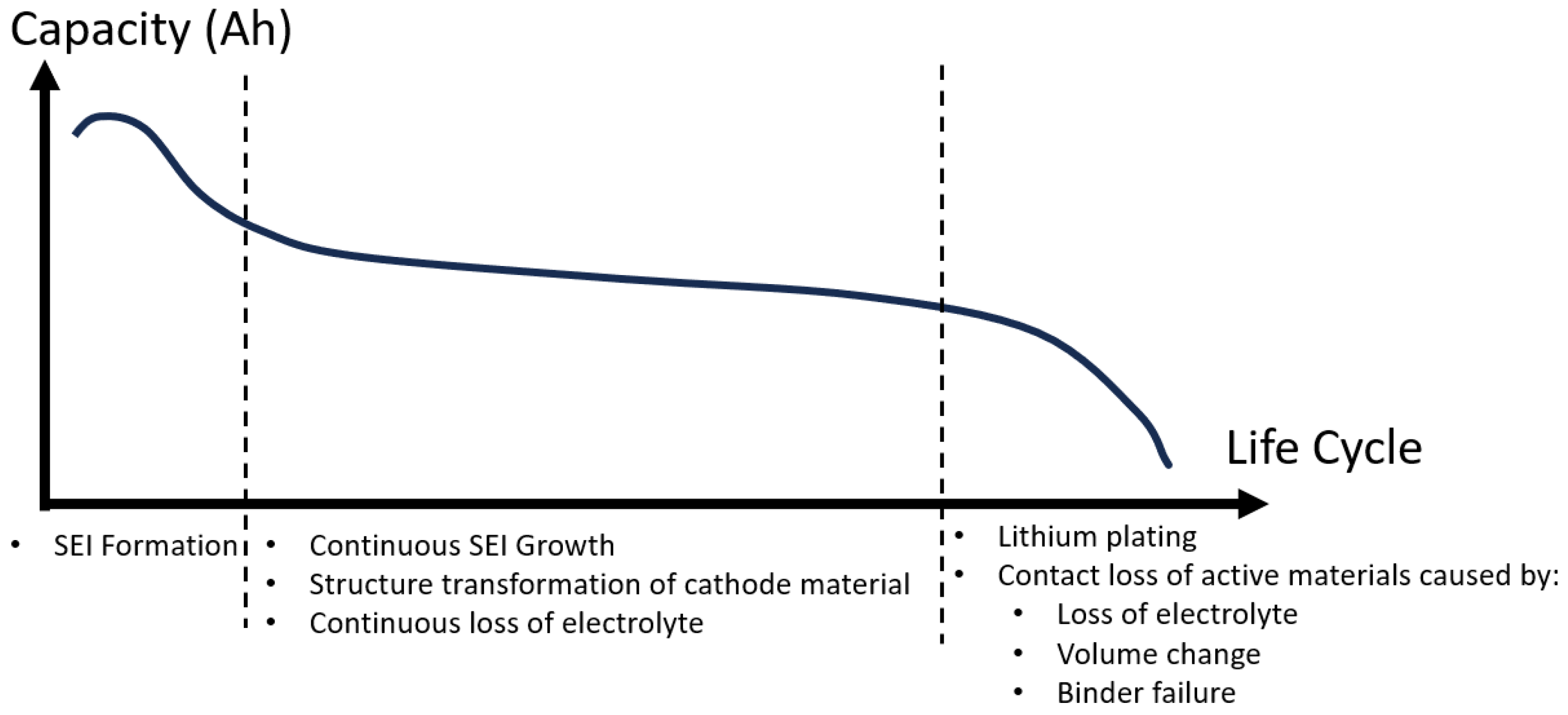
2. Chemical Mechanism for Li-Ion Battery Primary Degradation

LIB degradation involves a series of complex electrochemical reactions. These electrochemical reactions can be classified into three types by different effects of degradation, namely: loss of lithium inventory, loss of active delithiated anode material, and loss of active cathode material. Different chemical models are established to simulate the process of degradation, but those microscale processes are not easy to precisely simulate. The main degradation is resumed as follows [6,20,21,22] and illustrated in Figure 4:

2.1. Loss of Lithium Inventory (LLI)

Lithium ions are consumed by parasitic reactions, such as surface film formation (e.g., solid electrolyte interphase (SEI) growth), decomposition reactions, and lithium plating [22]. These ions are no longer available for cycling between the positive and negative electrodes, which leads to a battery capacity fade. Additionally, surface films can contribute to a reduction in power output. Lithium ions may also become unavailable if they are trapped within electrically isolated particles of the active materials [24].

2.2. Loss of Active Material of the Negative Electrode (LAM_NE)

The active material of the negative electrode (or anode) becomes unavailable for lithium insertion due to factors like particle cracking, loss of electrical contact, or the blockage of active sites by resistive surface layers. These issues can result in both a decline in battery capacity and a reduction in power output [22,24,25].

2.3. Loss of Active Material of the Positive Electrode (LAM_PE)

The active material of the positive electrode (or cathode) becomes unavailable for lithium insertion due to structural disordering, particle cracking, or the loss of electrical contact. For example, Jia et al. mentioned that the failure of LiFePO4 (LFP) cathodes in lithium-ion batteries primarily stems from the migration of iron (Fe) ions within the material’s structure, leading to irreversible phase transitions and reduced lithium-ion diffusion [26]. These processes can lead to both a reduction in battery capacity and a decrease in power output [22,24,25].

These LIB degradation mechanisms lead to changes on the electrical profile of each cell as a typical phenomenon caused by battery aging mechanisms. Figure 5 illustrates the profile of capacity fade and possible mechanisms [6,27].

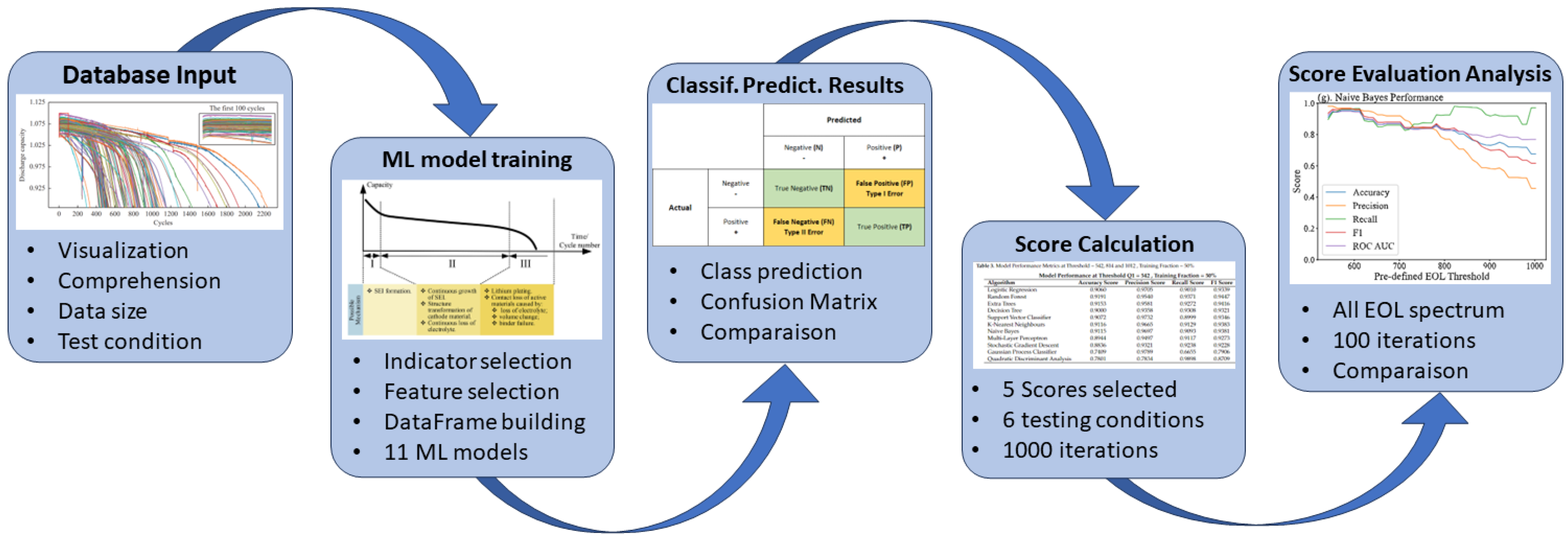
3. Methodology for Battery EOL Classification Estimation

The main objective is to develop a classification model capable of predicting whether the EOL of LIB will exceed a predefined threshold. Generally, our methodology integrates several key components to construct a robust classification model for LIB EOL prediction. Firstly, a comprehensive database providing a rich source of battery performance data is utilized to train our machine learning classification algorithms. A set of pertinent features is selected from this database, focusing on those associated with changes in charge/discharge capacity, energy, and energy efficiency. Subsequently, each dataset is then labeled according to a specific EOL threshold, effectively distinguishing cells that exceed this threshold from those that do not, simplifying the process for more accurate prediction outcomes.

3.1. Selected Database for Classification Training

The used database is provided by Severson et al. [18], which contains the degradation variation data of 124 commercial lithium iron phosphate/graphite cells (A123 Systems, model APR18650M1A, 1.1 Ah nominal capacity). The charging rate varies from the manufacturer’s recommended fast-charging rate of 3.6 C constant current–constant voltage (CC-CV) to 6 C, probing the performance of current-generation power cells under extreme fast-charging conditions (about 10 min charging), as is shown in

Table 1. APR18650M1B Battery Specifications.

Parameter	Specification
Nominal capacity and voltage	1.1 Ah, 3.3 V
Recommended standard charge method	1.5 A to 3.6 V CC-CV, 45 min
Recommended fast charge current	4 A to 3.6 V CC-CV, 15 min
Maximum continuous discharge	30 A
Recommended charge and cut-off V at 25 °C	3.6 A to 2 V
Operating temperature range	−30 °C to +60 °C
Storage temperature range	−50 °C to +60 °C
Core cell weight	39 g

. By varying the charging conditions, a database that captures a wide range of cycle lives, from approximately 150 to 2300 cycles (average cycle life of 806 with a standard deviation of 377) is generated [18].

These cells were cycled in an isotherm chamber set to 30 °C under different fast-charging conditions and identical discharging rate (4 C to 2.0 V, where 1 C is 1.1 A). The cell temperatures vary by less than 10 °C due to the heat generated during the charging and discharging process inside the isotherm chamber within a cycle. All cells in this database are charged using a two-step fast-charging policy. This protocol follows the format “C1(Q1)-C2,” where C1 and C2 represent the first and second constant-current steps, respectively, and Q1 indicates the state-of-charge (SOC, %) at which the current changes to C2. The second current step continues until the SOC reaches 80%, after which the cells charge at 1C using a CC-CV method. The upper and lower cutoff voltages are in accordance with the manufacturer’s specifications of 3.6 V and 2.0 V, respectively. These cutoff voltages remain constant for all current steps, including during fast charging. After a number of charge cycles, the cells may reach the upper cutoff voltage during fast charging, resulting in extended constant-voltage charging. Figure 6 represents an example of charging/discharge cycle with a protocol of 5.2 C(66%)–3.5 C ($\mathrm{C}1=5.2$, $\mathrm{Q}1=66\%$, and $\mathrm{C}2=3.5$). The cell is charged to 66% of SOC in 5.5 C and then in 3.5 C to 80% [18].

3.2. Feature Selection

The data for our analysis were systematically organized in a structured format, with each unit of data corresponding to individual battery cell performance over its life cycle. The analysis and training of our machine learning models were conducted using aggregated summaries of these cycles, emphasizing the critical features that demonstrate the battery’s performance variation throughout its operational life. The used indicators are given as follow:

• Cycle index: This feature indicates the real-life cycle count of each cell, serving as the benchmark for our classification algorithm’s threshold.
• Charged/discharged capacity: Capacity fade is a critical occurrence that results from the loss of lithium inventory and the loss of active anode material, which are primary degradation modes triggered by various chemical reactions causing battery aging as presented in Figure 7a,b.
• Charged/discharged energy and energy efficiency: During charge-discharge cycles in a degraded battery, the increased internal resistance causes more energy to be lost as heat. This inefficiency means less energy is stored during charging and less is available for use during discharging, leading to overall energy loss as presented in Figure 7c,d.
• Average/maximum/minimun temperature: Due to increased internal resistance and breakdown of internal components, inefficient current flow leads to excess heat generation during operation, which manifests as temperature fluctuations as presented in Figure 7e.
• DC internal resistance: Battery degradation leads to an increase in DC internal resistance primarily due to the formation of internal chemical byproducts and the loss of electrode materials. Over time, these processes hinder the efficient flow of ions within the battery, thereby increasing its internal resistance as presented in Figure 7f.

3.3. Data Pre-Treatment

The selection of pertinent features is a critical aspect of our research to enhance the performance and efficiency classification prediction of EOL. Emphasis has been placed on examining features related to charge/discharge capacity, energy, DC internal resistance, and energy efficiency due to their direct relevance to battery health assessment. These features exhibit a notably reduced level of noise in their variations, providing the robustness for predictive models. Moreover, their trends of gradual decreasing tendency throughout the battery’s life cycle are markedly clear and consistent: Charge/discharge capacity and energy decrease directly reflect the shrinkage in storing and delivering energy. Energy efficiency decrease, in turn, quantifies the effectiveness drop of energy conversion processes, which makes it also a critical factor in understanding battery degradation. The augmentation of internal resistance further indicates the drop of energy conversion processes due to side reactions.

To precisely capture the nuances of variation within each indicator and thereby enhance the processing capabilities of classification models, a selection of parameters has been identified to describe the variation of each indicator effectively, as described in

Table 2. Definition of each parameter used to describe the variation profile.

Parameter	Definition
$X_0$	Initial value of cycle 0
$X_{400}$	Value at cycle 400
$(X_{(400-\alpha )}-X_{400})/\alpha$	Derivative between cycle 400 − $\alpha$ and 400
$(X_{(400-2\alpha )}-X_{400})/2\alpha$	Derivative between cycle 400 − 2$\alpha$ and 400
	(with $\alpha$ the selected interval, $\alpha =100$ in the following sections)
$X_{i_{max}}$, $i_{max}$	Maximal value and its cycle index

.

3.4. Data-Driven Approach for EOL Classification

The selection of machine learning models in this study was driven by the need to balance predictive accuracy, computational efficiency, and model interpretability. We chose a diverse set of models ranging from simple linear models to more complex models to capture non-linear relationships and complex interactions between features.

Logistic regression was selected as a baseline model due to its simplicity and interpretability, making it a useful tool for understanding the fundamental relationships in the data. However, because battery degradation often involves complex, non-linear processes, ensemble methods like Random Forest and Extra Trees were also included. These models are particularly suited to handling high-dimensional data and capturing the intricate patterns that may not be apparent in simpler models.

In addition, support vector classifiers were selected for their ability to find optimal hyperplanes in feature space, which is critical for making precise distinctions between classes in a binary classification problem like EOL prediction. K-Nearest Neighbors and tree structure models were included to explore the trade-offs between simplicity, computational cost, and accuracy.

Furthermore, we included neural network-based models like multi-layer perceptron, which are capable of modeling more complex, non-linear relationships in the data. However, recognizing that these models require significant computational resources and may suffer from overfitting, we also compared them against models like Gaussian process classifiers and quadratic discriminant analysis, which offer probabilistic predictions and can model non-linear decision boundaries with more theoretical rigor.

• Logistic regression: This model is opted as a baseline model due to its simplicity, transparency, and interpretability. As a linear model, it provides a clear understanding of how individual features contribute to the probability of EOL prediction. While logistic regression may be considered less complex compared to other models, it serves as a valuable benchmark to assess the performance of more complex algorithms [28,29].
• Random forest classifier: The random forest classifier was selected because it can handle non-linearity, complex interactions between features, and resistance to overfitting. Intricate degradation patterns that may not be evident in simpler models can thus be captured. This model’s ensemble approach offers robustness and the potential to achieve high predictive accuracy [30].
• Extra tree classifier: Similar to the random forest classifier, the extra tree classifier was selected due to its ensemble nature, which mitigates overfitting and captures subtle variations in data. It was chosen to assess whether it provides a significant improvement over the Random Forest model, given its distinct tree-building strategy [31].
• Decision tree classifier: The decision tree classifier was introduced due to the simplicity and ability to partition the feature space into easily interpretable decision rules. Despite being susceptible to overfitting, the decision tree classifier is included as a comparative reference to measure the trade-off between interpretability and model performance [32].
• Support vector classifier: Support vector classifier is effective for both binary and multiclass classification. The objective is to find the hyperplane, which separates different classes within a maximized margin [30].
• K-nearest neighbors classifier: The K-nearest neighbors classifier is a non-parametric classifier that assigns labels to data points based on the majority class among the k-nearest neighbors in feature space [31].
• Naive Bayes classifier: The naive Bayes classifier is based on Bayes’ theorem; it employs a probabilistic mechanism, assuming independence among features to simplify the computation of conditional probabilities. This mechanism enables efficient model training and quick prediction generation.
• Multi-layer perceptron (MLP) classifier: This is an artificial neural network with multiple hidden layers; it captures complex relationships in data through its layered structure. However, the complexity can lead to challenges in training, requiring significant computational resources and time.
• Stochastic gradient descent (SGD) classifier: The SGD classifier iteratively updates the model parameters by considering a random subset of the training data, enabling it to efficiently handle large datasets while continuously enhancing the model’s performance [33].
• Gaussian process classifier: A sophisticated machine learning technique that leverages the power of Gaussian processes. It provides a flexible and probabilistic framework for classification tasks, enabling it to model complex relationships and uncertainties in the data. The Gaussian process classifier is particularly suited for scenarios where understanding the confidence of predictions and managing non-linear decision boundaries are crucial.
• Quadratic discriminant analysis: A discriminative modeling approach that captures non-linear decision boundaries by modeling the data point distribution for each class, offering flexibility in classification tasks.

The selection of these models reflects our goal of comparing the predictive capabilities of different algorithms. By employing a diverse set of models, the objective is to evaluate their strengths and weaknesses in the context of LIB EOL prediction, ultimately enabling us to make informed recommendations for practical applications.

3.5. Model Performance Evaluation Score

In the context of classification predictions, the outcomes are quantified as binary variables. Thus, the adoption of a confusion matrix becomes essential for articulating the results. In order to evaluate the predictive accuracy of the models, scores such as accuracy, precision, recall, F1 score, and the area under the receiver operating characteristic curve (AUC ROC) score are systematically applied. These metrics are computed based on the components of the confusion matrix: true positives (TP), true negatives (TN), false positives (FP), and false negatives (FN). It offers a multidimensional perspective on the effectiveness of the predictive models under investigation [34,35,36,37].

• Accuracy: Accuracy score is a straightforward metric that measures the ratio of correctly predicted instances to the total number of instances in the database. The accuracy score can be the most important score to evaluate the performance of a classification model. The expression of accuracy score is:

  $$Accuracy={\displaystyle \frac{TP+TN}{TP+TN+FP+FN}}$$

  (1)
• Precision: Precision measures the ratio of correctly predicted positive instances (TP) to the total number of instances predicted as positive (TP + FP). Precision is useful when minimizing false positives. The expression of precision score is:

  $$Precision={\displaystyle \frac{TP}{TP+FP}}$$

  (2)
• Recall (Sensitivity or True Positive Rate (TPR)): Recall measures the ratio of correctly predicted positive instances (TP) to the total number of actual positive instances (TP + FN). It is useful for the purpose of minimizing false negatives. The expression of recall score is:

  $$Recall={\displaystyle \frac{TP}{TP+FN}}$$

  (3)
• F1-Score: The F1-score is the harmonic mean of precision and recall. It provides a balance between precision and recall. It is useful when an overall measure of a model’s performance is required. The expression of F1-score is:

  $$F1=2\times {\displaystyle \frac{Precision\times Recall}{Precision+Recall}}$$

  (4)
• ROC AUC (Receiver Operating Characteristic—Area Under the Curve): ROC AUC is defined as the area under the receiver operating characteristic curve, which is the plot of the true positive rate (TPR) against the false positive rate (FPR) at each threshold setting. This score evaluates a model’s ability to distinguish between classes across different threshold values. It is particularly useful for imbalanced databases [36].

These scores not only enable us to evaluate the individual performance of each model but also simplify a comparative analysis to identify the most suitable models for predicting battery EOL under varying conditions. This comparative approach allows us to understand the strengths and limitations of each algorithm and make wise decisions during practical application.

4. Results and Analysis

This section presents a sample of preliminary work on the comparative analysis and performance evaluation of different machine learning models of classification. In this context, we conducted a study by varying both the training rate and the EOL threshold. This approach allowed us to explore different scenarios and obtain initial crucial indicators to evaluate the predictive performance of the models. By adjusting the training rate, the performance evolution based on the amount of data used to train each classification model was observed. This variation provided valuable insights into the models’ sensitivity to the size of the training set. Thus, we could determine our models’ ability to generalize from a limited data set or, conversely, to benefit from a large volume of data to enhance their performance. Similarly, an evolution of classification prediction performance was also explored based on a different predefined EOL threshold. The threshold plays a crucial role in the trade-off between precision and recall (sensitivity) of our models. By adjusting this threshold, we analyzed how our models handle FP and FN, essential for understanding their utility in specific applications.

In order to evaluate the performance of each predictive model, several EOL threshold values were strategically selected based on a detailed analysis of the EOL distribution. To determine these thresholds, the spectrum was divided between the minimum and maximum observed EOL values into equal parts. Specifically, three medians were calculated to serve as a central reference point, which were chosen to represent a spread of short, middle, and long lifetime cells. These thresholds are visually marked on the accompanying histogram in Figure 8, which illustrates the frequency distribution of EOL values across the cell population. This histogram highlights the selected median points, thereby contextualizing our threshold selection in relation to the overall EOL data.

4.1. Classification Prediction Results

By defining an EOL threshold of prediction and a certain percentage of training data, we managed to evaluate the classification prediction performance of each machine learning model. In order to ensure reproducibility and robustness, a comprehensive simulation of 1000 predictive iterations was conducted. Each iteration was initialized with a distinct random state seed, thereby randomizing the order of the training dataset and simulating a diverse set of training conditions. Performance scores such as were computed for each individual run.

Table 3. Model Performance Metrics at Threshold = 542, 814 and 1012, Training Fraction = 50%.

Model Performance at Threshold Q1 = 542, Training Fraction = 50%
Algorithm	Accuracy Score	Precision Score	Recall Score	F1 Score	ROC AUC
Logistic Regression	0.9060	0.9705	0.9010	0.9339	0.9114
Random Forest	0.9191	0.9540	0.9371	0.9447	0.9807
Extra Trees	0.9153	0.9581	0.9272	0.9416	0.9782
Decision Tree	0.9000	0.9358	0.9308	0.9321	0.8724
Support Vector Classifier	0.9072	0.9732	0.8999	0.9346	0.9145
K-Nearest Neighbours	0.9116	0.9665	0.9129	0.9383	0.9115
Naive Bayes	0.9115	0.9697	0.9093	0.9381	0.9138
Multi-Layer Perceptron	0.8944	0.9497	0.9117	0.9273	0.8792
Stochastic Gradient Descent	0.8836	0.9321	0.9238	0.9228	0.8487
Gaussian Process Classifier	0.7409	0.9789	0.6655	0.7906	0.8124
Quadratic Discriminant Analysis	0.7801	0.7834	0.9898	0.8709	0.5946
Model Performance at Threshold Q2 = 814, Training Fraction = 50%
Algorithm	Accuracy Score	Precision Score	Recall Score	F1 Score	ROC AUC
Logistic Regression	0.8509	0.8476	0.8614	0.8507	0.8530
Random Forest	0.9501	0.9363	0.9672	0.9504	0.9874
Extra Trees	0.9364	0.9191	0.9589	0.9370	0.9852
Decision Tree	0.9139	0.9186	0.9108	0.9124	0.9161
Support Vector Classifier	0.8314	0.8377	0.8425	0.8308	0.8346
K-Nearest Neighbours	0.9297	0.9385	0.9229	0.9282	0.9306
Naive Bayes	0.8296	0.7559	0.9728	0.8492	0.8308
Multi-Layer Perceptron	0.7633	0.7353	0.8606	0.7732	0.7666
Stochastic Gradient Descent	0.7549	0.7233	0.8231	0.7394	0.7570
Gaussian Process Classifier	0.8191	0.9628	0.6632	0.7823	0.8188
Quadratic Discriminant Analysis	0.7522	0.7542	0.8649	0.7718	0.7597
Model Performance at Threshold Q3 = 1012, Training Fraction = 50%
Algorithm	Accuracy Score	Precision Score	Recall Score	F1 Score	ROC AUC
Logistic Regression	0.8600	0.7808	0.6417	0.6948	0.7883
Random Forest	0.9588	0.9447	0.8936	0.9138	0.9957
Extra Trees	0.9438	0.9372	0.8404	0.8794	0.9881
Decision Tree	0.9464	0.9008	0.8932	0.8917	0.9189
Support Vector Classifier	0.8701	0.8303	0.6403	0.7074	0.7949
K-Nearest Neighbours	0.9340	0.9091	0.8257	0.8599	0.8987
Naive Bayes	0.6555	0.4255	0.9384	0.5792	0.7495
Multi-Layer Perceptron	0.7568	0.5753	0.5034	0.4780	0.6749
Stochastic Gradient Descent	0.6721	0.3089	0.5091	0.3438	0.6198
Gaussian Process Classifier	0.8414	0.8695	0.4443	0.5773	0.7105
Quadratic Discriminant Analysis	0.7463	0.0243	0.0139	0.0160	0.5039

and

Table 4. Model Performance Metrics at Threshold = 542, 814 and 1012, Training Fraction = 25%.

Model Performance at Threshold Q1 = 542, Training Fraction = 25%
Model	Accuracy Score	Precision Score	Recall Score	F1 Score	ROC AUC
Logistic Regression	0.9029	0.9727	0.8949	0.9317	0.9109
Random Forest	0.9154	0.9518	0.9348	0.9424	0.9787
Extra Trees	0.9131	0.9570	0.9257	0.9404	0.9756
Decision Tree	0.8978	0.9366	0.9276	0.9307	0.8740
Support Vector Classifier	0.9026	0.9738	0.8938	0.9315	0.9116
K-Nearest Neighbours	0.9092	0.9659	0.9108	0.9369	0.9087
Naive Bayes	0.9103	0.9706	0.9067	0.9371	0.9136
Multi-Layer Perceptron	0.8911	0.9509	0.9009	0.9225	0.8833
Stochastic Gradient Descent	0.8844	0.9347	0.9215	0.9231	0.8520
Gaussian Process Classifier	0.6158	0.9776	0.4949	0.6537	0.7306
Quadratic Discriminant Analysis	0.7410	0.7500	0.9838	0.8491	0.5177
Model Performance at Threshold Q2 = 814, Training Fraction = 25%
Model	Accuracy Score	Precision Score	Recall Score	F1 Score	ROC AUC
Logistic Regression	0.8346	0.8428	0.8363	0.8332	0.8366
Random Forest	0.9275	0.9094	0.9541	0.9289	0.9798
Extra Trees	0.9126	0.8950	0.9400	0.9142	0.9753
Decision Tree	0.8906	0.8989	0.8856	0.8882	0.8933
Support Vector Classifier	0.8277	0.8418	0.8329	0.8265	0.8301
K-Nearest Neighbours	0.8873	0.9014	0.8765	0.8842	0.8885
Naive Bayes	0.8204	0.7752	0.9095	0.8298	0.8209
Multi-Layer Perceptron	0.7534	0.7373	0.8296	0.7554	0.7568
Stochastic Gradient Descent	0.7469	0.7119	0.8013	0.7223	0.7497
Gaussian Process Classifier	0.7300	0.9589	0.4791	0.6333	0.7292
Quadratic Discriminant Analysis	0.7413	0.7233	0.8594	0.7613	0.7449
Model Performance at Threshold Q3 = 1012, Training Fraction = 25%
Model	Accuracy Score	Precision Score	Recall Score	F1 Score	ROC AUC
Logistic Regression	0.8576	0.7843	0.6510	0.6949	0.7902
Random Forest	0.9305	0.9150	0.8117	0.8504	0.9872
Extra Trees	0.9117	0.8913	0.7623	0.8083	0.9721
Decision Tree	0.9189	0.8688	0.8161	0.8327	0.8804
Support Vector Classifier	0.8547	0.7865	0.6329	0.6744	0.7824
K-Nearest Neighbours	0.8886	0.8818	0.6691	0.7346	0.8178
Naive Bayes	0.6806	0.4476	0.8628	0.5750	0.7420
Multi-Layer Perceptron	0.7388	0.5449	0.4937	0.4502	0.6596
Stochastic Gradient Descent	0.6724	0.3225	0.5136	0.3510	0.6216
Gaussian Process Classifier	0.8099	0.8647	0.2983	0.4308	0.6412
Quadratic Discriminant Analysis	-	-	-	-	-

represent the performance scores of each model using 50% of the data for the training session and three different predefined thresholds ($\mathrm{Q}1=542$, $\mathrm{Q}2=814$, and $\mathrm{Q}3=1012$, respectively). The aggregated results were then synthesized, with the reported performance score for each model being the arithmetic mean of the metrics obtained across the entirety of the 1000 iterations.

The analysis of performance scores from our study reflects a significant accuracy level in classification predictions. In the comparative analysis, the random forest classifier exhibited consistent superiority over other models in diverse testing scenarios. Significantly, with a threshold of 1012 and 50% training data utilization, the random forest classifier attained a remarkable accuracy of 95.88%, and an F1-score of 95.04% was observed at a threshold of 814 with the same data fraction. This consistent high performance underscores the robustness of random forest classifiers and reliability as a predictive tool in doing classification prediction in our study. Another critical evaluation score, especially for classifier models, is the ROC Score, where the random forest classifier surpassed all counterparts, achieving a peak ROC score of 99.57% at a threshold of 1012 using 50% training data.

Similarly, the extra-tree classifier also demonstrated good performance. An optimal accuracy of 94.38% at a threshold of 1012 with 50% training data, a precision of 95.81% at a threshold of 542, and a ROC score of 98.81% under similar conditions were obtained. These results further affirmed the effectiveness of ensemble learning in classification tasks. All these scores in every test condition rank in the second place, right after the random forest classifier. Both of these models are from the ensemble model family; these classifiers use the strengths of aggregating multiple decision trees, thus enhancing overall predictive accuracy and robustness. This ensemble approach is particularly effective in reducing the risks of overfitting, which are often observed in more complex models. The similar high-performance patterns of both random forest and extra trees in our analysis not only validate their selection for this study but also highlight the robustness of ensemble models in classification scenarios.

4.2. Threshold-Dependent Variability in Model Performance

In previous analysis, we examined the performance scores of various classification machine learning models at three pre-defined EOL thresholds (542, 814, and 1012), with training data constituting 25% and 50% of the total dataset. Although this approach provided initial insights, this discrete analysis limited our capacity to identify detailed trends and the correlation between the thresholds and the performance scores. In order to observe the variation of scores in a continuous way and to achieve a better understanding of the performance dynamics, we expanded our methodology to include a continuum of thresholds. For each classification model, all performance scores were recalculated systematically across an extended spectrum of thresholds, from 542 to 1012 cycles, with a step-length of 10 cycles. As mentioned earlier, each score was calculated 100 times per threshold to ensure robustness. For calculation, a unique random state key was assigned to eliminate the influence of random data partitioning. The mean value of these 100 iterations was then aggregated for each threshold, culminating in a comprehensive curve that illustrates the performance score variation.

Figure 9 shows results of the performance score variations, iterated 100 times, as a function of cycle for all eleven machine learning classification models. This rich graphical representation facilitates a deeper comparison of model behaviors. It highlights how each model’s predictive accuracy responds to incremental changes in the pre-defined EOL threshold. This graphical result provides us with a more substantive foundation for selecting optimal models for battery EOL prediction.

The observed trends in classification performance scores of different models indicate a general decline, particularly obvious in the threshold range of 650 to 900 cycles. This decrement suggests a correlation between the increase in threshold values and the efficacy of the models’ predictive capabilities. Such a trend aligns with the inherent complexities associated with forecasting battery EOL over extended periods, where the predictive task naturally becomes more challenging due to the accumulation of uncertainty and variability in the LIB degradation mechanism.

Upon a detailed examination of specific models, including Logistic Regression, Random Forest, Extra Trees, Decision Tree, Support Vector Classifier, and K-Nearest Neighbour Classifier, an intriguing pattern emerges. These models exhibit a notable enhancement in all performance metrics at approximately 890 cycles, followed by a subsequent peak at around 950 cycles. While the underlying mechanism driving this phenomenon is not entirely understood, it is hypothesized that this may be attributable to the models’ ability to detect latent characteristics that become salient when the battery EOL surpasses 890 cycles. It is postulated that during the initial 400 cycles, the models discern subtle yet critical feature variations, which are later manifested as a marked improvement in predictive performance. This implicit characteristic, once captured, potentially serves as a pivotal factor in the observed surge in performance metrics at the 890-cycle threshold.

The identification of such early-stage diagnostic indicators is of paramount importance, potentially paving the way for the advancement of diagnostic and prognostic methodologies. This finding underscores the potential for machine learning models not only to anticipate EOL events but also to unearth subtle degradation patterns that may be indicative of long-term battery health. The insights gleaned from this analysis hold significant promise for enhancing the reliability and foresight of battery management systems, thereby contributing to the overarching goal of extending the operational longevity of battery-powered systems.

4.2.1. Logistic Regression Performance

In the variation of performance scores for the Logistic Regression model, a distinct pattern emerges across all five scores. Initially, there is an increase in scores, peaking at approximately 600 cycles, followed by a decline until around 890 cycles. Intriguingly, the scores experience a rebound, reaching another peak near 920 cycles before continuing a general downward trend. This pattern of peaking and subsequent decline is consistent across all scores, although with a notable exception in the behavior of the recall score. The recall score exhibits a markedly steeper decline compared to the others. This pronounced decrease in the recall score may signal a diminishing proficiency of the model in accurately identifying true positives—in this context, batteries approaching their EOL—particularly as the threshold progresses deeper into the battery lifecycle. This observation points to the nuanced responses of different performance metrics to changes in the lifecycle threshold, underlining the complexity of the model’s predictive behavior over time.

The F1 Score, which balances precision and recall, similarly demonstrates a decline, reinforcing the notion that the model is increasingly challenged in maintaining a balance between sensitivity and specificity at higher thresholds.

The observed dips and subsequent peaks could be a manifestation of the inherent characteristics of the Logistic Regression model, which may be more adept at capturing linear relationships within a certain range of the data. As the threshold moves towards the extremes, these relationships might become less clear, leading to the initial drop in performance scores.

4.2.2. Random Forest Performance

The superior performance of the random forest classifier, as previously noted, is further substantiated through an analysis of its performance variation across different thresholds. Initially, the model demonstrates a high degree of accuracy, precision, recall, and F1 score, complemented by an equally robust ROC AUC. Such results indicate an inherent robustness of the random forest classifier and its adeptness in managing complex, non-linear relationships in battery EOL prediction. The exceptional efficacy of the model at lower EOL thresholds is indicative of its capacity to accurately discern the onset of battery degradation, a testament to its suitability for applications requiring early detection of battery EOL.

While progressing through the threshold range, particularly from 650 to 900 cycles, there is notable volatility in performance metrics. While the ROC AUC remains relatively stable, indicating a consistent ability to distinguish between classes, the other scores exhibit fluctuations. This variability could be attributed to the ensemble nature of the random forest classifier, where individual decision trees may react differently to changes in the threshold, leading to variations in the aggregate performance.

Despite the overall robustness, the random forest classifier does show sensitivity to threshold adjustments, as evidenced by the variations in precision and recall. The decline in these scores at certain thresholds suggests a trade-off between correctly predicting batteries nearing EOL and avoiding false alarms.

4.2.3. Extra Trees Performance

Similarly as the Random Forest model, the Extra Trees model as well starts with commendable scores across accuracy, precision, recall, and F1, with the ROC AUC displaying a high level of model performance. Particularly, there are threshold zones where performance reaches peaks, especially for the ROC AUC score. Same as the Random Forest model, it remains relatively stable and has high performance. This stability suggests that despite variations in the other scores, the model’s overall ability to differentiate between the classes remains intact.

4.2.4. Decision Tree Performance

The decision tree classifier performs relatively well. However, at certain thresholds, there is a marked variability in the performance scores. These points represent thresholds in which the decision tree classifier either aligns well with the underlying data structure or fails to generalize effectively and leads to a variation in performance. The observed peaks and instability in model performance could be indicative of a threshold where the decision tree classifier effectively captures a strong signal in the data, possibly due to the presence of more homogeneous or distinct battery degradation patterns. On the other hand, the valleys could represent thresholds where the simple structure of the model is not capable enough to capture the complexity of the data and thus leads to a decrease in predictive performance.

4.2.5. Support Vector Classifier Performance

The support vector classifier performed well in the beginning, with accuracy, precision, recall, and F1 score closely clustered and exhibiting high values. As the threshold increases, a general declining trend is observed across all scores, particularly noticeable from around 700 cycles onwards. This decrease indicates that as the battery lifecycle extends, it becomes difficult to maintain a high prediction performance. The most distinct drop happens between 800 and 900 cycles, where all scores experience a significant decrease. Such a decrease could be indicative of the support vector classifier reaching a point where the margin of separation between classes is less clear or where the support vectors used to construct the hyperplane do not effectively represent the new data at these higher thresholds.

Although the ROC AUC score is also declining, it does not exhibit as sharp a drop as the other metrics, indicating that the model’s overall ability to distinguish between classes remains above a certain baseline level of discriminative power. However, the fluctuations in ROC AUC suggest that the performance of the support vector classifier is sensitive to threshold settings.

4.2.6. K-Nearest Neighbor Classifier Performance

The K-nearest Neighbor Classifier model shows a good and stable performance across all EOL threshold sptectrums overall, exhibiting high accuracy, precision, and F1 scores. This indicates an effective classification capability. However, there are noticeable fluctuations for all scores, particularly between 700 and 900 cycles, where precision and recall scores show peaks and troughs. This could indicate the presence of overlapping classes or a less clear-cut boundary between batteries at different stages of life, making it difficult for the K-nearest neighbor classifier algorithm to consistently predict the correct class.

The ROC AUC score, which evaluates the ability to distinguish between classes, demonstrates a marked decline towards the higher thresholds. This decline could be due to the diminishing effectiveness of the K-nearest Neighbor Classifier model to differentiate between near-end-of-life and not-near-end-of-life instances as the complexity of degradation patterns increases.

4.2.7. Navie Bayes Classifier Performance

The naive Bayes classifier also starts with relatively consistent scores for accuracy, precision, recall, and F1score across the lower thresholds. As progressing through the thresholds, there is a separation of performance scores. While accuracy, precision, and F1 scores gradually decline, the recall score shows a less steep decrease, and surprisingly, the ROC AUC metric displays a trend of increasing performance in the higher threshold region. This divergence might be attributed to the model’s probabilistic approach, which can be sensitive to the distribution of features as the threshold increases.

4.2.8. Multi-Layer Perceptron Classifier Performance

In general, the variation of the multi-layer perceptron classifier performance is unstably but with a declining trend. The oscillating nature of the performance of the multi-Layer perceptron classifier across different EOL thresholds suggests that while deep learning models like the multi-layer perceptron classifier can be powerful tools for battery life prediction, they might not be compatible to treat classification scenarios with a relatively smaller database.

4.2.9. Stochastic Gradiant Descent Classifier Performance

Similar to the multi-layer perceptron classifier, as the EOL threshold increases, the performance scores exhibit pronounced fluctuations. This variability may be a direct consequence of the iterative nature of the stochastic gradiant descent classifier, which relies on a stochastic approximation of the gradient descent to optimize the model. Such fluctuations suggest that the classifier is highly sensitive to the choice of threshold and that certain EOL intervals may pose more complex prediction challenges.

4.2.10. Gaussian Process Classifier Performance

For a Gaussian process classifier (GPC), the scores start relatively high and exhibit a decline as the EOL threshold increases, indicating that the GPC is initially able to perform well, but its effectiveness decreases slightly at higher thresholds. The lines for accuracy, precision, recall, F1, and ROC AUC are relatively separated, indicating a significant difference in the performance scores. This separation suggests that the ability to correctly label EOL batteries is not uniform across these metrics: The consistently high precision score indicates that when the model predicts a battery has reached EOL, it is correct most of the time. However, the low recall score implies that the model misses a significant number of batteries that have actually reached EOL. This can happen if the model is conservative in its prediction, aiming to reduce false positives (erroneous EOL predictions) at the expense of failing to identify all true EOL cases.

4.2.11. Quadratic Discriminant Analysis Classifier Performance

Similar to the Gaussian process classifier, the scores begin stable but relatively separated. However, there is a sharp decline after the 800-cycle threshold, indicating a significant drop in performance. The accuracy, precision, recall, and F1 scores are closely grouped until they begin to diverge, indicating a more differentiated performance across the scores as the threshold increases. Especially for F1 score, precision score, and recall score. As the threshold increases, these scores drop down rapidly. This could imply that the quadratic discriminant analysis classifier is more cautious in predicting EOL, leading to fewer false positives but also missing some true EOL cases.

5. Discussion

In this study, we explored the effectiveness of eleven different machine learning models in predicting the early-stage end-of-life (EOL) classification of lithium-ion batteries. The results demonstrated that ensemble methods, particularly Random Forest and Extra Trees, consistently outperformed simpler models such as Logistic Regression and Decision Trees across various metrics, including accuracy, precision, recall, and ROC AUC.

5.1. Comparative Performance Analysis

5.1.1. Ensemble Methods

Random Forest and Extra Trees exhibited superior performance due to their ability to handle complex, non-linear relationships within the dataset. These models benefit from ensemble learning, which aggregates the predictions of multiple decision trees to reduce overfitting and increase robustness. The consistent high accuracy and recall observed in these models suggest that they are particularly effective in capturing the nuanced degradation patterns that lead to battery EOL.

5.1.2. Linear Models

Conversely, simpler linear models like Logistic Regression provided clear and interpretable results but were less effective in scenarios requiring the capture of complex interactions between features. The decline in performance at higher EOL thresholds indicates that these models may not be sufficient for tasks involving intricate battery degradation dynamics. This finding aligns with the inherent limitations of linear models, which struggle to model non-linear processes effectively.

5.1.3. Support Vector Classifier and Neural Networks

The Support Vector Classifier and Multi-Layer Perceptron models displayed strong initial performance, especially in the earlier stages of the battery lifecycle. However, as the prediction task became more challenging with increasing cycle counts, these models showed a noticeable drop in accuracy. This decline suggests that while SVC and MLP are capable of modeling complex relationships, they are sensitive to the choice of hyperparameters and may require more sophisticated tuning to maintain high performance across different EOL thresholds.

5.1.4. Decision Tree and K-Nearest Neighbors

Decision Tree and K-Nearest Neighbors models offered a balance between simplicity and performance. However, their susceptibility to overfitting and sensitivity to noisy data became apparent at certain EOL thresholds, where their performance was less stable compared to ensemble methods. The fluctuations observed in their metrics suggest that these models may benefit from further refinement, such as pruning for decision trees or optimizing the number of neighbors in KNN.

5.2. Future Works for Improvement

The comparative analysis underscores the need for further optimization to enhance the predictive accuracy and robustness of the models. Future work should focus on the following areas:

5.2.1. Feature Engineering

Incorporating additional, online-acquirable features such as electrochemical impedance spectroscopy (EIS) data [38], temperature profiles, and real-time voltage/current measurements could provide richer inputs for the models, potentially leading to more accurate predictions.

5.2.2. Model Tuning and Optimization

Extensive hyperparameter tuning, particularly for complex models like SVC and MLP, could help mitigate the performance decline observed at higher thresholds. Techniques such as grid search or Bayesian optimization could be employed to identify optimal settings for these models.

5.2.3. Hybrid and Ensemble Approaches

Given the strengths of different models, hybrid approaches that combine multiple models could be explored. For example, a weighted voting ensemble that includes both interpretable linear models and powerful non-linear models could leverage the strengths of each, improving overall prediction performance.

5.2.4. Computational Cost and Efficiency Analysis

Another important avenue for future research is the evaluation of computational cost and efficiency. This will be critical for real-world applications where computational resources may be limited. Comparing the trade-offs between accuracy and computational demand will help in selecting the most appropriate model for specific applications.

5.3. Future Application to Online Health-Aware EMS Strategies

The findings of this study have significant implications for the application of machine learning models in online health-aware energy management systems (EMS). By focusing on models that balance predictive accuracy with computational efficiency, the integration of these models into real-time battery management systems becomes more feasible. Future research should explore how these models can be applied in an online setting, where they can continuously update predictions based on incoming data, thereby improving the responsiveness and effectiveness of the EMS.

6. Conclusions

In this article, by synthesizing the findings from the various machine learning models’ performance graphs, we observe that while some models like the Random Forest and Extra Trees maintain relatively high performance across different EOL thresholds, they all exhibit a notable dip in performance at certain thresholds, particularly around 890 cycles. This consistent trend across different models suggests there are underlying battery behaviors at these cycle numbers that are not being captured by the current feature set used for training.

The performance dip could be attributed to several factors, such as a phase of rapid degradation that occurs due to the complex interplay of electrochemical processes within the battery, which may not be reflected in the data features that were provided to the models. This implies that there might be latent variables or implicit characteristics that significantly impact battery health and are not adequately represented in the data.

To enhance the predictive capabilities of the models and address the performance dips, it would be prudent to delve deeper into the electrochemical data and possibly include more granular details such as electrochemical impedance spectroscopy (EIS) profiles, differential voltage analysis (DVA), or more intricate features derived from charge-discharge curves. Such detailed information could provide early indicators of degradation mechanisms like lithium plating, electrolyte decomposition, or cathode dissolution, which tend to intensify as the battery approaches its end of life.

The integration of such detailed electrochemical insights could offer several advantages. Firstly, it would refine the predictive accuracy of the models, enabling a more reliable forecast of the EOL and SOH of the batteries. Secondly, it would empower battery management systems (BMS) with the foresight to implement preemptive strategies to mitigate the effects of degradation, optimize performance, and ensure safety.

In conclusion, the exploration of machine learning models in this study highlights the potential of data-driven approaches in predicting battery EOL while also underlining the importance of a comprehensive feature set that encapsulates the complexity of battery degradation processes. The insights gained from the models’ performance dips present an opportunity for further research to refine predictive algorithms and, ultimately, enhance the operational reliability and longevity of LIB in practical applications.

References

1. Xu, W.; Tan, H. Research on Calendar Aging for Lithium-Ion Batteries Used in Uninterruptible Power Supply System Based on Particle Filtering. World Electr. Veh. J. 2023, 14, 209. [Google Scholar] [CrossRef]
2. Lu, L.; Han, X.; Li, J.; Hua, J.; Ouyang, M. A review on the key issues for lithium-ion battery management in electric vehicles. J. Power Sources 2013, 226, 272–288. [Google Scholar] [CrossRef]
3. Meng, J.; Yue, M.; Diallo, D. A Degradation Empirical-Model-Free Battery End-of-Life Prediction Framework Based on Gaussian Process Regression and Kalman Filter. IEEE Trans. Transp. Electrif. 2023, 9, 4898–4908. [Google Scholar] [CrossRef]
4. Susai, F.A.; Sclar, H.; Shilina, Y.; Penki, T.R.; Raman, R.; Maddukuri, S.; Maiti, S.; Halalay, I.C.; Luski, S.; Markovsky, B.; et al. Horizons for Li-Ion Batteries Relevant to Electro-Mobility: High-Specific-Energy Cathodes and Chemically Active Separators. Adv. Mater. 2018, 30, 1801348. [Google Scholar] [CrossRef] [PubMed]
5. Fang, P.; Zhang, A.; Sui, X.; Wang, D.; Yin, L.; Wen, Z. Analysis of Performance Degradation in Lithium-Ion Batteries Based on a Lumped Particle Diffusion Model. ACS Omega 2023, 8, 32884–32891. [Google Scholar] [CrossRef] [PubMed]
6. Han, X.; Lu, L.; Zheng, Y.; Feng, X.; Li, Z.; Li, J.; Ouyang, M. A review on the key issues of the lithium ion battery degradation among the whole life cycle. eTransportation 2019, 1, 100005. [Google Scholar] [CrossRef]
7. Guo, R.; Lu, L.; Ouyang, M.; Feng, X. Mechanism of the entire overdischarge process and overdischarge-induced internal short circuit in lithium-ion batteries. Sci. Rep. 2016, 6, 30248. [Google Scholar] [CrossRef]
8. Rahimi-Eichi, H.; Ojha, U.; Baronti, F.; Chow, M.-Y. Battery Management System: An Overview of Its Application in the Smart Grid and Electric Vehicles. IEEE Ind. Electron. Mag. 2013, 7, 4–16. [Google Scholar] [CrossRef]
9. Palacín, M. Understanding ageing in Li-ion batteries: A chemical issue. Chem. Soc. Rev. 2018, 47, 4924–4933. [Google Scholar] [CrossRef]
10. Omar, N.; Firouz, Y.; Gualous, H.; Salminen, J.; Kallio, T.; Timmermans, J.-M.; Coosemans, T.; Van den Bossche, P.; Van Mierlo, J. Aging and degradation of lithium-ion batteries. In Rechargeable Lithium Batteries: From Fundamentals to Applications; Woodhead Publishing: Sawston, UK, 2015; Chapter 9; pp. 263–279. ISBN 978-1-78242-090-3. [Google Scholar]
11. Yu, C.; Zhu, J.; Wei, X.; Dai, H. Research on Temperature Inconsistency of Large-Format Lithium-Ion Batteries Based on the Electrothermal Model. World Electr. Veh. J. 2023, 14, 271. [Google Scholar] [CrossRef]
12. Meng, J.; Boukhnifer, M.; Diallo, D.; Wang, T. Short-Circuit Fault Diagnosis and State Estimation for Li-ion Battery using Weighting Function Self-Regulating Observer. In Proceedings of the 2020 Prognostics and Health Management Conference (PHM-Besançon), Besancon, France, 4–7 May 2020; pp. 15–20. [Google Scholar] [CrossRef]
13. Shao, L.; Zhang, Y.; Zheng, X.; He, X.; Zheng, Y.; Liu, Z. A Review of Remaining Useful Life Prediction for Energy Storage Components Based on Stochastic Filtering Methods. Energies 2023, 16, 1469. [Google Scholar] [CrossRef]
14. Tao, S.; Ma, R.; Chen, Y.; Liang, Z.; Ji, H.; Han, Z.; Wei, G.; Zhang, X.; Zhou, G. Rapid and sustainable battery health diagnosis for recycling pretreatment using fast pulse test and random forest machine learning. J. Power Sources 2024, 597, 234156. [Google Scholar] [CrossRef]
15. Tao, S.; Liu, H.; Sun, C.; Ji, H.; Ji, G.; Han, Z.; Gao, R.; Ma, J.; Ma, R.; Chen, Y.; et al. Collaborative and privacy-preserving retired battery sorting for profitable direct recycling via federated machine learning. Nat. Commun. 2023, 14, 8032. [Google Scholar] [CrossRef]
16. Rauf, H.; Khalid, M.; Arshad, N. Machine learning in state of health and remaining useful life estimation: Theoretical and technological development in battery degradation modelling. Renew. Sustain. Energy Rev. 2022, 156, 111903. [Google Scholar] [CrossRef]
17. Ashok, B.; Kannan, C.; Mason, B.; Ashok, S.D.; Indragandhi, V.; Patel, D.; Wagh, A.S.; Jain, A.; Kavitha, C. Towards Safer and Smarter Design for Lithium-Ion-Battery-Powered Electric Vehicles: A Comprehensive Review on Control Strategy Architecture of Battery Management System. Energies 2022, 15, 4227. [Google Scholar] [CrossRef]
18. Severson, K.A.; Attia, P.M.; Jin, N.; Perkins, N.; Jiang, B.; Yang, Z.; Chen, M.H.; Aykol, M.; Herring, P.K.; Fraggedakis, D.; et al. Data-driven prediction of battery cycle life before capacity degradation. Nat. Energy 2019, 4, 383–391. [Google Scholar] [CrossRef]
19. Che, Y.; Foley, A.; El-Gindy, M.; Lin, X.; Hu, X.; Pecht, M. Joint Estimation of Inconsistency and State of Health for Series Battery Packs. Automot. Innov. 2021, 4, 103–116. [Google Scholar] [CrossRef]
20. Guo, J.; Li, Y.; Pedersen, K.; Stroe, D.-I. Lithium-Ion Battery Operation, Degradation, and Aging Mechanism in Electric Vehicles: An Overview. Energies 2021, 14, 5220. [Google Scholar] [CrossRef]
21. Barre, A.; Deguilhem, B.; Grolleau, S.; Gérard, M.; Suard, F.; RiuHan, D. A review on lithium-ion battery ageing mechanisms and estimations for automotive applications. J. Power Sources 2013, 241, 680–689. [Google Scholar] [CrossRef]
22. Koleti, U.R.; Rajan, A.; Tan, C.; Moharana, S.; Dinh, T.Q.; Marco, J. A Study on the Influence of Lithium Plating on Battery Degradation. Energies 2020, 13, 3458. [Google Scholar] [CrossRef]
23. Birk, C.R.; Roberts, M.R.; McTurk, E.; Bruce, P.G.; Howey, D.A. Degradation diagnostics for lithium ion cells. J. Power Sources 2017, 341, 373–386. [Google Scholar] [CrossRef]
24. Tian, H.; Qin, P.; Li, K.; Zhao, Z. A review of the state of health for lithium-ion batteries: Research status and suggestions. J. Clean. Prod. 2020, 261, 120813. [Google Scholar] [CrossRef]
25. Pastor-Fernández, C.; Uddin, K.; Chouchelamane, G.H.; Widanage, W.D.; Marco, J. A Comparison between Electrochemical Impedance Spectroscopy and Incremental Capacity-Differential Voltage as Li-ion Diagnostic Techniques to Identify and Quantify the Effects of Degradation Modes within Battery Management Systems. J. Power Sources 2017, 360, 301–318. [Google Scholar] [CrossRef]
26. Jia, K.; Ma, J.; Wang, J.; Liang, Z.; Ji, G.; Piao, Z.; Gao, R.; Zhu, Y.; Zhuang, Z.; Zhou, G.; et al. Long-Life Regenerated LiFePO4 from Spent Cathode by Elevating the d-Band Center of Fe. Adv. Mater. 2022, 35, 2208034. [Google Scholar] [CrossRef] [PubMed]
27. Zhang, S.; Hosen, M.S.; Kalogiannis, T.; Mierlo, J.V.; Berecibar, M. State of Health Estimation of Lithium-Ion Batteries Based on Electrochemical Impedance Spectroscopy and Backpropagation Neural Network. World Electr. Veh. J. 2021, 12, 156. [Google Scholar] [CrossRef]
28. Kumar, A.; Rao, V.R.; Soni, H. An empirical comparison of neural network and logistic regression models. Mark. Lett. 1995, 6, 251–263. [Google Scholar] [CrossRef]
29. Issitt, R.W.; Cortina-Borja, M.; Bryant, W.; Bowyer, S.; Taylor, A.M.; Sebire, N. Classification Performance of Neural Networks Versus Logistic Regression Models: Evidence From Healthcare Practice. Cureus 2022, 14, 22443. [Google Scholar] [CrossRef]
30. Sheykhmousa, M.; Mahdianpari, M.; Ghanbari, H.; Mohammadimanesh, F.; Ghamisi, P.; Homayouni, S. Support Vector Machine Versus Random Forest for Remote Sensing Image Classification: A Meta-Analysis and Systematic Review. IEEE J. Sel. Top. Appl. Earth Obs. Remote Sens. 2020, 13, 6308–6325. [Google Scholar] [CrossRef]
31. Kumar, S.; Khan, Z.; Jain, A. A Review of Content Based Image Classification Using Machine Learning Approach. Int. J. Adv. Comput. Res. (IJACR) 2012, 2, 55. [Google Scholar]
32. Geurts, P.; Irrthum, A.; Wehenkel, L. Supervised Learning with Decision Tree-Based Methods in Computational and Systems Biology. Mol. Biosyst. 2009, 5, 1593–1605. [Google Scholar] [CrossRef]
33. Osho, O.; Hong, S. An Overview: Stochastic Gradient Descent Classifier, Linear Discriminant Analysis, Deep Learning and Naive Bayes Classifier Approaches to Network Intrusion Detection. Int. J. Eng. Tech. Res. (IJETR) 2021, 10, 294–308. [Google Scholar]
34. Hossin, M.; Sulaiman, M.N. A Review on Evaluation Metrics for Data Classification Evaluations. Int. J. Data Min. Knowl. Manag. Process. 2015, 5, 1. [Google Scholar]
35. Grandini, M.; Bagli, E.; Visani, G. Metrics for Multi-Class Classification: An Overview. arXiv 2020, arXiv:2008.05756. [Google Scholar]
36. Hand, D.J. Measuring Classifier Performance: A Coherent Alternative to the Area Under the ROC Curve. Mach. Learn. 2009, 77, 103–123. [Google Scholar] [CrossRef]
37. Liu, K.; Peng, Q.; Li, K.; Chen, T. Data-Based Interpretable Modeling for Property Forecasting and Sensitivity Analysis of Li-ion Battery Electrode. Automot. Innov. 2022, 5, 121–133. [Google Scholar] [CrossRef]
38. Liu, X.; Tao, S.; Fu, S.; Ma, R.; Cao, T.; Fan, H.; Zuo, J.; Zhang, X.; Wang, Y.; Sun, Y. Binary multi-frequency signal for accurate and rapid electrochemical impedance spectroscopy acquisition in lithium-ion batteries. Appl. Energy 2024, 364, 123221. [Google Scholar] [CrossRef]
Figure 1. Classification of existing LIB life prediction approaches [13].
Energies 17 04485 g001
Figure 2. General architecture of a BMS for electric vehicles [17].
Energies 17 04485 g002
Figure 3. Methodology process of this research.
Energies 17 04485 g003
Figure 4. Different chemistry degradation mechanisms for LIB [23].
Energies 17 04485 g004
Figure 5. LIB degradation trends and possbile mechanism during each phase [6].
Energies 17 04485 g005
Figure 6. The two-step charging policy, 5.2(66%)–3.5, and identical discharge policy (4 C).
Energies 17 04485 g006
Figure 7. Variation of indicators used to demonstrate the battery degradation.
Energies 17 04485 g007
Figure 8. Histogram of battery EOL in database.
Energies 17 04485 g008
Figure 9. Variation of each performance score as a function of pre-defined EOL threshold for all used machine learning models.
Energies 17 04485 g009