Optimization of Hydropower Unit Startup Process Based on the Improved Multi-Objective Particle Swarm Optimization Algorithm

Abstract

In order to improve the dynamic performance during the startup process of hydropower units, while considering the efficient and stable speed increase and effective suppression of water pressure fluctuations and mechanical vibrations, optimization algorithms must be used to select the optimal parameters for the system. However, in current research, various multi-objective optimization algorithms still have limitations in terms of target space coverage and diversity maintenance in parameter optimization during the startup process of hydraulic turbines. To explore and verify the optimal algorithms and parameters for the startup process of hydraulic turbines, multiple multi-objective optimization strategies are proposed in this study. Under the condition of constructing a fine-tuned nonlinear model of the control system, this paper focuses on three key indicators: the absolute integral of the speed deviation, the absolute integral of the snail shell water pressure fluctuation, and the relative value of the maximum axial water thrust. Through comparative analysis of the multi-objective particle swarm optimization algorithm (MOPSO), variant multi-objective particle swarm optimization algorithm (VMOPSO), multi-objective sine cosine algorithm (MOSCA), multi-objective biogeography algorithm (MOBBO), multi-objective gravity search algorithm (MOGAS), and improved multi-objective particle swarm optimization algorithm (IMOPSO), the obtained optimal parameters are compared and analyzed to select the optimal multi-objective optimization strategy, and the most suitable parameters for actual working conditions are selected through a comprehensive weighting method. The results show that, compared to the local optimal solution problem caused by other optimization algorithms, the improved multi-objective optimization method significantly reduces water pressure fluctuations and mechanical vibrations while ensuring stable speed improvement, achieving better control performance. The optimization results have significant guiding significance for ensuring the smooth operation and safety of hydropower units, and provide strong support for making operational decisions.

1. Introduction

Hydropower is one of the largest sources of renewable energy globally and holds a significant position in the global energy structure. With the increasing global demand for sustainable development and clean energy, the efficient operation of hydropower plants has become particularly important [1]. It directly impacts the stability of power supply and energy costs, which in turn affect industrial production and the daily lives of ordinary consumers [2]. Unstable or inefficient power supply can lead to power outages, increase operational costs for businesses, and hinder economic development [3]. Moreover, optimizing the startup and shutdown processes of hydropower units can reduce environmental impacts, such as minimizing reservoir water level fluctuations and mitigating effects on downstream ecosystems.

The quality of the unit startup process is primarily influenced by the guide-vane opening pattern, and must consider various factors such as startup time, energy consumption, equipment wear, environmental impact, pressure fluctuations, and mechanical vibrations. Lin Jia et al. [4] proposed a comprehensive performance index and used the Particle Swarm Optimization (PSO) algorithm to optimize the PID parameters of the control system, effectively reducing fluctuations in unit state parameters during startup. Chen Gonggui et al. [5] combined the standard ITAE index and speed overshoot into a single objective function, optimizing the open-loop and closed-loop parameters of guide-vane opening, to achieve a better transition process.

Although traditional optimization methods like genetic algorithms and basic particle swarm optimization can handle nonlinear, non-convex problems without requiring derivative information, they often face high computational costs and difficulties in maintaining solution diversity when dealing with complex Pareto fronts or high-dimensional objective spaces. To address the limitations of the PSO algorithm, CAC Coello et al. [6] formally proposed the multi-objective particle swarm optimization (MOPSO) algorithm in 2002, demonstrating its effectiveness and competitiveness as a multi-objective optimization algorithm. Li et al. [7] used the MOPSO algorithm to optimize reactive power in the distribution network of a new power system to achieve optimal benefits. Wu et al. [8] used the MOGSA algorithm for primary frequency regulation optimization of pumped storage units to achieve optimal benefits. Stighezza M, et al. [9] used the ACO algorithm to estimate the state of charge of lithium-ion batteries. Balaha, H. M, et al. [10] have implemented optimization in the medical field based on deep transfer learning and various optimization algorithm sets. Hosney, R, et al. [11] have used an attention-based YOLOv8 algorithm to achieve facial expression recognition for the early diagnosis of autism. In the existing literature, most studies focus on optimizing the performance of multi-objective algorithms in specific applications. However, these studies have overlooked factors such as mechanical vibration and water pressure pulsation in dealing with complex startup processes of water turbine units [12]. There are still limitations in covering and maintaining diversity in the target space, and there is a lack of comparative analysis among various optimization algorithms. Therefore, the contribution of this study is to improve the multi-objective particle swarm optimization algorithm (IMOPSO), aiming to address these shortcomings and verify its effectiveness through practical applications. To further clarify the technical contribution of this article,

Table 1. Comparative analysis table of research status.

Algorithm	Advantage	Inferiority	Applicable Scenarios
GA	Strong global optimization ability, suitable for nonlinear problems	Slow convergence speed, prone to falling into local optima	Suitable for small-scale nonlinear optimization problems
PSO	Simple implementation, fast convergence speed, suitable for continuous optimization problems	Easy to fall into local optima and sensitive to initial conditions	Suitable for continuous optimization problems and for fast convergence requirements
ACO	Strong global search capability, suitable for discrete problems	High computational complexity and sensitivity to parameters	Suitable for discrete optimization problems such as path planning
MOPSO	Improved on the basis of PSO, with strong global optimization capability	The algorithm complexity is relatively high, and its adaptability depends on the objective function	Suitable for complex problems that require multi-objective optimization
MOBBO	Fast calculation speed, simple algorithm structure, and easy implementation	Poor adaptability to target-space complexity	Suitable for optimization problems with limited computing resources and simple target space
MOGSA	Strong adaptability for solving complex nonlinear problems	The parameter settings are complex and may require extensive experimental tuning	Suitable for multi-objective optimization problems that require fine-tuning
YOLOv8	Strong real-time performance and high detection accuracy	Strong dependence on annotated data and high training complexity	Suitable for scenarios that require rapid recognition and detection, such as object recognition
IMOPSO (This study)	Fast convergence speed, avoiding local optima, and good solution diversity	Sensitive to some initial conditions	Suitable for large-scale complex multi-objective optimization problems

provides a detailed comparison with the existing research.

The main contributions of this article are as follows:

• The establishment of an accurate nonlinear model: this study constructed a nonlinear model that can accurately simulate the dynamic characteristics of hydroelectric units during startup. The model fully considers the actual operating conditions of the turbine and its control system, providing a solid theoretical basis for optimizing control strategies.
• The proposal of an improved multi-objective optimization algorithm: this study addresses the multi-objective optimization problem during the startup process of hydroelectric units, and proposes the IMOPSO algorithm. Compared with traditional algorithms, the IMOPSO algorithm exhibits better diversity of solution sets and global optimization capabilities during the optimization process, especially in avoiding becoming stuck in local optima, with significant improvements.
• The practical application of optimization strategy: through comparison with various algorithms such as MOGSA and MOBBO, this study verifies the advantages of the IMOPSO algorithm in improving the control performance of the hydropower unit startup process. The optimized startup process not only accelerates the smooth increase in speed, but also effectively reduces water pressure fluctuations and mechanical vibrations, enhancing the reliability of the unit.

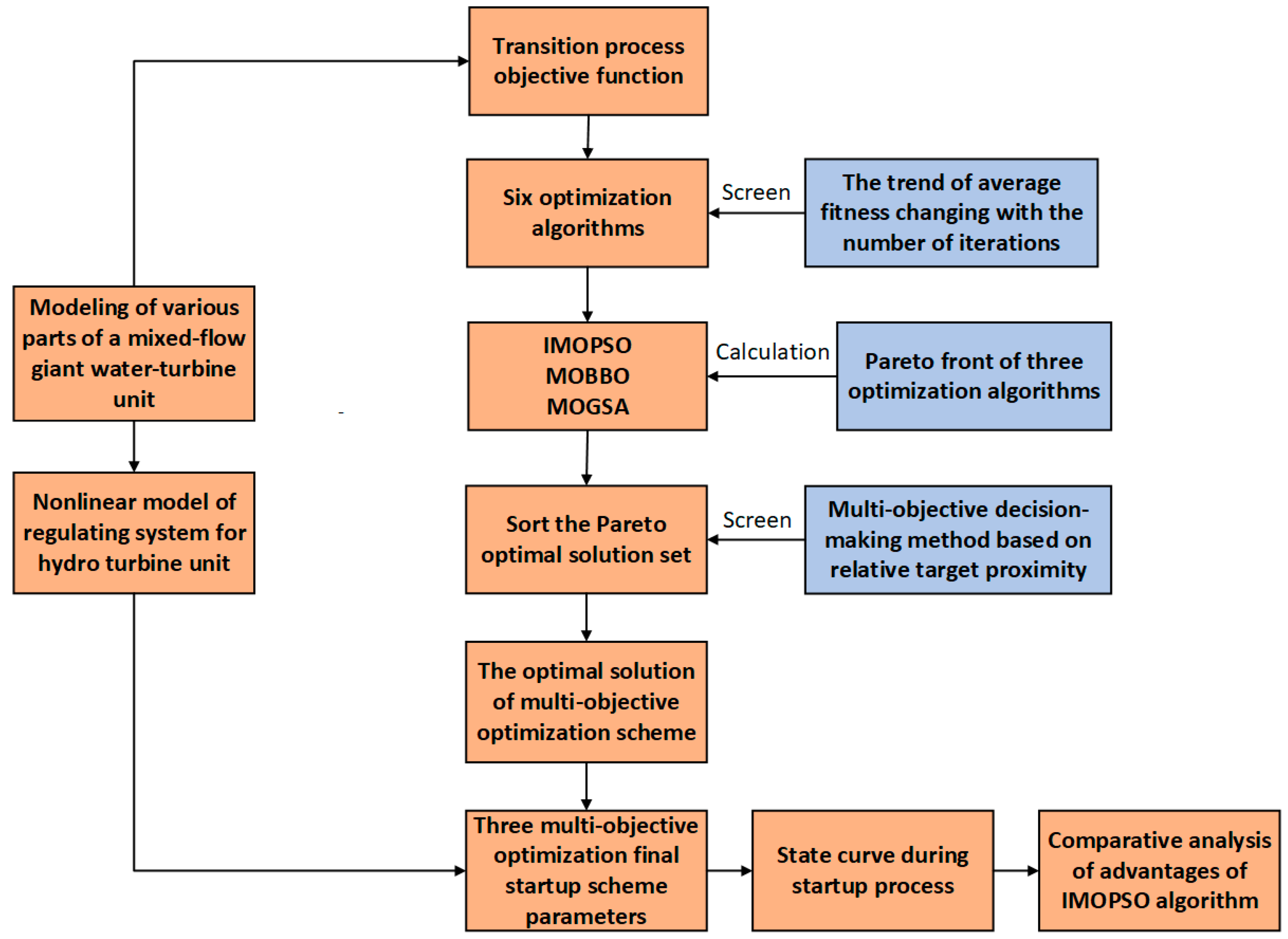
The structure of this article is as follows: the first part introduces the nonlinear modeling steps of giant hydropower units, including detailed descriptions and modeling methods of pressure diversion systems, PID and fractional-order PID controller models, actuators, turbine systems, and generator systems. The second part elaborates on the design and implementation of an improved multi-objective particle swarm optimization algorithm (IMOPSO), introducing the specific steps of the algorithm, neighborhood search strategy, and the improvement of solution diversity and global performance during the optimization process. The third part compares and analyzes various optimization algorithms, including MOPSO, MOSCA, MOBBO, MOGAS, and IMOPSO, and verifies the advantages and improvements of IMOPSO in optimizing the start-up process of hydropower units through experiments. The fourth part compares the simulation results with actual operating data, analyzes the performance of various optimization methods under different objective functions, and verifies the effectiveness of the improved multi-objective optimization method. The final section summarizes the main contributions and research findings of this article, and proposes possible directions for further research. The specific ideas and steps of the article are shown in Figure 1.

2. Hydropower-Unit Regulation System Model

This study establishes a nonlinear model of the regulation system for a large mixed–flow hydropower unit. The model primarily includes five modules: the water conveyance system, the micro-regulator, the actuator, the turbine, and the generator.

The composition of the model is illustrated in Figure 2.

2.1. Water Conveyance Pressure System

In practical engineering applications, the method of undetermined coefficients can be used to convert the characteristic line equations into a form of difference equations. Along the positive characteristic line of the water hammer, points A and P are considered, where the pressure wave propagation time from point A to point P is ∆t. Similarly, the pressure wave propagation time from point B to point P is also ∆t. This can be expressed as follows:

$$\{\begin{array}{l}(Q_P-Q_A)+{\displaystyle \frac{gF}{c}}(H_P-H_A)+{\displaystyle \frac{f\Delta t}{2DF}}{Q}_A\left|Q_A\right|=0\\ (Q_P-Q_B)-{\displaystyle \frac{gF}{c}}(H_P-H_A)+{\displaystyle \frac{f\Delta t}{2DF}}{Q}_B\left|Q_B\right|=0\end{array}$$

(1)

It can be simplified and expressed as follows:

$$\{\begin{array}{l}{C}^{+}:H_P=C_P-B{Q}_P\\ C^{-}:H_P=C_M-B{Q}_P\end{array}$$

(2)

In the equations, C_P = H_A + BQ_A - R|Q_A|Q_A, C_M = H_B + BQ_B − R|Q_B|Q_B.

In the equations, C⁺ and C⁻ represents the direction of the water hammer; H_i and Q_i represent the head and flow rate at the pipeline nodes, respectively; i denotes points A, B, and P; a is the wave speed; D is the diameter of the pipe; A is the cross-sectional area of the pipe; f is the friction coefficient; ∆x is the simulation step length; and g is the gravitational acceleration. Considering the actual length of the pipeline, it is divided into N segments in space, with each node represented by a sequence number and each segment having a length of ∆x. By substituting Equation (2) into the description of the divided pipeline and its boundaries, the iterative solution for the changes in head and flow rate throughout the entire pipeline can be obtained.

2.2. PID and Fractional-Order PID Controller Models

The block diagram of the fractional-order PID controller is shown in Figure 3, where λ and μ represent the orders of the integral and derivative, respectively. When λ = μ = 1, it becomes a conventional PID controller. In the simulation of the transition process in this study, the incremental PID control algorithm is used to discretize the PID controller for computer simulation [13]. When λ and μ are not equal to 1, the range of adjustment becomes broader due, to the change in the orders of the integral and derivative, allowing for more precise control over the system [14]. Equation (3) describes the system using the fractional-order PID controller:

$$u(t)=K_p\mathrm{e}(t)+K_i{\mathrm{D}}^{-\lambda }\mathrm{e}(t)+K_d{\mathrm{D}}^u\mathrm{e}(t)$$

(3)

2.3. Actuator

The actuator mainly consists of nonlinear components such as amplifying elements, the main control valve, and the main relay [15]. The transfer-function block diagram is shown in Figure 4, where T_y1 is the time constant of the main control valve, and T_y is the reaction time constant of the main relay.

2.4. Turbine System

The turbine is a complex nonlinear system. During the transition process, as the operating point of the turbine regulation system changes rapidly, the approximate values of the system transmission coefficients can cause significant cumulative errors when calculating the turbine torque and flow rate.

To overcome the above problem, the path integral process of the turbine torque and flow rate is improved, resulting in transient expressions for the turbine-torque and flow-rate dynamic equations.

Given the torque m_ta(x_a y_a h_a) at a known operating point a, the torque at any operating point d can be expressed as

$$m_{td}\left(x_d{y}_d{h}_d\right)=m_{ta}\left(x_a{y}_a{h}_a\right)+{\displaystyle \underset{x_a}{\overset{x_d}{\int }}{e}_{mx}dx}+{\displaystyle \underset{y_a}{\overset{y_d}{\int }}{e}_{my}dy}+{\displaystyle \underset{h_a}{\overset{h_d}{\int }}{e}_{mh}dh}$$

(4)

Similarly, given the flow rate q_ta(x_a y_a h_a) at a known operating point a, the flow rate at any operating point d can be expressed as

$$q_{td}\left(x_d{y}_d{h}_d\right)=q_{ta}\left(x_a{y}_a{h}_a\right)+{\displaystyle \underset{x_a}{\overset{x_d}{\int }}{e}_{qx}dx}+{\displaystyle \underset{y_a}{\overset{y_d}{\int }}{e}_{qy}dy}+{\displaystyle \underset{h_a}{\overset{h_d}{\int }}{e}_{qh}dh}$$

(5)

In summary, Equations (4) and (5) describe the transient characteristics of the turbine regulation system in terms of turbine torque and flow rate [16]. The transient expressions for torque and flow rate during the startup transition process of the turbine regulation system can be represented as

$$\{\begin{array}{l}{m}_t\left(x y h\right)=1.67yh-0.08x^2-0.3x+1.548(1-0.6x)y-0.279\\ q_t\left(x y h\right)=1.65y-0.5y^2-0.15x-(0.17+0.4y)T_w{q}^{\prime }-0.15\end{array}$$

(6)

where Q is the flow rate through the turbine; M is the torque generated by the turbine; and H is the working head of the turbine. Parameters m, q, h, x, and y represent the relative deviations of the parameters M, Q, H, N, Y, respectively.

2.5. Generator System

When the power plant operates in an isolated network, the generator and load can be represented using a first-order simplified model in the simulation calculations of the transient process of the hydropower generating unit, as shown in Equation (7):

$$T_a{\displaystyle \frac{dn}{dt}}+{\mathrm{e}}_n\left(n-n_r\right)=m_t-m_g$$

(7)

In the equation, T_a is the inertia time constant of the unit, n_r is the rated speed of the unit, n is the relative speed, e_n is the comprehensive self-regulation coefficient of the unit, mt is the main torque, and m_g is the resistance torque. In the modeling of this generator system, in order to simplify the operation and avoid the problem of the curse of dimensionality caused by high order, we only consider the first-order generator model. Regarding the impact of low-order models on the accuracy of the entire system, as the focus of this study is on the screening of multi-objective optimization algorithms themselves, the first-order generator model meets the requirements of this experiment.

The simulation model is shown in Figure 5.

3. Improved Multi-Objective Particle Swarm Optimization Algorithm

Particle Swarm Optimization (PSO) is an optimization algorithm based on swarm intelligence. Compared to traditional gradient-based optimization algorithms, PSO has a wide range of applicability, strong robustness, and extensibility, and offers fast search speeds [17]. Due to these performance advantages, many researchers have proposed the multi-objective particle swarm optimization (MOPSO) algorithm [18].

Compared to other multi-objective optimization algorithms, MOPSO is simpler in structure, easier to implement, and has faster convergence speeds. However, MOPSO, like other intelligent optimization algorithms, is prone to becoming trapped in local optima. To address this issue, this paper introduces an archive-based neighborhood search and proposes an improved multi-objective particle swarm optimization (IMOPSO) algorithm. The aim is to further enhance the convergence and distribution of the multi–objective particle swarm algorithm.

3.1. IMOPSO Algorithm Process

This paper introduces a neighborhood search strategy [19] into the standard multi–objective particle swarm optimization (MOPSO) algorithm. For each non–dominated solution in the external elite archive, a neighborhood search is conducted. The specific formula is as follows:

$$\{\begin{array}{l}{L}_1=L_0\left(B_u^d-B_l^d\right)\\ x_n^d=x_{rep}^d+L\left(rand-0.5\right)\end{array}$$

(8)

In the formulas, x^d_rep is the position of the individual in the external elite archive in the d-th dimension, x^d_n is the position of the individual generated by neighborhood search in the d-th dimension, and d = (d₁, d₂, …, d_r) is the set of r randomly selected dimensions from the external archive. The length of d will gradually decrease as the iterations progress. The specific formula for calculating r is as follows:

$$\{\begin{array}{l}r=D,n=0\\ r=D\ast e^{\delta \left({\displaystyle \frac{n}{n_{\max }}}\right)},0<n<0.8\ast n_{\max }\\ r=1,n>0.8\ast n_{\max }\end{array}$$

(9)

In the formulas, D is the dimensionality of the position vector of the individuals in the external elite archive, Max is the maximum number of iterations, and δ is the decay factor. [X] denotes the integer closest to X. The newly generated individuals from the neighborhood search strategy are combined with the original individuals in the external elite archive. All dominated individuals are deleted, and all non-dominated solutions are retained and stored in the elite archive.

The specific algorithm steps for the improved multi-objective particle swarm optimization (IMOPSO) proposed in this paper are as follows:

Step 1: Algorithm Initialization. Set the algorithm parameters, including population size N, elite archive size N_r, maximum number of iterations Max, inertia weight w, decay factor w_d, learning factors C₁ and C₂, and the number of grid divisions n_G. Determine the range for particle positions, randomly initialize the particle positions within this range, and initialize the particle velocities v to zero. Set the iteration counter t = 0.

Step 2: Evaluate the objective function values for each particle in the population using their position vectors x.

Step 3: Determine the dominance relationships among the particles in the population based on the Pareto dominance definition and select all non-dominated solutions to be stored in the elite archive.

Step 4: Perform adaptive grid division of the objective space in the elite archive and determine the grid positions of the particles, based on their objective function values.

Step 5: Initialize the personal best position P_best for each particle.

Step 6: Select the global best position G_best from the elite archive, based on the crowding distance in the objective space.

Step 7: Update the velocity and position of each particle using the following formulas:

$$\{\begin{array}{l}{v}_i^d(t+1)=w\ast v_i^d(t)+c_1\ast r_1(P_{ibest}^d(t)-x_i^d(t))+c_2\ast r_2(G_{best}(t)-x_i^d(t))\\ x_i^d(t+1)=x_i^d(t)+v_i^d(t)\end{array}$$

(10)

Step 8: Update the objective function values of the particles.

Step 9: Update the personal best positions P_best of the particles.

Step 10: Update the dominance relationships among the particles in the population and update the elite archive.

Step 11: Perform neighborhood search on all particles in the elite archive to generate new individuals and calculate their objective function values.

Step 12: Combine the newly generated individuals with the original individuals in the external elite archive, determine the dominance relationships among the individuals, and retain all non–dominated solutions in the elite archive.

Step 13: Re-perform adaptive grid division of the objective space in the elite archive and determine the grid positions of the particles.

Step 14: Check if the elite archive exceeds its maximum capacity. If it does, perform non-dominated solution pruning in the elite archive.

Step 15: Increment the iteration counter t = t + 1. If t $\le$ Max, go to Step 6. Otherwise, end the loop, and the elite archive will contain the Pareto optimal solutions.

3.2. Multi-Objective Decision-Making Method

The result of multi-objective optimization is a set of Pareto optimal solutions, where all particles in the Pareto optimal set are non-dominated with respect to each other. To facilitate decision-makers in selecting the optimal solution suitable for power plant operation from this set, this paper introduces the entropy weight method [20] to calculate the objective weights of each objective function. Additionally, subjective weights are assigned to each objective function, based on experience [21]. By combining the objective and subjective weights, the comprehensive weights are calculated. Finally, the concept of the ideal point is introduced. The method based on the relative closeness to the ideal solution [22] is used to calculate the distance between each particle in the Pareto optimal set and the ideal point. The particles in the Pareto optimal set are then ranked based on these distances, and the top-ranked particles are selected as the optimal solutions.

Assuming there are mmm particles in the Pareto optimal set and the probability of each particle appearing is Pi (i = 1, 2, …, m), the information entropy is defined as follows:

$$e=-\sum _{i=1}^m{p}_i\cdot \ln p_i$$

(11)

The entropy value reflects the degree of variation and the information content in the objective function. A lower entropy value signifies a higher degree of variation and information content, thereby increasing the objective weight. Conversely, the larger the entropy value, the smaller the objective weight.

The original data matrix formed by the Pareto optimal set is defined as follows:

$$R={\left(\begin{array}{cccc}{r}_{11}& r_{12}& \cdots & r_{1n}\\ r_{21}& r_{22}& \cdots & r_{2n}\\ ⋮& ⋮& \cdots & ⋮\\ r_{m1}& r_{m2}& \cdots & r_{mn}\end{array}\right)}_{m\times n}$$

(12)

In the matrix, R_ij represents the evaluation value of the i-th particle under the j-th objective function, m is the number of particles in the Pareto optimal set, and n is the number of objective functions.

The steps to calculate the objective weights and comprehensive weights of the objective functions are summarized as follows:

Step 1: Normalize the values of all particles in the Pareto optimal set:

$$\{\begin{array}{l}\overline{F}(X)=\left[{\displaystyle \frac{f_1(X)-d_{11}}{d_{12}-d_{11}}},{\displaystyle \frac{f_2(X)-d_{21}}{d_{22}-d_{21}}},\cdots ,{\displaystyle \frac{f_n(X)-d_{n1}}{d_{n2}-d_{n1}}}\right]\\ \overline{F}(X)=\left({\overline{f}}_1(X),{\overline{f}}_2(X),\cdots ,{\overline{f}}_n(X)\right)\end{array}$$

(13)

In the formula, R_j1 and R_j2 are the minimum and maximum values of the j-th objective function in the Pareto optimal set, respectively.

Step 2: Calculate the proportion P_ij of the objective function value of the i-th particle under the j-th objective function:

$$p_{ij}=r_{ij}/\sum _{i=1}^m{r}_{ij}$$

(14)

Step 3: Calculate the entropy ej of the j-th objective function:

$$e_j=-\left(\sum _{i=1}^m{p}_{ij}\cdot \ln p_{ij}\right)/\ln m$$

(15)

Step 4: Calculate the objective weight αj of the j-th objective function:

$${\alpha }_j=\left(1-e_j\right)/\sum _{j=1}^n\left(1-e_j\right)$$

(16)

Step 5: Combine the assigned subjective weight β_j with the objective weight α_j to calculate the comprehensive weight γ_j of the j-th objective function:

$${\gamma }_j={\beta }_j{\alpha }_j/\sum _{j=1}^n\beta {\alpha }_j$$

(17)

To further proceed, the concept of the ideal point is introduced. By combining the comprehensive weights of each objective function, the relative closeness method is used to calculate the distance between each particle in the Pareto optimal set and the ideal point. The specific steps are as follows:

Step 1: Normalize the values of each particle in the Pareto optimal set.

Step 2: Designate the optimal point as F_min = [d₁₁, d₂₁, …, d_n1] and the worst-case point as Fmax, denoted by F_max = [d₁₂, d₂₂, …, d_n2]. Proceed to normalize both the optimal and worst-case points.

Step 3: Combine the comprehensive weights γ_j to calculate the weighted distance g₁(X) from every particle in the Pareto optimal set to the ideal point, and also the weighted distance g₂(X) from each particle to the negative ideal point:

$$g_1(X)={\left\{\sum _{j=1}^n{\left[{\gamma }_j\left({\overline{f}}_j(X)-0\right)\right]}^2\right\}}^{{\displaystyle \frac{1}{2}}}$$

(18)

$$g_2(X)={\left\{\sum _{j=1}^n{\left[{\gamma }_j\left({\overline{f}}_j(X)-1\right)\right]}^2\right\}}^{{\displaystyle \frac{1}{2}}}$$

(19)

Step 4: Define the relative closeness l(X) of each particle to the ideal point, as follows:

$$l(X)={\displaystyle \frac{g_2(X)}{g_1(X)+g_2(X)}}$$

(20)

where l(X) indicates the relative closeness of the particle to the ideal point. A larger l(X) value indicates that the particle is closer to the ideal point, resulting in a higher ranking in the sorting order.

3.3. Objective Functions

To mitigate hydraulic fluctuations and mechanical vibrations during the startup process, this paper includes the water pressure fluctuations at the spiral case inlet and the axial water thrust in the objective functions. For overall stability during the startup process, speed and water pressure are normalized, and their deviations from the calibrated values are integrated over time to find the minimum integral value. Thus, the integral of the absolute value of the relative speed error (J₁), the integral of the absolute value of the relative water pressure error at the spiral case (J₂), and the maximum relative axial water thrust (J₃) are used as the objective functions for multi-objective optimization of the unit startup:

$$\{\begin{array}{l}{J}_1={\displaystyle \sum _{i=1}^k\frac{n\left(i\right)-n(\infty )}{n(\infty )}}\\ J_2={\displaystyle \sum _{i=1}^k\frac{H_{vol}\left(i\right)-H_{vol\_a}}{H_{vol\_a}}}\\ J_3=\max [{\displaystyle \frac{F_w(i)}{F_{wr}}}]\end{array}$$

(21)

In the formulas, k is the total number of samples, i is the sampling point, n(i) represents the sampled speed value, and n(∞) is the rated speed value, which generally corresponds to the steady-state speed value, H_vol(i) represents the sampled spiral-case water pressure value, and H_{vol_a} is the average spiral-case water pressure value; the calculation formulas are as follows:

$$H_{vol\_a}={\displaystyle \frac{{\displaystyle \sum _{i=1}^k{H}_{vol}\left(i\right)}}{k}}$$

(22)

The three objective functions—the relative speed error (J₁), the relative water pressure error at the spiral case (J₂), and the maximum relative axial water thrust (J₃)—reflect the speed increase, pressure fluctuations, and mechanical vibrations, respectively, during the actual startup process of the unit. The first objective function J₁ aims to minimize the integral of the absolute value of the relative speed error. The second objective function J₂ aims to minimize the integral of the absolute value of the relative water pressure error at the spiral case. The third objective function J₃ aims to minimize the maximum relative axial water thrust.

3.4. Selection of Decision Variables

Different startup patterns result in different hydraulic transition processes. For large mixed-flow turbine units, a two-stage startup pattern is generally adopted. As shown in Figure 6, the guide vanes are initially rapidly opened to Y₁ at a predetermined speed and held for a certain period before being closed at the fastest speed. When the unit speed reaches 90%, the governor enters idle operation, and PID control is activated. The guide-vane opening is then adjusted to point C.

The decision vector x = [K_p, K_i, K_d, Y₁, Y₂, t₁, t₂, t₃] is composed of the following optimization parameters: the proportional (K_p), integral (K_i), and derivative (K_d) parameters of the unit’s PID controller, the maximum no-load opening limit Y₁ and the corresponding guide-vane rise time t₁, the time t₂ when the guide vanes start closing, the opening Y₂ when the PID control is activated, and the corresponding time t₃. These parameters are selected as the decision variables for the optimization process.

3.5. Constraints

The constraint functions can be of several different types:

• Range restrictions on decision variables. This limits the setting range of the decision variables and can be represented as follows:

  $$x_i\in \left[X_{\min },X_{\max }\right]$$

  (23)

  where X_min and X_max represent the lower and upper bounds of the decision variables, respectively: X_min = [0, 0, 0, 0.15, 0.12, 5, 20, 20], X_max =[5, 1, 1, 0.3, 0.2, 20, 40, 50].
• Industry norms for parameter restrictions. By limiting the number of oscillations during the speed rise process, the vibrations at various parts of the unit during startup are kept within acceptable limits. T_u is the upper limit for regulation time. There are also restrictions on the setting of openings:

  $$\{\begin{array}{l}{t}_{a}z\le T_u\\ z\le 1\\ Y_1\ge Y_2\end{array}$$

  (24)

4. Engineering Case

Taking a large mixed-flow hydropower unit in Southwest China as an example, the improved multi-objective particle swarm optimization algorithm (IMOPSO) is used for multi-objective optimization of the startup pattern and PID control parameters under normal water head conditions. The results are compared with those obtained using multi-objective particle swarm optimization (MOPSO), variant multi-objective particle swarm optimization (VMOPSO), the multi-objective sine cosine algorithm (MOSCA), multi-objective biogeography-based optimization (MOBBO), the multi-objective gravitational search algorithm (MOGAS), and the improved multi-objective particle swarm optimization (IMOPSO). The average fitness-change curves of the six optimization algorithms are analyzed.

By selecting the algorithms with the fastest average fitness decline, further analysis and comparison are conducted on the control capabilities and dominant advantages of several non-dominated solutions in the Pareto front. This illustrates the flexibility and superiority of the improved multi-objective particle swarm optimization algorithm (IMOPSO) in practical applications. Some relevant data for the large hydropower unit are shown in

Table 2. Relevant parameters of the large hydropower unit.

Subsystems	Parameters
Governor	ep = 0.04; Ty = 0.459; Ty1 = 0.0408; Delay = 0.1 s; Dead Zone = 0.01 s
Turbine and Water Conveyance System	D = 6.223 m; Hr = 197 m; Hmax = 229.4 m; Hmin = 154.6 m; Qr = 432.7 m3/s; wr = 125 r/min; Tw = 0.873
Generator	Ta = 12.239; Dt = 1.5; w0 = 314; eg = 0.176

.

To avoid unnecessary computations, the optimization effectiveness of the IPSO algorithm is first tested and compared with particle swarm optimization (PSO), variant particle swarm optimization (VPSO), the sine cosine algorithm (SCA), biogeography-based optimization (BBO), and the gravitational search algorithm (GAS), using three objective functions. The three test functions are the integral of the absolute value of the relative speed error, the integral of the absolute value of the relative spiral-case water pressure error, and the maximum relative axial water thrust. The minimum value F_min of these objective functions is 0. The initial parameters of each algorithm are shown in

Table 3. Initialization parameters for optimization algorithms.

Optimization Algorithm	Population Size	Number of Iterations	Initial Parameter Settings
PSO	50	500	Initial Weights w0 = 0.8, Learning Rate c1 = c2 = 0.8
VPSO	50	500	Initial Weights w0 = 0.8, Learning Rate c1 = c2 = 0.8, Mutation Probability Pm = 0.01
SCA	50	500	Initial Amplitude r0 = 2
BBO	50	500	Mutation Probability Pm = 0.01, Retention Rate Rk = 0.2
GSA	50	500	Gravitational Constant G0 = 100, Decay Rate β0 = 20
IPSO	50	500	Initial Weights w0 = 0.8, Learning Rate c1 = c2 = 0.8, Neighborhood Search Step Size L0 = 0.1, Neighborhood Search Decay Coefficient δ = −2

, and the descriptions of the test functions are shown in

Table 4. Mathematical descriptions of the three test functions.

Test Functions	k	Domains
$J_1={\displaystyle \sum _{i=1}^k\frac{n\left(i\right)-n(\infty )}{n(\infty )}}$	50	[−100, 100] k
$J_2={\displaystyle \sum _{i=1}^k\frac{H_{vol}\left(i\right)-H_{vol\_a}}{H_{vol\_a}}}$	50	[−50, 50] k
$J_3=\max \left[{\displaystyle \frac{F_w\left(i\right)}{F_{wr}}}\right]$	50	[−100, 100] k

.

The average fitness-change curves for each algorithm, represented in logarithmic form, are shown in Figure 7. From the trend of the average fitness of each optimization algorithm as a function of the number of iterations in Figure 7, it can be seen that, compared to other algorithms, BBO, GSA, and IPSO show a sharp decline in average fitness and reach lower values, indicating higher accuracy. Therefore, to further compare the accuracy of the algorithms in multi-objective optimization problems, MOBBO, MOGSA, and IMOPSO are selected for comparative analysis.

MOBBO, MOGSA, and IMOPSO are selected for comparison to analyze the differences in the Pareto fronts among the three multi-objective optimization algorithms. To ensure the rationality of parameter settings, we referred to the settings and experimental methods of other related studies [23]. In this study, we conducted multiple independent experiments using similar methods to ensure the stability of the algorithm and the relative optimality of the parameters. Specifically, we systematically debugged and validated parameters such as population size, inertia weight, and acceleration coefficient, and ultimately obtained the optimal parameter combination for performance in the research environment. The parameter settings for the improved multi-objective particle swarm optimization algorithm (IMOPSO) are shown in

Table 5. IMOPSO algorithm parameter settings.

Parameters	Size	Meaning
M	20,000	Maximum Evaluations
N	50	Population Size
Nr	100	Elite Archive Size
nG	10	Grid Divisions
α	0.1	Grid Expansion Factor
β	2	Global Best-Selection Factor
γ	2	Elite Archive-Deletion Factor
w	0.5	Inertia Weight
wd	0.99	Inertia Weight-Decay Factor
C1	1	Learning Factor
C2	2	Learning Factor
L0	0.1	Archive Neighborhood Search Step Size
δ	−4.25	Archive Neighborhood Search Decay Factor

.

The Pareto fronts obtained by the MOBBO, MOGSA, and IMOPSO algorithms are shown in Figure 8 and Figure 9. These three multi-objective particle swarm optimization algorithms were used to optimize three key performance indicators of the hydropower unit. The performance of each algorithm during the optimization process, as well as their efficiency in maintaining the convergence, distribution, and coverage of the Pareto front, were compared.

The solution set of MOBBO exhibited certain limitations, primarily reflected in the concentrated distribution of solutions, with many tending to converge to local optimal regions. This indicates that the basic MOPSO algorithm is inefficient in exploring the global Pareto front and has limited ability to explore a broader solution space in multi-objective problems, making it prone to local optima.

MOGSA and IMOPSO, by introducing mutation mechanisms, adaptive grid partitioning, and elite archive strategies, significantly improved the diversity and global search capability of the solutions, effectively escaping local optima and discovering more potential non-dominated solutions. In optimizing the three key performance indicators—integral of the absolute value of the relative speed error, integral of the absolute value of the relative spiral-case water pressure error, and maximum relative axial water thrust—the two algorithms showed different strengths. The Pareto front generated by MOGSA was more extensive than that generated by IMOPSO, covering more extreme and edge values. The Pareto front generated by IMOPSO, however, was not only closer to the true Pareto front but also more compact and forward-looking in the multi-objective space, with higher convergence and superior Pareto-front quality.

The Pareto solution sets obtained by the three multi-objective particle swarm optimization algorithms combined the three objectives of the integral of the absolute value of the relative speed error, the integral of the absolute value of the relative spiral-case water pressure error, and the maximum relative axial water thrust. These solutions balanced the speed smoothness with the impact of water pressure fluctuations and axial water thrust on the unit, optimizing the speed rise process while suppressing hydro-mechanical vibrations, thereby providing effective decision support for the safe and stable operation of the power plant.

To further analyze and compare, a multi-objective decision-making method based on proximity to the ideal point is used to rank the Pareto optimal set. The top-ranked particles are selected as the optimal solutions for comparative analysis. First, the objective weights for each objective function are calculated using the entropy weight method. Then, subjective weights for each objective function are assigned based on the decision maker’s judgment. Finally, by normalizing each particle in the Pareto optimal set, the comprehensive weights for each objective function can be calculated [24]. The data and prototype of the modeling and simulation unit in this experiment are all from a giant mixed-flow water turbine unit in the southwest region. In the optimal decision, the subjective weights of each objective function are subjectively judged and given by the power station company based on local policies, field conditions, and historical data of the power station, to provide subjective weight values as a reference. The weights for each objective function in the three schemes are shown in

Table 6. The weight values of three schemes.

Weight	α	β	γ
MOBBO	[0.35, 0.55]	[0.72, 0.28]	[0.85, 0.15]
MOGSA	[0.45, 0.55]	[0.72, 0.28]	[0.85, 0.15]
IMOPSO	[0.45, 0.55]	[0.72, 0.28]	[0.75, 0.25]

.

Based on the comprehensive weights of each objective function provided in Table 6, the particles in the Pareto optimal set are ranked according to their relative closeness to the ideal point. The highest-ranked particle is selected as the optimal solution for the multi-objective optimization scheme. The optimal solutions for the two schemes are shown in

Table 7. Final parameters of multi–objective optimization startup scheme.

Parameters	MOBBO Scheme	MOGSA Scheme	IMOPSO Scheme
KP	4.13	3.566	3.764
KI	0.347	0.348	0.224
KD	0.670	0.213	0.181
Y1	0.31	0.30	0.29
Y2	0.22	0.21	0.21
T1	17.69	16.56	15.96
T2	31.86	32.99	33.76
T3	43.52	42.54	41.82
J1	581.97	568.20	576.51
J2	21.51	20.93	20.68
J3	1.233	1.128	1.119

.

The optimal solutions of three optimization algorithms were introduced into the nonlinear model of the fine control system of a giant water turbine unit, and the startup process state curves of the three optimization algorithms were obtained. Through simulation experiments, the advantages of their optimal solutions for the algorithm, compared to the other two algorithms, were explained with respect to multiple aspects, and the effectiveness of the improved multi-objective optimization method was verified.

By analyzing the data in Table 7 and the startup process-state curves in Figure 10, the following conclusions can be drawn:

• The multi-objective optimization strategy for startup patterns based on the MOGSA algorithm and the IMOPSO-based optimization strategy proposed in this paper both outperform the MOBBO optimization strategy. Both achieve good optimization results in terms of the integral of the absolute value of the relative speed error, the integral of the absolute value of the relative spiral-case water pressure error, and the maximum relative axial water thrust. These improvements enhance the control performance during the startup process. The speed in both algorithms schemes rises smoothly and reaches stability within 100 s, with no overshoot or significant oscillations.
• The three objective functions—integral of the absolute value of the relative speed error, integral of the absolute value of the relative spiral-case water pressure error, and maximum relative axial water thrust—are mutually conflicting, and cannot be optimized simultaneously. A multi-objective decision-making method based on relative closeness to the ideal point is used to rank the particles in the Pareto optimal set, selecting the top-ranked particle as the optimal solution for the multi-objective optimization scheme. The MOGSA algorithm’s optimal solution is superior in terms of the speed’s rapidity and stability (referring to the shortest time for the speed to reach and stay within a ±2% error range), taking 92.14 s. However, it performs relatively poorly in terms of pressure fluctuation severity and maximum axial water thrust optimization, with larger values for J₂ and J₃. The startup state curves for guide-vane opening and flow show more fluctuations compared to IMOPSO, failing to achieve the same smoothness. The IMOPSO algorithm’s optimal solution better suppresses internal water pressure fluctuations and the maximum axial water thrust in the unit and pipeline, although it slightly sacrifices speed rise rapidity, stabilizing at 96.4 s. Its J₁ value is slightly higher than the MOGSA algorithm’s optimal solution, but in terms of J₂ and J₃, the IMOPSO algorithm provides significantly better results. This conclusion is also verified by the startup-state curves, where the IMOPSO algorithm’s curves for guide-vane opening and flow are also smoother.
• All optimal solutions are obtained by calculating objective weights using the entropy weight method, then assigning subjective weights based on the decision maker’s judgment, and finally calculating comprehensive weights by normalizing each particle in the Pareto optimal set. If the power station has specific startup requirements, the operating personnel can reconfigure the subjective weights based on the actual situation to obtain new comprehensive weights and choose the appropriate startup scheme.

5. Discussion

Using the improved multi–objective particle swarm optimization algorithm (IMOPSO) for multi-objective optimization of startup rules and PID control parameters under normal water head conditions, a comparison is made with multi-objective particle swarm optimization (MOPSO), variant multi-objective particle swarm optimization (VMOPSO), the multi-objective sine cosine algorithm (MOSCA), multi-objective biogeography-based optimization (MOBBO), and the multi-objective gravitational search algorithm (MOGAS). The trend of average fitness change over iterations for each optimization algorithm shows that, compared to MOPSO, VMOPSO, and MOSCA, the average fitness of MOBBO, MOGSA, and IMOPSO drops sharply and reaches lower values, indicating higher accuracy. Using actual operational data from a large mixed-flow hydropower unit, the Pareto fronts for the optimization of MOBBO, MOGSA, and IMOPSO were analyzed. The startup scheme parameters were obtained using a multi-objective decision-making method, resulting in the state curves of the startup process. By analyzing the state curves of the startup process for the three optimization algorithms, the focus and advantages of MOBBO, MOGSA, and IMOPSO in multi-objective optimization were clarified.

The MOGSA algorithm is the best in terms of speed-increase speed and stability, achieving and maintaining stability within a ±2% error range in 92.14 s. However, its optimization effect on water pressure fluctuations and maximum axial water thrust is relatively poor; the IMOPSO algorithm performs well in suppressing water pressure fluctuations and maximum axial water thrust inside the unit and pipeline, but slightly sacrifices the speed of speed increase. At the same time, the optimal solution of the IMOPSO algorithm has significant improvements in the stability of PID control when the opening is connected and in the stability of flow fluctuations, compared to other algorithms. In summary, compared with the MOBBO and MOGSA algorithms, the multi-objective optimization solution of the IMOPSO algorithm better suppresses water pressure fluctuations and maximum axial water thrust inside the unit and pipeline, improves the speed of speed increase to a certain extent, and better suppresses the fluctuations of opening and flow. Compared with the optimal solution of other optimization algorithms, the IMPSO algorithm avoids local optimal solutions and improves optimization efficiency, showing significant advantages.

In this experiment, there are still some shortcomings. We only considered the advantages of various indicators of the IMOPSO optimization algorithm during the startup process, and did not consider and compare the complexity and time of the algorithm. In future research, we will further introduce complexity and computing power factors for analysis and comparison.

6. Conclusions

This study proposes a multi-objective optimization strategy for the startup of hydroelectric units based on nonlinear models, which significantly improves the dynamic response performance of the units. By optimizing the opening law of the guide vanes, the significant advantages of the IMOPSO algorithm in avoiding local optima and improving optimization efficiency have been verified. The results show that the IMOPSO algorithm can not only ensure a smooth and rapid increase in unit speed, but also effectively suppress pressure fluctuations and mechanical vibrations, thereby enhancing the reliability of the unit and extending its service life. This study provides important theoretical support and practical guidance for the optimization of the transition process of hydropower units, enabling power station operators to adjust strategies and choose the best startup plan, based on actual needs.