Power Supply Risk Identification Method of Active Distribution Network Based on Transfer Learning and CBAM-CNN

Abstract

With the development of the power system, power users begin to use their own power supply in order to improve the power economy, but this also leads to the occurrence of the risk of self-provided power supply. The actual distribution network has few samples of power supply risk and it is difficult to identify the power supply risk by using conventional deep learning methods. In order to achieve high accuracy of self-provided power supply risk identification with small samples, this paper proposes a combination of transfer learning, convolutional block attention module (CBAM), and convolutional neural network (CNN) to identify the risk of self-provided power supply in an active distribution network. Firstly, in order to be able to further identify whether or not a risk will be caused based on completing the identification of the faulty line, we propose that it is necessary to identify whether or not the captive power supply on the faulty line is in operation. Second, in order to achieve high-precision identification and high-efficiency feature extraction, we propose to embed the CBAM into a CNN to form a CBAM-CNN model, so as to achieve high-efficiency feature extraction and high-precision risk identification. Finally, the use of transfer learning is proposed to solve the problem of low risk identification accuracy due to the small number of actual fault samples. Simulation experiments show that compared with other methods, the proposed method has the highest recognition accuracy and the best effect, and the risk recognition accuracy of active distribution network backup power is high in the case of fewer samples.

1. Introduction

With the rapid development of China’s power industry, more and more power users have begun to use their own power sources, such as photovoltaic power generation systems, energy storage systems, self-supplied power plants, etc., in order to improve the reliability and economy of electricity. The distribution network is the main way to supply power to power users. Most of the medium- and low-voltage distribution systems in our country use the small current grounding system and, due to the distribution network electrical equipment, power supply lines are long and often fail and single-phase grounding faults account for 85% of the total number of faults. In addition, because China, along with the user side of a large number of self-provided power supplies, continues to access the distribution network, the analysis of the operation status of the distribution network is more and more complex, and the evolution principle of the distribution network fault risk is more and more complex, which leads to the fault line being difficult to find. At the same time, there are still some areas using manual line selection methods to locate the line where single-phase grounding faults occur, and there are also grid maintenance personnel involved in the removal of faulty lines for maintenance of electrocution casualties [1]. Due to the maintenance, the fault line and the grid connection are cut off, but there may still be self-powered users on the line unaware of the electric power supply to the line, which ultimately leads to electric shock and casualties of maintenance personnel. This creates a risk when supplying self-power in an active distribution network. Therefore, it is necessary to study a more accurate method of identifying the risk of self-supplied power in active distribution networks, which is divided into two parts, one is to identify the faulty lines in the distribution network, and the other is to judge whether there is a self-supplied power supply on the faulty line to supply electricity. If both of them are satisfied, it means that there is a risk of supplying electricity.

Since transient features contain rich fault information, most scholars use transient features for research by combining the discrete Fourier transform [2], wavelet analysis [3,4], S-transform [5], and other methods [6,7] to process the transient signal and obtain the fault feature quantity to be used as the basis of fault line identification. However, the methods mentioned above are mainly used to extract features manually, and the selection of feature parameters will directly affect the identification of fault lines in the entire distribution network, and the extraction process will be relatively complex and time-consuming, which will affect its accuracy [8]. In addition, the literature [9,10,11] proposes grid fault identification and diagnosis through multi-agent systems (MASs), but this method has high requirements on the transmission delay of the communication, and the system structure is complex and costly to implement.

With the development of artificial intelligence, many scholars at home and abroad began to apply machine learning and deep learning to electrical engineering and other fields [12,13,14,15,16,17], which can solve the problems of low accuracy and weak robustness of traditional methods [18]. The literature [19] provides a study of single-phase ground fault routing for distributed networks based on the k-nearest neighbor classification (KNN) algorithm and, through the fault data processing to select the fault feature quantity, combined with the KNN algorithm for fault line routing, the KNN model is often used to deal with the nonlinear classification problem. The selection of the K value will have a huge impact on the classification results. When the collected samples are disturbed, the classification results are affected by outliers due to insufficient feature mining, and the accuracy of the results is low. A study [20] built a deep neural network (DNN) based on the Keras framework, which is a simple modeling method, but due to its simple network structure, it cannot extract fault features in a more comprehensive way, and thus its accuracy rate is low. A study [21] shows that China’s ultra-high-voltage AC and DC transmission system structure and fault characteristics are becoming more and more complex and, in order to achieve a complex grid and large data volume to accurately extract the fault characteristics, put forward a CNN based on the grid fault diagnosis method. However, the model’s ability to resist interference is not strong, and the method requires a large number of fault samples. In the actual environment of the interference signal and when the number of fault samples is small, it is difficult to achieve the model operation requirements. A study [22] combines the S-transform with the CNN to propose a new fault routing method for the CNN with strong anti-noise ability and high generalization level. However, the training of the deep learning model needs to rely on a large amount of data, but in the actual situation, the distribution network faults comprise only a small sample, and it is difficult to obtain a large number of historical data under the fault condition as the training sample to train the model, Therefore transfer learning is required. Most of the above methods for active distribution networks only consider accurate and fast fault finding of faulty lines without further consideration of identifying the presence or absence of captive power supply on the faulty line, although the risk of captive power supply may arise due to the fact that the captive power supply is still supplying power when the maintenance personnel carry out the maintenance, resulting in accidental electrocution of the maintenance personnel.

In order to be able to further determine whether there is a risk of self-powered supply based on the identification of the faulty line, we therefore need to identify whether the self-powered supply on the faulty line is in operation. In order to achieve high-accuracy recognition and feature extraction efficiency, we propose a combination of CBAM and CNN, which achieves automatic extraction of fault risk features by the CNN and enhances local feature extraction using the CBAM, thus achieving high-efficiency feature extraction as well as high-accuracy risk recognition. Due to the small number of actual fault samples, in order to solve the problem of low accuracy of risk identification in the case of small samples, this paper finally proposes the power supply risk identification method of an active distribution network based on transfer learning and CBAM-CNN.

Firstly, a convolutional neural network with embedded attention mechanism is constructed to extract the fault risk features in the transient zero-sequence current, and secondly, the transfer learning method is used to effectively solve the problem of low accuracy of risk identification of self-provided power supply with few samples. Finally, the active distribution network with self-contained power supply is constructed in Matlab/Simulink and compared with other methods to prove the effectiveness of the proposed method. The contribution of this work is summarized as follows:

• In order to be able to complete the identification of the faulty line and further identify whether it poses risks such as electrocution of maintenance personnel, we completed the identification of the self-supplied power supply on the faulty line. Compared with the selection of faulty lines only, this method is more comprehensive and helps to reduce the risk of supplying power from the self-provided power supply.
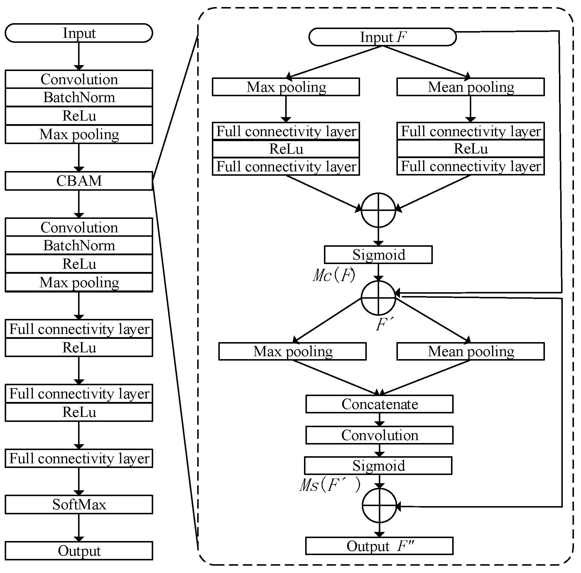
• We propose a combination of CBAM and CNN to achieve active extraction of fault risk features through the CNN and to enhance local feature extraction using the CBAM, so as to achieve high-efficiency feature extraction as well as high-accuracy risk identification.
• We propose a method combining transfer learning and CBAM-CNN, which can maintain a high recognition accuracy despite small samples and solve the problem of low risk recognition accuracy caused by few fault samples in real situations.

2. Transfer Learning

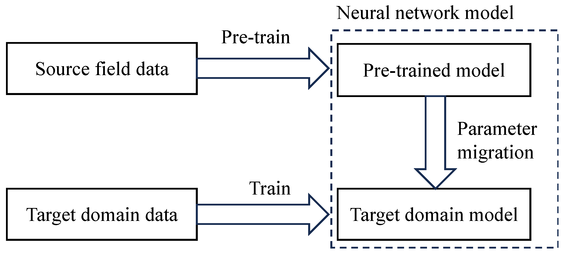
2.1. Principles of Transfer Learning

The essence of transfer learning is a learning process that takes advantage of similarities in models, data, or tasks to apply models learned and completed in an old domain to a new domain [23]. There are two important concepts [24]: domain and task. Domain: the sample dataset on the domain contains input x and output y, whose distribution can be written as P(x,y). The available formula is D = {X, Y, P(x,y)}, where X, Y denote the feature and labeling space in which the data samples are located, respectively. Task: for a given domain, the task T consists of two parts: the label space Y and the prediction function f(*) obtained through training, which can be expressed by the formula T = {Y, f(*)}. For transfer learning, both the domain and the task contain two parts: the source domain (Ds) and the source task (Ts), relative to the task trained in the old domain; and the target domain (Dt) and the target task (Tt), relative to the untrained task in the new domain. The transfer learning structure is illustrated in Figure 1.

2.2. Convolutional Neural Network Pre-Training Process

The flow chart of the pre-training of the convolutional neural network is shown in Figure 2.

In the downsampling layer, the features are extracted twice by sampling kernel b using the mean sampling method as shown in Equation (1).

$$y_i^L=x^{L-1}\otimes {\displaystyle \frac{1}{b}}$$

(1)

where L is the number of network layers, $y_i^L$ is the output feature surface of the convolutional layer, $x^{L-1}$ is the feature surface of the L-1 layer, and $\otimes$ is the sliding convolutional process.

Feedforward propagation is the prediction classification through the network. The process can then be seen as a feedforward operation.

$$w^n=f_{\mathrm{s}2}\left(f_{\mathrm{c}2}\left\{f_{\mathrm{s}1}\left[f_{\mathrm{c}1}\left(w^1\right)\right]\right\}\right)$$

(2)

where $w^1$, $w^n$ are the inputs and outputs, respectively, $f_{\mathrm{c}}$ is the convolutional operation, and $f_{\mathrm{s}}$ is the downsampling layer.

Error backpropagation compares the results with the labels, calculates the error between, and backpropagates it to the layers to update the weight parameters.

$$E^{\prime }=E+f_{\mathrm{BP}}(\alpha e^n)$$

(3)

where $E$ and $E^{\prime }$ are the parameters before and after the update, respectively, $f_{\mathrm{BP}}$ is the feedback calculation process, $\alpha$ is the learning rate, and $e^n$ is the error.

2.3. CNN Pre-Trained Based on Transfer Learning

For new tasks with insufficient training samples, transfer learning can put the trained source domain model into the new task to identify risks. The steps are to save the trained network weight parameters, migrate the parameters to the target domain, and train the target domain on the new classification task. It solves the problem of insufficient samples in the target domain and the cost of obtaining training samples.

Supervised training of the CNN is to use the processed source domain data and continuously update the weights through feedback operations to obtain a pre-trained model suitable for the source domain data. Due to the difference between the source domain data and the target domain data, the pre-training cannot be directly applied to the target domain, so it is necessary to migrate the pre-trained model to the target domain, as shown in Figure 3.

3. Risk Identification Model for Self-Provided Power Supply Integrated with Attention Mechanism

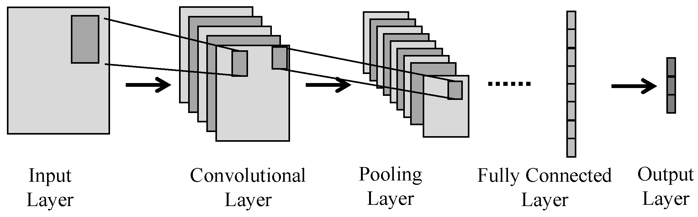
3.1. Convolutional Neural Network

In order to better mine the fault risk features, a CNN is used for feature extraction. A CNN is generally composed of convolutional layer, pooling layer, and fully connected layer [25]. The structure of the CNN is shown in Figure 4, where the input sample data are a one-dimensional waveform signal, and the network learns layer by layer to extract the features embedded in the data and finally outputs the probability of the sample belonging to the category through the fully connected layer and output layer.

3.1.1. Convolutional Layer

The purpose of the convolutional layer is to learn the feature representation of the input data and to generate the feature map by locally extracting the input features through convolutional computation using a convolutional kernel. The formula for convolution operation is given in Equation (4).

$$Y_{ij}=f({\displaystyle \sum _{i=1}^k{\displaystyle \sum _{j=1}^k(X_{ij}K)}}+b)$$

(4)

where Y_ij and X_ij are the elements involved in the computation in the input feature map and output feature map, respectively, b is the bias, K is the convolutional kernel, and f is the activation function.

3.1.2. Pooling Layer

The pooling layer, also known as the downsampling layer, has the role of secondary extraction of features, which can effectively reduce the size of the parameter matrix, improve the computational speed, and prevent the input of high-dimensional data to the next layer caused by the overfitting phenomenon. The two commonly used pooling operations are mean pool and max pool. Average pooling will be the average of a region instead of the region, the maximum pooling is to use the maximum value instead. Their operational formulas are shown in Equations (5) and (6).

$$p_A={\displaystyle \frac{1}{W}}{\displaystyle \sum _{t=(j-1)W+1}^{jW}{a}^{r(i,t)}}$$

(5)

$$P_M={\max }_{(j-1)W+1\le t\le jW}\left\{a^{r(i,t)}\right\}$$

(6)

where W is the width of the pooled layer region and $a^{l(i,t)}$ is the activation value of the t-th neuron in the i-th frame of the r-th layer.

3.1.3. Fully Connected Layer

The purpose is to classify the features extracted by the previous network. Generally there will be one or more fully connected layers behind the network, which are used to connect all the neurons of the previous layer to the neurons of the current layer, and finally its output is propagated to the output layer, and the classification result is expressed as a probability value between 0 and 1 through the Softmax function [26], to achieve the classification and recognition. The mathematical expression of the fully connected layer is shown in Equation (7):

$$z_k^{r+1}={\displaystyle \sum _{i=1}^n{w}_{ik}^r}{a}^{r(i)}+b_k^r$$

(7)

where $z_k^{r+1}$ is the logits value of the k-th output neuron in the r + 1 layer, $w_{ik}^r$ and $b_k^r$ are the weight and bias between the i-th neuron in the r-th layer and the k-th neuron in the next layer, respectively.

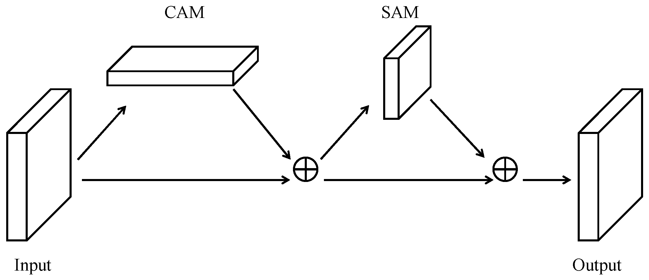
3.2. Convolutional Neural Networks That Fuse Attention Mechanisms

Since the pooling operation loses the location information of the feature, this will have an impact on the time series that is sensitive to the data series. To this end, the CBAM is used to extract and reduce the dimensionality of key features and data dimensions, as shown in Figure 5 [27].

The feature map of the CNN contains a wealth of attention information not only in the channel but also in the feature map inside the channel. Compared with other attention mechanisms, the CBAM constructs two sub-modules: spatial attention module (SAM) and channel attention module (CAM), to summarize and fuse attention information from spatial and channel aspects, respectively, so as to obtain more comprehensive attention information. The main implementation steps are as follows:

(1) The input original feature map is recorded as $F\in R^{C\times H\times W}$, where H and W represent the height and width of the input feature map, respectively, and C is the number of channels. The global spatial information of feature map F is compressed by adaptive average pooling and adaptive maximum pooling, and two feature maps S1, S2 with size C × 1 × 1 are generated.

(2) Channel attention mechanism. In order to aggregate the overall information of the feature maps in the convolutional neural network, the channel attention mechanism is used. It can make full use of the feature information extracted by the compression operation and obtain the correlation between channels. S1, S2 obtained two one-dimensional feature maps by sharing a multi-layer perception (MLP) composed of two fully connected layers and a ReLU nonlinear activation function. After summing the two graphs by channel, the sigmoid function is used to normalize the output value $M_c\left(F\right)$ of each channel of size C × 1 × 1. The mathematical expression for the above process is as follows in Equation (8):

$$M_{\mathrm{C}}\left(F\right)=\sigma \left\{g\left[P_{\mathrm{A}}(F)\right]+g\left[P_{\mathrm{M}}(F)\right]\right\}$$

(8)

where $\sigma$ is the sigmoid function, P_A is the average pooling operation, and P_M is the maximum pooling operation. g is the multi-layer perceptron.

a. The process of average pooling of the feature map F is shown in Equation (9).

$$P_{\mathrm{A}}(F)={\displaystyle \frac{1}{H\times W}}\sum _{i=1}^H\sum _{j=1}^W{f}_x(i,j)$$

(9)

where H, W represent the height and width of the CBAM input feature map, respectively, and $f_x\left(i,j\right)$ is the value of the pixel at point $\left(i,j\right)$ in the input feature map F channel x with coordinates.

b. The process of maximum pooling of the feature map F is shown in Equation (10):

$$P_M(F)=\underset{i\in H,j\in W}{\max }{f}_x(i,j)]$$

(10)

where H, W represent the height and width of the CBAM input feature map, respectively, and $f_x\left(i,j\right)$ is the value of the pixel at point $\left(i,j\right)$ in the input feature map F channel x with coordinates.

c. In the MLP, each neuron receives the output of the previous layer and performs weighted sum and activation function operations to obtain the output of the current layer. Commonly used activation functions are the sigmoid function, ReLU function, and so on. The role of the activation function is to introduce nonlinear factors in the output of the neuron so that the multilayer perceptual machine can learn more complex patterns. The sigmoid function is shown in Equation (11).

$$Sigmoid\left(x\right)={\displaystyle \frac{1}{1+e^{-x}}}$$

(11)

Finally, the feature maps after maximum pooling and average pooling are nonlinearly normalized by a sigmoid function to obtain the channel weight values $M_{\mathrm{c}}\left(F\right)$, which are inputted into the SAM.

(3) Spatial attention mechanism. Multiply the input feature map F by the weight value Mc(F) of each channel to obtain the feature map F′, which can effectively reflect the key channel information. Taking the feature map F′ obtained after channel feature recalibration as input, the average pooling and maximum pooling operations were performed in the channel dimension, and the feature maps $P_1\in R^{\mathrm{l}\times H\times W}$ and $P_2\in R^{\mathrm{l}\times H\times W}$ were obtained and then stitched together. The convolutional layer is used to encode and fuse the information of different positions in P₃ to obtain the spatially weighted information Ms(F′), which is used to distinguish the importance of different spatial positions of the image. The mathematical expression for the above process is as follows in Equation (12).

$$M_{\mathrm{S}}\left(F^{\prime }\right)=\sigma \left\{h\left[P_{\mathrm{A}}\left(F^{\prime }\right);P_{\mathrm{M}}\left(F^{\prime }\right)\right]\right\}$$

(12)

where h denotes the convolutional layer, $\sigma$ is the sigmoid function, F′ is the feature map. h denotes the convolutional layer, P_A is the average pooling operation, and P_M is the maximum pooling operation. “;” is the operation of splicing two feature maps.

The input feature map F′ was multiplied by the weight value Ms(F) of each channel to obtain the salient feature map output F″, which could contain channel position information and spatial position information, so as to improve the feature learning and expression ability of the model. Figure 6 shows the fault line selection model of CBAM-CNN with the fusion attention mechanism constructed in this paper.

4. Risk Identification of Self-Provided Power Supply in Distribution Network Based on Transfer Learning

In order to realize the identification of power supply risks in active distribution networks under small sample conditions, the method of transfer learning and a convolutional neural network is used to accurately identify them.

The CBAM-CNN model based on the transfer learning method is used to identify the risk of self-provisioned power in the active distribution network, which firstly needs to identify the faulted lines of the active distribution network. Secondly, in order to prevent the risk of electrocution casualties caused by the self-provisioned power supply on the lines still running into the distribution network during maintenance, it is necessary to identify whether there is any self-provisioned power supply sent out from the faulted line, and finally the self-provisioned power supply risk is identified. Figure 7 shows the risk identification process of self-provided power supply in the distribution network based on transfer learning.

5. Simulation Analysis

5.1. Case Design

The distribution network model is constructed in the preparation stage, and a large number of CNN-oriented distribution network fault data samples are generated by means of automated simulation.

Due to the fact that the amplitude of the transient zero-sequence current is larger and shorter in duration than the steady state value, and that the amplitude of the transient zero-sequence current is the largest in the grounding line, and its phase is still exactly opposite to the other lines, the zero-sequence current is chosen as the characteristic quantity for sampling [28].

Since the most widely used self-supplied power source in China is the photovoltaic (PV) system, and a single category of power source can simplify the distribution network model, the PV system is chosen for the self-supplied power source in the distribution network model. A complete self-supplied power module includes a self-supplied power supply and an energy storage battery. The self-supplied power supply stores some of the electrical energy in the low valley of electricity consumption, and when the self-supplied power supply suddenly does not work, it can supply power to the user through the battery to prevent the damage caused by the sudden change in voltage to the user’s electrical equipment, so the PV power generation system mainly includes the PV power generation module and the energy storage battery module.

Since our study area is northeast China, the widely used 66 kV/10 kV is selected as the distribution grid level. A model of a four-outlet (L = 4) 10 kV distribution network containing four captive power sources was constructed to simulate the risk of captive power supply as shown in Figure 8, where Q_L and C_L are the lengths of the overhead line and cable line, respectively, and the main feeder parameters in the network are shown in

Table 1. Feeder parameters.

Feeder Types	Phase Sequence	L (mH/km)	r ($\mathbf{\Omega }$/km)	C (μF/km)
Cable feeder	Positive sequence	4.6	0.135	0.0056
	Zero sequence	1.3	0.275	0.0095
Overhead feeder	Positive sequence	0.28	0.25	0.338
	Zero sequence	1.018	2.7	0.28

. Since the arcing coil is operated with over-compensation in most cases, here the compensation degree is taken as =10%, and the value of the arcing coil can be obtained as 15.8H from Equation (13) [29].

$$L={\displaystyle \frac{1}{(1+\rho )\cdot 3{\omega }^2{C}_{\mathsf{\Sigma }}}}=15.8\mathrm{H}$$

(13)

where $\rho$ is the overcompensation factor, $C_{\mathsf{\Sigma }}$ is the sum of distributed capacitances [29].

In order to generate massive fault samples to support the training process of the neural network, the Matlab batch automated simulation method is used to perform batch automated simulation by randomly changing the parameters of the distributed network. The detailed automation algorithm flow is shown in

Table 2. Automated simulation process.

Steps	Fault Automation Simulation Based on Matlab
1	Modeling of 10 kV distribution network with captive power supply through Matlab/Simulink tool
2	Parameter setting: divided into two categories with or without self-supplied power, each category has a randomly set fault location, fault phase angle, grounding resistance value
3	Start the simulation
4	Stop the simulation after 0.2 s of running
5	Automatically saves the zero-sequence current simulation data of L lines as a CSV file
6	Repeat steps 2–5 to generate the required number of samples for each type of fault
7	Repeat step 6 to obtain N class samples

.

According to the above simulation parameters, the single simulation time is 0.2 s and the sampling frequency is 1000 Hz, so 200 data points can be collected in one simulation, and 1080 fault scenarios were set up to generate source domain data, including different fault lines, fault locations, fault ground resistance, fault initial phase angle, and whether there is a self-provided power supply. The sample parameters are shown in the following

Table 3. Sample parameter.

Type	Faulty Lines	The Location of the Fault (%)	Faulty Ground Resistance (Ω)	Fault Initial Phase Angle (°)	Self-Provided Power
Parameter	L1 L2 L3 L4	10 20 30 40 50 60 70 80 90	0.01 10 100 500 1000	0 30 60 90	Yes
					No

.

In this paper, the collected three-phase currents are processed as zero-sequence currents in the form of one-dimensional vectors, which are input into the model as dataset samples.

At time t, the zero-sequence current can be obtained as:

$$I_l^0(k)={\displaystyle \frac{1}{3}}(I_l^A(t)+I_l^B(t)+I_l^C(t))$$

(14)

where $I_l^A(t),I_l^B(t),I_l^C(t)$ are the phase currents of A, B, and C.

Arrange the sampling points in combinations:

$$I_l^0=[I_l^0(1),I_l^0(2),\dots ,I_l^0(T)]$$

(15)

where T is the maximum time sampling point.

The fault characteristics of L outgoing lines are extended to form a one-dimensional vector form:

$$g=[I_1^0,I_2^0,\dots I_L^0]$$

(16)

where $g$ is the fault sample representing the zero-sequence current data of the i-th ($i=1,2,\dots ,L$) zero-sequence current data of the feeder.

Eventually, the size of each sample is M = 1 × 200 × L), and the size of the dataset is N = 1080 × M. In this study, the distribution network outgoing line L is 4, so M = 1 × 800 and N = 1080 × 800.

In order to eliminate the problem of data being flooded during training due to dimensional and order of magnitude differences between data, the original data need to be normalized, and the values of each processed data point are within 0–1. In this data pre-processing, the mean normalization method is used, and its main calculation method is as shown in Equation (17).

$$x={\displaystyle \frac{x-x_{\mathrm{m}ean}}{x_{\max }-x_{\min }}}$$

(17)

where $x$ is the dataset, $x_{\mathrm{mean}}$ is the sample mean, $x_{\max }$ and $x_{\min }$ are the maximum and minimum values, respectively.

5.2. Comparative Analysis of Test Results in the Source Domain

In this paper, the accuracy (A) is used as the model evaluation index to evaluate the recognition accuracy of the model, and the calculation formula is as follows:

$$A={\displaystyle \frac{T_{\mathrm{P}}+T_{\mathrm{N}}}{T_{\mathrm{P}}+T_{\mathrm{N}}+F_{\mathrm{P}}+F_{\mathrm{N}}}}$$

(18)

where a true positive $T_P$ represents the number of samples that are actually positive and the prediction is also positive; true negative $T_N$ indicates the number of samples that are actually negative and predicted to be negative; false positive $F_P$ indicates the number of samples that are actually negative and predicted to be positive; false negative $F_N$ indicates the number of samples that are actually positive and predicted to be negative.

5.2.1. Accuracy of Risk Identification of Self-Provided Power Supply

The CBAM-CNN proposed in this paper is used to identify the risk of self-provided power supply in the distribution network shown in Figure 8, which is divided into two parts: identifying fault lines and identifying whether fault lines have self-provided power supply. The effects of different transition resistances, different fault initial phase angles, and different fault distances on the performance of the source domain pre-trained model are verified.

When the fault occurs at 50% of the line and the initial phase angle of the fault is 0°, the fault resistance is set to 1 Ω, 50 Ω, and 300 Ω, respectively; when the fault ground resistance is 10 Ω and the fault occurs at 50% of the line, the fault initial phase angle is set to 20°, 45°, and 180°, respectively; when the fault ground resistance is 10 Ω and the fault initial phase angle is 0°, the fault distance is set at 25%, 45%, and 85% of the fault branch.

Table 4. Evaluation of the effectiveness of the model.

Fault Parameters	Value	Fault Line Accuracy	Power Supply Identification Accuracy
Fault resistance (Ω)	1	100	100
	50	100	100
	300	100	100
Fault initial phase angle (°)	20	100	100
	45	100	100
	180	100	100
Location of the fault (%)	25	100	100
	45	100	100
	85	100	100

shows the accuracy of fault line selection obtained by the method proposed in this paper in the above three cases.

5.2.2. Effectiveness of Noise Immunity

In order to verify the adaptability of the self-provided power supply risk identification method to the noise, in this paper, Gaussian noise with different signal-to-noise ratios (SNRs) is added to test and verify the proposed method under each fault scenario set in

Table 5. Recognition accuracy at low noise levels.

Noise Level/dB	Fault Line Accuracy	Power Supply Identification Accuracy	Noise Level/dB	Fault Line Accuracy	Power Supply Identification Accuracy
20	98.81%	99.73%	40	98.32%	99.51%
30	99.1%	99.16%	50	99.71%	99.65%

and

Table 6. Recognition accuracy at high noise levels.

Noise Level/dB	Fault Line Accuracy	Power Supply Identification Accuracy	Noise Level/dB	Fault Line Accuracy	Power Supply Identification Accuracy
60	96.51%	96.24%	100	94.02%	93.51%
80	94.71%	95.32%	120	91.21%	91.08%

.

The above results show that the performance of the model is basically not affected by the fault resistance, fault initial phase angle, and fault location and it has good adaptability to the low noise of the measurement data.

As can be seen from Table 6, the performance of the model decreases significantly when the measured data are subjected to higher noise, and the recognition accuracy is not too high. It is surmised that when faced with large disturbances such as high wind and rain or thunderstorms, the performance of the present model may be affected.

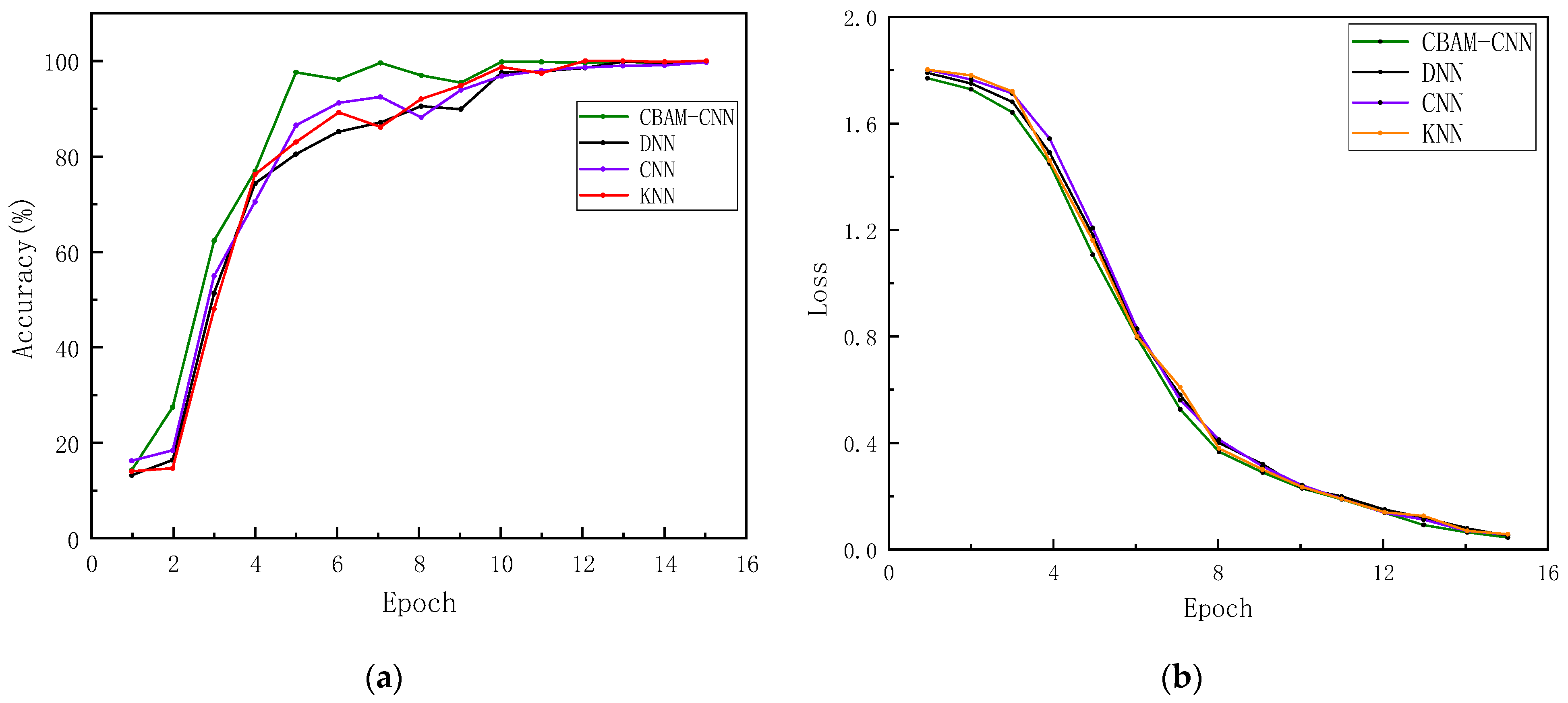
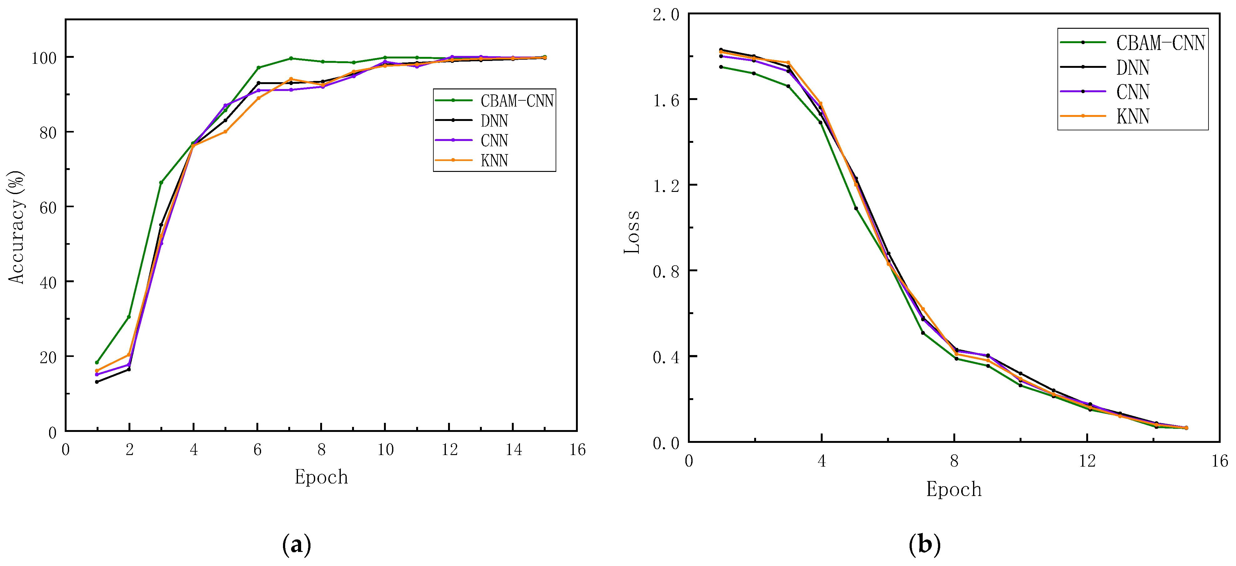
5.2.3. Analysis of the Effectiveness of the Risk Identification Network Model

In order to validate the effectiveness of the CBAM-CNN fault selection model as well as the power identification model proposed in this paper on the source domain dataset, comparative simulations of fault routing and power identification between the CNN, DNN, and KNN models and the scheme proposed in this paper are set up as shown in Figure 9 and Figure 10.

From Figure 9, it can be seen that the fault line selection model based on the CNN, KNN, and DNN needs about 10 epochs to converge, while the CBAM-CNN fault line selection model with the addition of the attention mechanism needs only 5 epochs to converge, and from Figure 10, it can be seen that the CBAM-CNN self-supply power supply identification model still converges faster than with the use of CNN, DNN, and KNN models, and the accuracy is slightly improved. It can be seen that the introduction of the attention mechanism in the CNN model can accelerate the convergence speed of the model, and the accuracy is also improved.

5.3. Comparative Analysis of Test Results in the Target Domain

Currently, most models mainly rely on a large amount of simulation data for training, and the problem of small sample size must be faced from the simulation platform to the actual application process. Therefore, transfer learning is needed. In this subsection, neutral ungrounded and small resistance grounding systems are set to generate target domain data, and their sample parameters are set the same as in Table 3, and each grounding method contains 1080 fault scenarios. The main process is as follows:

(1) Data pre-processing is carried out on the measurement data of the target power supply risk scenario and the target domain dataset is generated;

(2) Transfer the CBAM-CNN model weight parameters of the extracted features from the source model to preliminarily construct the target domain model;

(3) The target domain model is trained and tested by using the domain data to complete the target domain model construction.

Through the above process, this subsection first analyzes the sensitivity of the proposed scheme to the data volume of the unlabeled target domain, then analyzes the impact of different risk identification schemes on the model effect, and finally tests the effectiveness of the model in different distribution network operation scenarios.

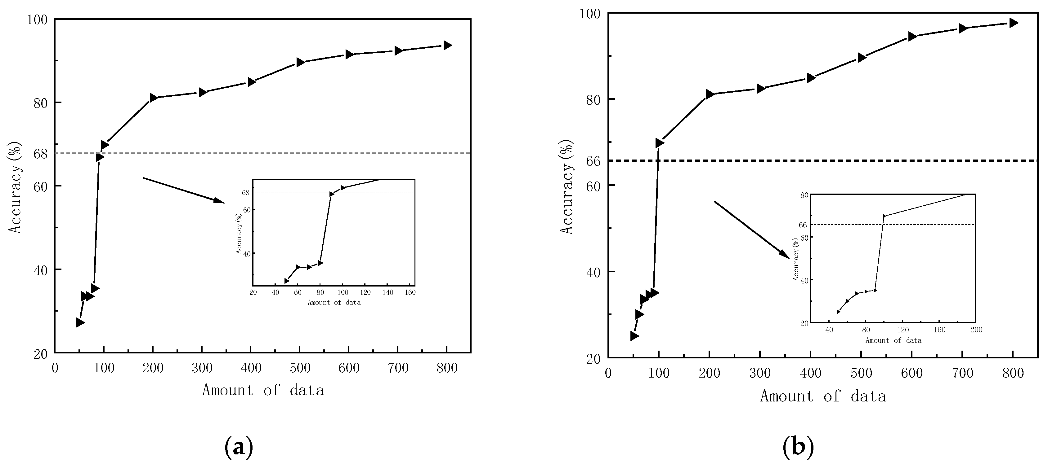
5.3.1. Comparison of the Effect of the Amount of Data in the Target Domain

In order to validate the ability of the proposed transfer-learning-based self-provisioning power risk identification scheme to identify samples from the target domain, the model’s effect is evaluated using different amounts of data from the target domain, and the results are as follows.

The dashed lines in Figure 11 indicate that the average accuracy of the CBAM-CNN fault line selection and power identification models trained on the source domain data is 68% and 66%, respectively, which occurs around a horizontal coordinate of 100. After training the models with a certain amount of target domain data, the accuracy of the models increases with the amount of data. When the amount of data in the target domain is less than 100, the accuracy of the model is less than the average, indicating a negative migration. When the amount of data in the target domain is greater than 100, the accuracy of the model is greater than the average and the accuracy is increased.

5.3.2. Comparison of the Results of Different Risk Identification Schemes

In order to verify the effectiveness of the transfer learning risk identification model proposed in this paper, based on the CBAM-CNN fault routing and self-provisioning power identification model, the transfer method and no transfer method are used to make comparisons respectively, and the results are shown in Figure 12.

The recognition effect of the model can be improved by using the CBAM-CNN model for transfer learning, which takes the model parameters in the original scene as the initial parameters, uses some of the samples in the new scene as the training set, freezes the hidden layer, and fine-tunes the parameters of the fully connected layer. From the above two figures, it can be seen that the proposed transfer learning method in this paper can make the proposed model maintain a high recognition accuracy even with fewer samples.

The following

Table 7. Comparison of the effects of different scheme models.

Scheme	Model	Transfer Scheme	Fault Line Accuracy (%)	Power Supply Identification Accuracy (%)	Accuracy of Power Supply Risk Identification (%)
1	CBAM-CNN	Yes	98.78	99.35	98.78
		No	69.73	66.78	66.78
2	CNN	Yes	89.02	90.02	89.02
		No	65.87	70.35	65.87
3	KNN	Yes	85.64	82.34	82.34
		No	63.41	64.87	63.41
4	DNN	Yes	82.13	86.57	82.13
		No	61.47	63.87	61.47

shows the comparison of the effects of different fault line selection schemes and self-provided power supply identification schemes in the target domain. The accuracy of power supply risk identification is defined as the minimum value of fault line identification accuracy and power supply identification accuracy.

The model proposed in this paper can be used in practice to transfer the model trained in the source domain to the target domain with only a small number of actual fault samples, which can be applied to the risk identification under actual small fault samples and maintain a high accuracy rate.

6. Conclusions

In this study, in order to high accuracy recognition and feature extraction efficiency, we propose a combination of a CBAM and CNN, which achieves automatic extraction of fault risk features by the CNN and enhances the extraction of local features by using the CBAM, so as to achieve high-efficiency feature extraction as well as high-accuracy risk recognition. Due to the small number of fault samples in distribution networks in practice, this paper proposes a transfer-learning-based risk identification method for multiple captive power supplies in active distribution networks, which effectively solves the problem of low accuracy of risk identification in the case of small samples. It is carried out with other modeling methods in experimental simulation, which proves the effectiveness of the proposed method.

The contribution of study can show power grid maintenance personnel in the maintenance of faulty lines before their timely discovery whether there is still unplanned self-supplied power supply to the line and reduce the probability of electric shock casualties of maintenance personnel in the power system industry. Secondly, most methods require a large number of fault samples and, due to the actual number of faults in the distribution network and fault data obtained, this method can effectively solve the problem of low identification accuracy caused by the reality of small fault samples, reduce the risk of self-supplied power supply, greatly increase the reliability of the power supply, and provide a reliable method for the identification of the risk of power supply in the industry.

The introduction of transfer learning solves the problem of small sample size and provides new ideas for the poor learning effect of data-driven methods in active distribution network power supply risk identification. However, in practical applications, large disturbances such as high winds, heavy rains, and strong thunderstorms often have a great impact on the collected fault signals, which in turn makes the model ineffective in practical applications. Therefore, the subsequent research will further study the methods to improve the model recognition accuracy under large disturbances on the basis of resisting small disturbance signals, so as to better improve the model.

References

1. Sun, X.B. Self-contained generator return to send electricity operator electrocution casualties. Rural. Electr. 2017, 25, 35. [Google Scholar]
2. Ren, T.G.; Bao, Y.Z. Fault routing of small-current grounded lines in distribution networks based on discrete Fourier transform. Autom. Technol. Appl. 2023, 42, 67–70. [Google Scholar]
3. Li, J.L.; Ren, J.Y.; Yuan, H.; Wang, Z.J.; Lei, H.; Zhao, Z.J. Arc-grounding fault routing method for distribution networks based on wavelet analysis. J. Zhengzhou Univ. (Eng. Ed.) 2023, 44, 69–76. [Google Scholar]
4. Xie, Q.; Zheng, Q. Single-phase-to-earth Fault Line Selection Method for Medium-voltage Distribution Network Based on Wavelet Packet Analysis. In Proceedings of the 2022 4th International Academic Exchange Conference on Science and Technology Innovation (IAECST), Guangzhou, China, 9–11 December 2022; pp. 257–261. [Google Scholar]
5. Cai, J.; Zhou, B.; Huang, Y.; Zeng, X.J. A new method of fault routing for resonant grounding system based on S-transform time-frequency characteristics. J. Electr. Power Sci. Technol. 2022, 37, 109–116. [Google Scholar]
6. Liu, Z.; Gao, H.; Luo, S. A Fault Phase and Line Selection Method of Double Circuit Transmission Line on The Same Tower Based on Transient Component. In Proceedings of the 2019 IEEE 8th International Conference on Advanced Power System Automation and Protection (APAP), Xi’an, China, 21–24 October 2019; pp. 1058–1062. [Google Scholar]
7. Ren, H.T.; Zhang, Y. Research on fault line selection of distribution network system based on zero sequence transient current. In Proceedings of the 2020 7th International Forum on Electrical Engineering and Automation (IFEEA), Hefei, China, 25–27 September 2020; pp. 390–394. [Google Scholar]
8. Yin, H.W. Power line fault diagnosis technology based on deep transfer learning. Pop. Electr. 2022, 37, 48–50. [Google Scholar]
9. Albarakati, A.J.; Azeroual, M.; Boujoudar, Y.; EL Iysaouy, L.; Aljarbouh, A.; Tassaddiq, A.; EL Markhi, H. Multi-Agent-Based Fault Location and Cyber-Attack Detection in Distribution System. Energies 2023, 16, 224. [Google Scholar] [CrossRef]
10. Wang, P.; Govindarasu, M. Multi-Agent Based Attack-Resilient System Integrity Protection for Smart Grid. IEEE Trans. Smart Grid 2020, 11, 3447–3456. [Google Scholar] [CrossRef]
11. Azeroual, M.; Boujoudar, Y.; Bhagat, K.; El Iysaouy, L.; Aljarbouh, A.; Knyazkov, A.; Markhi, H.E. Fault location and detection techniques in power distribution systems with distributed generation: Kenitra City (Morocco) as a case study. Electr. Power Syst. Res. 2022, 209, 108026. [Google Scholar] [CrossRef]
12. Fan, Y.; Ma, Z.; Tang, W.; Liang, J.; Xu, P. Using Crested Porcupine Optimizer Algorithm and CNN-LSTM-Attention Model Combined with Deep Learning Methods to Enhance Short-Term Power Forecasting in PV Generation. Energies 2024, 17, 3435. [Google Scholar] [CrossRef]
13. Wang, Z.; Mae, M.; Yamane, T.; Ajisaka, M.; Nakata, T.; Matsuhashi, R. Enhanced Day-Ahead Electricity Price Forecasting Using a Convolutional Neural Network–Long Short-Term Memory Ensemble Learning Approach with Multimodal Data Integration. Energies 2024, 17, 2687. [Google Scholar] [CrossRef]
14. Alhanaf, A.S.; Balik, H.H.; Farsadi, M. Intelligent Fault Detection and Classification Schemes for Smart Grids Based on Deep Neural Networks. Energies 2023, 16, 7680. [Google Scholar] [CrossRef]
15. Molla, J.P.; Dhabliya, D.; Jondhale, S.R.; Arumugam, S.S.; Rajawat, A.S.; Goyal, S.B.; Raboaca, M.S.; Mihaltan, T.C.; Verma, C.; Suciu, G. Energy Efficient Received Signal Strength-Based Target Localization and Tracking Using Support Vector Regression. Energies 2023, 16, 555. [Google Scholar] [CrossRef]
16. Rajawat, A.S.; Goyal, S.B.; Bedi, P.; Constantin, N.B.; Raboaca, M.S.; Verma, C. Cyber-Physical System for Industrial Automation Using Quantum Deep Learning. In Proceedings of the 2022 11th International Conference on System Modeling & Advancement in Research Trends (SMART), Moradabad, India, 16–17 December 2022; pp. 897–903. [Google Scholar]
17. Dai, L.; Wang, H. An Improved WOA (Whale Optimization Algorithm)-Based CNN-BIGRU-CBAM Model and Its Application to Short-Term Power Load Forecasting. Energies 2024, 17, 2559. [Google Scholar] [CrossRef]
18. Xiao, C. Research on single-phase ground fault routing in distribution network based on KNN algorithm. J. Nanjing Norm. Univ. (Eng. Technol. Ed.) 2020, 20, 27–31. [Google Scholar]
19. Hao, S.; Zhang, X.; Ma, R.Z.; Wen, H.; Ma, X.; An, B.Y.; Li, J.H. Fault routing method for small current grounding system based on improved GoogLe Net. Grid Technol. 2022, 46, 361–368. [Google Scholar]
20. Zhang, G.D.; Pu, H.T.; Liu, K. Deep learning based fault routing method for small current grounding system. Power Gener. Technol. 2019, 40, 548–554. [Google Scholar]
21. Zhang, D.H.; Zhang, X.W.; Sun, H.; He, J.H. Fault diagnosis of AC/DC transmission system based on convolutional neural network. Power Syst. Autom. 2022, 46, 132–145. [Google Scholar]
22. Yin, H.R.; Miao, S.H.; Guo, S.Y.; Han, J.; Wang, Z.X. A new method for single-phase ground fault routing in distribution networks based on S-transform correlation and deep learning. Power Autom. Equip. 2021, 41, 88–96. [Google Scholar]
23. Pan, S.J.; Yang, Q. A survey on transfer learning. IEEE Trans. Knowl. Data Eng. 2010, 22, 1345–1359. [Google Scholar] [CrossRef]
24. Huang, Z.P.; Zhang, F.Y.; Zhao, J.M.; Jin, Q. A review of transfer learning issues in emotion recognition. Signal Process. 2023, 39, 588–615. [Google Scholar]
25. Zhou, F.Y.; Jin, L.P.; Dong, J. A review of convolutional neural network research. J. Comput. 2017, 40, 1229–1251. [Google Scholar]
26. Wang, Y.F. Research on Fault Routing Method Based on Convolutional Neural Network; Zhengzhou University: Zhengzhou, China, 2021. [Google Scholar]
27. Xie, L.M.; Huang, C.B. A residual network of water scene recognition based on optimized inception module and convolutional block attention module. In Proceedings of the 2019 6th International Conference on Systems and Informatics (ICSAl), Shanghai, China, 2–4 November 2019. [Google Scholar]
28. Sun, Y.F. Research on Adaptive Route Selection Method for Single-Phase Ground Fault in 10 kV Distribution Network; Shenyang Agricultural University: Shenyang, China, 2023. [Google Scholar]
29. Wang, Y.Y.; Chen, Q.S.; Zeng, X.J. Faulty Feeder Detection Based on Space Relative Distance for Compensated Distribution Network with IIDG Injections. IEEE Trans. Power Deliv. 2021, 36, 2459–2466. [Google Scholar] [CrossRef]
Figure 1. Structure diagram of transfer learning.
Energies 17 04438 g001
Figure 2. Pre-training model flowchart.
Energies 17 04438 g002
Figure 3. CNN model transfer training schematic.
Energies 17 04438 g003
Figure 4. Structure of Convolutional Neural Network.
Energies 17 04438 g004
Figure 5. Structure of convolutional block attention module network.
Energies 17 04438 g005
Figure 6. Structure of convolution neural network model with convolutional block attention module network.
Energies 17 04438 g006
Figure 7. Flowchart of power supply risk identification based on transfer learning.
Energies 17 04438 g007
Figure 8. Structure of 10 kV distribution network.
Energies 17 04438 g008
Figure 9. Comparison of fault line selection identification results. (a) Comparison of accuracy; (b) Comparison of loss.
Energies 17 04438 g009
Figure 10. Comparison of power supply identification results. (a) Comparison of accuracy; (b) Comparison of loss.
Energies 17 04438 g010
Figure 11. Comparison of power supply risk identification effects using different target domain data volumes. (a) Fault line selection; (b) Power supply identification.
Energies 17 04438 g011
Figure 12. Comparison of the effects of the with/without transfer learning schemes. (a) Fault line selection; (b) Power supply identification.
Energies 17 04438 g012