The Application of the Particle Element Method in Tubular Propellant Charge Structure: Lumped Element Method and Multiple-Element Method

Abstract

Due to the orderly arrangement of tubular propellant, the permeability of combustion gases is improved, which is beneficial for enhancing the safety of the combustion system. However, current internal ballistic gas-solid flow calculation methods adopt a quasi-fluid assumption, which cannot accurately account for the characteristics of long tube shapes. Additionally, tubular propellants exhibit both overall movement and parameter distribution characteristics, necessitating the decoupling of gas and solid phases. These two deficiencies in previous studies have limited the effectiveness of gas-solid flow simulations for tubular propellant. This paper proposes a numerical calculation model suitable for tubular propellant charging based on the particle element method for internal ballistic two-phase flow. Firstly, considering the overall movement characteristics of tubular propellants, the concept of blank particle elements is introduced to represent pure gas phase regions. Then, based on computational requirements, the tubular propellants are divided to form the lumped element method and the multiple-element method. The moving boundary method is used to calculate the movement process of the propellant bed particle group and is compared with experimental results to verify the applicability of the two methods in tubular propellant beds. Analysis results show that the particle element method can effectively capture changes in the flow field inside the chamber and the position of tubular propellants. The lumped element method can quickly obtain the flow field distribution characteristics inside the chamber, while the multiple-element method can capture parameter distribution characteristics at different positions of the tubular propellants while ensuring overall movement.

1. Introduction

Tubular propellants are widely utilized in combustion systems with large length-to-diameter ratios due to their excellent ventilation and sequential charging characteristics, which ensure operational stability and safety [1,2,3]. These tubular propellants possess an elongated axis and directionality, making their flow, mixing, heat transfer, and interactions with fluids highly complex. Experimental studies indicate that tubular propellants exhibit significantly lower interphase resistance compared to granular particles, particularly when the void fraction is below 0.6. For tubular particles of the same height, interphase resistance ranges from only 2% to 6% of that observed in granular particles [4,5,6].

The traditional lumped parameter algorithms consider the propellant burning inside the chamber under a simultaneous average pressure and are thus unable to obtain the flow field distribution along the axial position inside the chamber, only yielding an average pressure. The pseudo-fluid hypothesis regards particles as a fluid, but such assumptions are only valid in cases of dense and uniformly distributed particles. However, in the case of tubular propellant charging in the chamber, noticeable discontinuities are formed internally, which do not conform to the fluid assumption. Moreover, this assumption fails to capture the shape characteristics of long tubular propellants [7,8]. Therefore, the method of bolt-column flow or porous medium hypothesis is proposed. However, these methods treat the tubular propellant as a whole and cannot capture the changing states of the tubular propellant at different locations. In order to maximize the conformity of the model with the practice and the wide range of parameters, and to simplify the modeling process, it is very important to construct a precise simulation method of tubular propellant combustion flow [9,10]. Therefore, to achieve this goal, two key issues should be addressed. One is to abstract the specific characteristics of tubular particles and model them, and the other is to adapt the existing methods.

Several methods have been proposed to replicate the complex physical processes within the bore and are widely used in internal ballistic computations. Specifically, in the dual-fluid research direction, a universal NOVA code has been developed [11], and similarly, countries like the USA, Germany, and France have developed codes such as EDLTA, EMI, MOBIDIC, TDNOVA, and XNOVAKTC [11,12,13,14]. These codes have formed two-dimensional models of two-phase flow in internal ballistics and have successfully simulated the internal ballistic processes of various granular and tubular propellant charges, accurately predicting the ballistic performance of the charges. The CFD-DEM (Computational Fluid Dynamics-Discrete Element Method) approach has been recognized by many researchers as an effective method for studying two-phase flow under different conditions [15,16,17,18]. In the field of two-phase flow in internal ballistics, Cheng Cheng utilized the CFD-DEM method to investigate ignition behaviors on a microscopic scale [19]. However, due to the high computational cost, CFD-DEM is limited to studying processes within small-scale reactors. In real granular systems, the number of particles can reach trillions, posing a significant challenge for particle element numerical computations on an engineering scale. To improve computational efficiency, coarse-graining methods have been proposed and developed. These methods have been extended to study multicomponent particle separation, heat transfer, and chemical reaction processes [20,21]. These methods mainly focus on particles, and further refinement is needed for tubular or rod-shaped structures.

To overcome the defects in tubular propellant charge modeling, a numerical calculation model suitable for tubular propellant charging based on the particle element method for internal ballistic two-phase flow is proposed [22,23,24]. Firstly, considering the overall movement characteristics of tubular propellants, the concept of blank particle elements is introduced to represent pure gas phase regions. Then, according to computational requirements, the tubular propellants are divided, forming the lumped element method and the multiple-element method, and a particle element solver is constructed. Finally, the particle element solver and CFD solver exchange parameters and update particle element and flow field information. The feasibility of applying the particle element method in tubular propellant charging structures is analyzed, further extending the application scope of the particle element method.

2. Lumped Element Method and Multiple-Element Method

2.1. Physical Model

The study focuses on the gas-solid two-phase reaction flow laws during the firing process of a gun with a fully charging tubular propellant, utilizing the two-phase flow particle element method. The tubular propellant charge structure is illustrated in Figure 1. The entire firing process can be described as follows: High-temperature gas generated by the primer interacts with the incandescent solid particles, igniting the tubular propellant. Subsequently, the flame rapidly propagates and ignites the entire propellant bed. The high-temperature and high-pressure combustion gases overcome the resistance of the projectile, propelling it forward until it is ejected from the muzzle.

Based on the physical processes, the following assumptions are made for facilitating the modeling and computation of the two-phase flow of tubular propellant:

(1)

Each tubular propellant within the same bundle shares identical shape, dimensions, and properties, with identical combustion and motion laws.

(2)

Surface ignition temperature criterion is adopted for the tubular propellant, ensuring simultaneous ignition inside and outside the tube on the same cross-section.

(3)

The tubular propellants are treated as incompressible.

(4)

The thermodynamic characteristics of the propellant gas remain constant and adhere to the Nobel–Abel state equation.

(5)

The flow in the chamber is assumed to be inviscid.

The chamber is not assumed to have a continuous distribution, as in the case of particle charges, but axial bundles of non-interconnected bundles. Therefore, it is necessary to further supplement the particle element method to adapt to the tubular propellant charging situation. In this paper, the lumped element model based on the tubular propellant movement model and the multiple-element model based on the granular drug hypothesis are proposed.

2.2. Particle Element Method

The specific partitioning and motion method of particle elements is detailed in the author’s earlier publication on the particle elements method [22,23,24]. This paper mainly discusses the extended application of this method in tubular propellant, which can be divided into two categories: lumped element method and multiple-element method.

2.2.1. Lumped Element Method

In the lumped element model, when partitioning the particle elements, the tubular propellant bundles are divided into fixed-size elements, with each tubular propellant particle element length being consistent with the length of the propellant bundle. The remaining regions are separately partitioned as blank elements to connect the particle elements in the tubular propellant section, ensuring that the chamber interior maintains a continuous distribution of elements, as illustrated in Figure 2.

From the perspective of tubular propellant charging characteristics, tubular propellant does not possess good dispersal properties like granular propellant. Therefore, there is no solid phase distribution in the blank areas formed before and after motion. As a result, a separate blank particle element is left between the chamber bottom, projectile base, and propellant bundle to ensure that the tubular propellant does not exceed the limits of the chamber bottom, projectile base, and each other. The blank particle element only contains the distribution of the gas phase flow field, does not undergo motion itself, and does not generate gas. Its size changes only due to the boundary changes in the motion of the tubular propellant particle elements.

The motion of tubular propellant can be described by the variable mass form of Newton’s second law, considering the effects of pressure gradient and interphase forces:

$${\displaystyle \frac{d}{dt}}{\displaystyle {\int }_{x_L}^{x_R}\left(1-\varphi \right){\rho }_p{u}_{p}Adx=}-{\displaystyle {\int }_{x_L}^{x_R}\left(1-\varphi \right)Adp-}{\displaystyle {\int }_{x_L}^{x_R}{m}_c{u}_{p}Adx+{\displaystyle {\int }_{x_L}^{x_R}A{f}_{s}dx}}$$

(1)

$${\displaystyle \frac{dx}{dt}}=u_p$$

(2)

After the motion of the tubular propellant bundle, when adjusting the positions of the particle elements, it is essential to use the center of mass position of the first tubular propellant bundle closest to the chamber bottom as the reference point. Based on the length of the tubular propellant, the left and right boundaries of the particle elements are determined, followed by sequentially determining the positions of the particle elements for subsequent tubular propellant bundles. Finally, the size of the blank particle element is determined, and position adjustments are made accordingly.

2.2.2. Multiple-Element Method

Unlike the lumped element model, the multiple-element model divides the tubular propellant into segments of a certain length in accordance with the intent of the particle element model itself. In terms of motion, the tubular propellant is artificially divided into several bundles of small particle elements, which are interconnected, as shown in Figure 3. During combustion calculations, the particles are still computed according to the shape function of the tubular propellant, with the combustion source terms released within the particle elements.

The multiple-element model can be used to calculate the tubular propellant more carefully, addressing the issue of oversized particle elements caused by excessively long propellant rods, which can compromise computational accuracy. In the analysis of tubular propellant without grooving, the rupture location can be paid attention to in real time to analyze the rupture law of tubular propellant. It is also suitable for the mixed charge model, which is helpful for the unified modeling of mixed charges. However, in order to ensure the rationality of particle movement, the particle elements of tubular propellant need to be further restricted.

With reference to the particle element method [22,23,24], the motion equation of particles can be provided as follows:

$${\displaystyle \frac{d{u}_p}{dt}}={\displaystyle \frac{f_s+\delta p+R_p}{M}}$$

(3)

Since the multiple elements are only artificially divided, in reality, the tubular propellant bundle moves at the same speed everywhere. Therefore, after calculating the motion of each particle element, a uniform velocity can be obtained for the whole population of particle elements belonging to the same drug bundle according to the conservation of momentum:

$$Mv={\displaystyle \sum _{i=1}^{NKL}{u}_p{m}_p}$$

(4)

Each particle element within each tubular propellant moves according to this velocity, resolving the internal boundary constraints.

2.3. Gas Phase Flow Field Equation

In the gas phase flow field, the continuum hypothesis is still adopted. The gas phase control equations in the chamber are written in vector form as follows:

$${\displaystyle \frac{\partial U}{\partial t}}+{\displaystyle \frac{\partial F}{\partial x}}=H$$

(5)

where $U=\left(\begin{array}{l}\varphi {\rho }_g\\ \varphi {\rho }_g{u}_g\\ \varphi {\rho }_g(e_g+u_g^2/2)\end{array}\right)$, $F=\left(\begin{array}{l}\varphi u_g{\rho }_g\\ \varphi \left({\rho }_g{u}_g^2+p\right)\\ \varphi u_g\left[{\rho }_g(e_g+u_g^2/2)+p\right]\end{array}\right)$, $H=\left(\begin{array}{l}{m}_c+m_{ign}\\ -f_s+m_c{u}_p+p{\displaystyle \frac{\partial \varphi }{\partial x}}+m_{ign}{u}_{ign}\\ -f_s{u}_p-Q_p-p{\displaystyle \frac{\partial \varphi }{\partial t}}+m_c{H}_p+m_{ign}{H}_{ign}\end{array}\right)$.

2.4. Auxiliary Equation

The specific auxiliary equations can be found in ref. [8]. However, because the properties of tubular propellants are very different from those of granular, the corresponding combustion equations and inter-phase resistance equations are different from those described above.

(1)

Inter-phase resistance equation of tubular propellant.

The relationship for the inter-granular resistance of tubular propellant, which is much smaller than that of granular packed propellant beds due to the orderly arrangement and good permeability, can be expressed as:

$$f_s={\displaystyle \frac{(1-\varphi )}{d_p}}\left|u_g-u_p\right|(u_g-u_p){\rho }_g{C}_f$$

(6)

$$C_f=\left\{\begin{array}{ll}0.17& \hspace{1em}\hspace{1em}\varphi \le 0.6\\ 0.17-0.152\ast {\displaystyle \frac{\varphi -0.6}{0.2}}& \hspace{1em}\hspace{1em}0.6<\varphi \le 0.8\\ 0.018& \hspace{1em}\hspace{1em}0.8<\varphi \le 1\end{array}\right.$$

(7)

(2)

Combustion equation of tubular propellant.

The tubular propellant charge bundle is burned according to the geometric combustion law, and the burning rate equation adopts the exponential formula, namely

$$\begin{array}{l}{r}_e=r_{e0}-{\displaystyle \int u_1{p}^{n}dt}\\ r_i=r_{i0}+{\displaystyle \int u_1{p}^{n}dt}\end{array}$$

(8)

In the formula, r_e0 and r_i0 are the initial outside diameter and inside diameter of a single tubular propellant, respectively. r_e and r_i are the outer diameter and inner diameter of tubular propellant at any time, respectively. u₁ and n are the burning rate coefficient and burning rate index of tubular propellant charge, respectively. The burned mass at any time is

$$m_c={\displaystyle \sum _N{\rho }_p\pi c_1\left[\left(r_{e0}^2-r_{i0}^2\right)-\left(r_e^2-r_i^2\right)\right]}$$

(9)

2.5. Coupling and Parameter Transfer between Particle Elements and Flow Field Grid Cells

Particle elements need to transfer source terms and couple calculations with the flow field. Depending on the size of the chamber volume and calculation requirements, the flow field domain grid inside the chamber is divided, with the fluid domain grid taking dx as the grid cell length. By using overlapping grid technology, the fluid grid overlaps with the particle elements, where the flow field grid is a Eulerian grid and the particle elements move on the flow field grid. Based on the combustion state of the corresponding particle element at the respective position in the flow field domain, the flow field computation source terms are updated, and flow field solving is performed. The entire process is divided into two phases:

(1)

Flow field computation.

In the flow field computation phase, the parameters required include initial parameters of the flow field and particle parameters. The initial parameters of the flow field are determined by the initial flow field state, including temperature, pressure, and gas phase velocity, where the finishing state of the previous time step serves as the initial parameters for the next time step’s flow field calculation. The particle parameters are determined by the particle element parameters corresponding to the current gas phase grid, with the current positions, shapes, velocities, and energies of the particle elements used to calculate their impact on the flow field for subsequent auxiliary equation calculations. These parameters are then incorporated into the flow field calculations in the form of source terms and allocated to the respective flow field grid.

(2)

Particle element computation.

In the particle element computation phase, the movement and combustion of the particle elements need to be calculated. Forces and motion of the particle elements are calculated based on the corresponding flow field parameters such as pressure, gas phase flow velocity, and the shape of particles inside the particle element. The source terms for particle combustion and shape changes are determined based on the pressure and temperature within the flow field, to obtain a set of particle element parameters.

3. Numerical Calculation Method

3.1. Numerical Method

The semi-discrete equation after discretizing the spatial derivative of Equation (5) is as follows:

$${\displaystyle \frac{\partial U}{\partial t}}=Q_n+R_n$$

(10)

where Q_n is the discrete post-space derivative term and R_n is the source term, using the third-order TVD Runge-Kutta method for discretization:

$$\begin{array}{l}{U}^{\left(1\right)}=U^n+\Delta tQ\left(U^n\right)+R_n\\ U^{\left(2\right)}=3/4U^n+1/4U^{\left(1\right)}+1/4\Delta tQ\left(U^{\left(1\right)}\right)+R_n\\ U^{n+1}=1/3U^n+2/3U^{\left(2\right)}+2/3\Delta tQ\left(U^{\left(2\right)}\right)+R_n\end{array}$$

(11)

where ∆t is the time step, it can be determined according to the following formula:

$$\Delta t\le {\displaystyle \frac{CFL\times dx}{{\left|{\lambda }^{\ast }\right|}_{\max }}}$$

(12)

where dx is the grid cell scale and λ* is the global maximum eigenvalue, which can be calculated from the above algorithm.

3.2. Calculation Condition

To validate the effectiveness of the particle element method, the study referenced literature [1] and utilized mature experimental charging conditions as the research subject. The conditions in the chamber at the time of ignition are set as the initial conditions. The gas-solid phase velocity is 0, the pressure is atmospheric pressure, the temperature is the initial propellant temperature, the density is determined using the equation of state, and the porosity is determined based on the charging conditions. The specific parameters of chamber and tubular propellant used are shown in

Table 1. Parameters of chamber and tubular propellant [1].

Parameters	Value	Parameters	Value
Caliber A/mm	50	Ratio of specific heats γ	1.232
Projectile travel l/mm	3195	Powder density ρp/(kg·m−3)	1615
Projectile mass m/kg	2.5	Covolume α/(m3/kg)	0.001
Ignition mass mign/g	4.5	Burn rate index n	0.874
Main charge mass m/kg	0.5	Burn rate coefficient a/(cm·MPa−n·s−1)	0.2299
Detonation temperature/K	3133	Tubular propellant size/mm	Φ 6.35 × 200
powder impetus f/(kJ/kg)	1036	Diameter of chamber/mm	2.20

.

3.3. Mesh Generation

According to the above two particle element methods, two sets of grid systems were divided to calculate the interior trajectory process, as shown in Figure 4 below:

The lumped element method divides the entire tubular propellant charge bundle into one particle element, and both ends correspond to the gas phase grid, and two blank particle elements are divided into the bottom of the chamber and the bottom of the projectile. The multiple-element method further divides the tubular propellant particle elements to form the particle elements excluding the blank particle elements. And the boundary of the particle elements corresponds to the boundary of the gas phase grid. The common feature for these two methods is that the gas phase mesh and the blank particle elements before and after are the same, and the difference is that the particle elements of the tubular propellant are divided.

3.4. Calculation Process

The calculation process of tubular propellant particle element method is shown in Figure 5. When the tubular propellant charging is initially divided into particle elements, the multiple-element method or the lumped element method can be selected according to the needs. After the particle element is divided, the particle element solver and CFD solver are used, respectively, to solve the particle element and flow field until the calculation-terminating condition is reached.

The influence of the grid refinement has been investigated with four grids of the particle element method shown in Figure 6. The scale of the four groups of grids is 10.0 mm, 5.0 mm, 2.5 mm, and 1.0 mm, respectively, and the flow field parameters of the four groups of grids are obtained and compared. When the grid scale is less than 2.5 mm, the grid is fine enough to produce numerically accurate results.

4. Results and Discussion

4.1. Comparison of Experimental and Numerical Simulation Results

Figure 7 presents a comparison of the chamber bottom pressure curves obtained from simulations using the lumped element method and the empty particle element method, with the experimental pressure curve. It can be observed from the graph that the calculated results are in good agreement with the experimental data. Therefore, the simulation codes for both methods can effectively predict the internal ballistics performance of tubular propellant. In the initial stage of internal ballistics, there is a certain degree of error between the simulated calculation and the experimental testing due to factors such as the assumptions used in the ignition process in the simulation.

In the later stages of internal ballistics, the lumped element method exhibits some error in pressure compared to experiments due to the relatively large size of the particle elements, resulting in less precise capture of chamber pressure. Conversely, the multiple-element method maintains higher accuracy, closely matching experimental pressure curves. Figure 8 compares velocity curves calculated by both methods with experimental data. It demonstrates that both sets of curves align closely with experimental results, with pressure calculation errors below 5%, further confirming the accuracy of both methods.

4.2. Analysis of the Tubular Propellant Movement

To further investigate the differences between the two calculation methods, Figure 9a,b present trajectory curves of the tubular propellant computed using the two methods. The red and black curves in the figures represent the variations in the positions of the left and right ends over time. It is observed from the graphs that the displacement of the tubular propellant is minimal, remaining predominantly within the chamber during firing, with a maximum displacement of approximately 7 mm. Both methods yield final displacements of around 5 mm, demonstrating highly consistent motion characteristics.

The velocity of the tubular propellant is also quite similar, as shown in Figure 10a,b. Due to the fluctuation in chamber pressure, the tubular propellant oscillates back and forth within the chamber. However, the velocity is relatively low, with a maximum speed not exceeding 9 m/s. Eventually, the velocity of the tubular propellant gradually decreases to 0, at which point the propellant grain remains in position until completely burned out.

The particle element method provides a visual representation of particle motion and void fraction distribution. Figure 11 illustrates a particle distribution calculated using the multiple-element method. The entire tubular propellant is represented as multiple equivalent particles, with each sphere’s diameter representing the length of an equivalent particle. The color filling inside indicates the current porosity of each equivalent particle. The horizontal axis denotes time, while the vertical axis represents the current position of the particles.

When studying the distribution characteristics of particles inside the chamber, we employed different sizes of particle element division scales (5 mm, 4 mm, 2 mm, and 1 mm), corresponding to 4, 5, 10, and 20 particle elements within the chamber. By comparing the data in Figure 12, it is evident that finer particle element divisions lead to richer distribution details: as the size of particle elements decreases (i.e., the number of particle elements increases), we are able to capture more detailed particle distribution information. This indicates that refining the division of particle elements contributes to enhancing the accuracy of the model. The overall data distribution remains consistent: despite the varying degrees of particle element division, the data distribution under different particle element divisions, as indicated by the average parameters in the yellow dashed box in the figure, does not show significant differences. This suggests that, overall, the size of particle elements has a minor impact on data distribution trends. In cases where high precision is not required, simulations and calculations can be performed with fewer particle elements to reduce computational resource consumption and improve efficiency. For scenarios involving key parameters or requiring the capture of more detailed distributions, a finer division of particle elements should be utilized to ensure the accuracy of analysis results. In practical applications, the division scale of particle elements should be flexibly adjusted based on research objectives and actual needs to achieve optimal analytical outcomes.

From the graph, it is evident that during the initial phase, the motion of the tubular propellant is minimal, and the blank particle element at the base of the chamber is nearly imperceptible. As the tubular propellant moves, a void space gradually emerges at the base of the chamber, and the blank particle element at the base is progressively enlarged, as indicated by the red dashed line box in the diagram. Utilizing the multiple-element method, it is possible to capture the variations in each small region of the propellant grain and reflect them in the particles. Furthermore, during the computational process, it is feasible to simulate fragmentation and transformation based on actual conditions, which necessitates further research. The length of the effective particles within the chamber always remains consistent with the length of the propellant grain.

The parameter distribution diagram calculated using the lumped element method is shown in Figure 13. Unlike the multiple-element method, the tubular propellant is directly modeled as a “plug” in this approach, which more intuitively demonstrates the high length-to-diameter ratio characteristic of the tubular propellant. The motion pattern of the propellant remains consistent with the above description, as the tubular propellant moves forward as a whole. Additionally, as the propellant advances, the blank particle element at the base of the chamber gradually elongates as shown in Figure 14. As the combustion progresses, the porosity of the tubular propellant within the chamber increases gradually, while the porosity of the blank particle element remains constant at 1.

4.3. Analysis of Flow Field

The flow field within the chamber is crucial for accurately applying the particle method. It was previously demonstrated that the calculation differences between the two methods are minimal, so this section only analyzes the multiple-element method. Figure 15 shows the axial pressure distribution within the chamber from 1 ms to 4 ms. Due to the shape of the tubular propellant, there is a significant free space at the base of the chamber during charging. Therefore, it can be observed that the pressure within the tubular propellant region remains relatively uniform during the initial 1–4 ms, indicating good flame propagation. However, the pressure in the cylindrical propellant region is significantly higher than that in the void space at the base, resulting in a noticeable pressure drop at their interface. This is due to the large free space in the void area, leading to gas expansion.

Figure 16 shows the distribution of pressure in the chamber along the axis from 6 ms to 14 ms. It can be seen from the figure that the pressure in the chamber always presents a certain drop at the front and back ends of the tubular propellant before the end of combustion. Because of the good permeability of the tubular propellant, the motion velocity is much lower than the gas flow speed, so the bottom pressure is always less than the bottom pressure. When the tubular cylinder gradually burns out, the pressure in the chamber tends to be stable, and the pressure in the whole chamber is nearly uniform.

The superficial gas velocities distribution and density distribution within the chamber are shown in Figure 17 and Figure 18, respectively. In the initial stages, the combustion gases propagate rapidly along the axial direction of the chamber. Upon reaching the projectile base and chamber base, they are reflected by the solid wall boundaries, creating oscillatory regions between the projectile base and chamber base. Due to the porous structure leading to low flow velocity, higher velocities can be achieved in free space, resulting in a significant contrast between the left and right boundaries at the interface inside the chamber. The movement of the projectile causes continual expansion of the chamber space, resulting in a gas velocity distribution where the velocity is higher at the projectile base than at the chamber base, extending until the projectile exits the muzzle. The density distribution within the chamber also exhibits interruptions at the interface between the propellant region and the void space. However, due to gas accumulation at the projectile base, the gas density at the projectile base remains higher than at other locations within the chamber.

Based on the above analysis, the lumped element method and the multiple-element method are adopted after the blank particle element is introduced into the particle element method. Both methods can be applied to calculate two-phase flow in the internal ballistics of tubular propellant charge structures, and accurately predict the development of tubular propellant charge motion and flow field.

5. Conclusions

This research focuses on the structure of a tubular propellant charge, proposing the concept of blank particle elements and developing both the lumped element method and the multiple-element method. Applications to practical numerical examples indicate that results from both methods are in good agreement with experiment, effectively capturing variations in the flow field inside the chamber and the position of the tubular propellant. This confirms the applicability of the particle element method in tubular propellant beds. The specific conclusions are as follows:

(1)

The multiple-element method has high accuracy and can be highly consistent with the test curve. However, the lumped element is large, and the pressure capture in the chamber is not fine enough, which leads to a certain error between the lumped element method and the test.

(2)

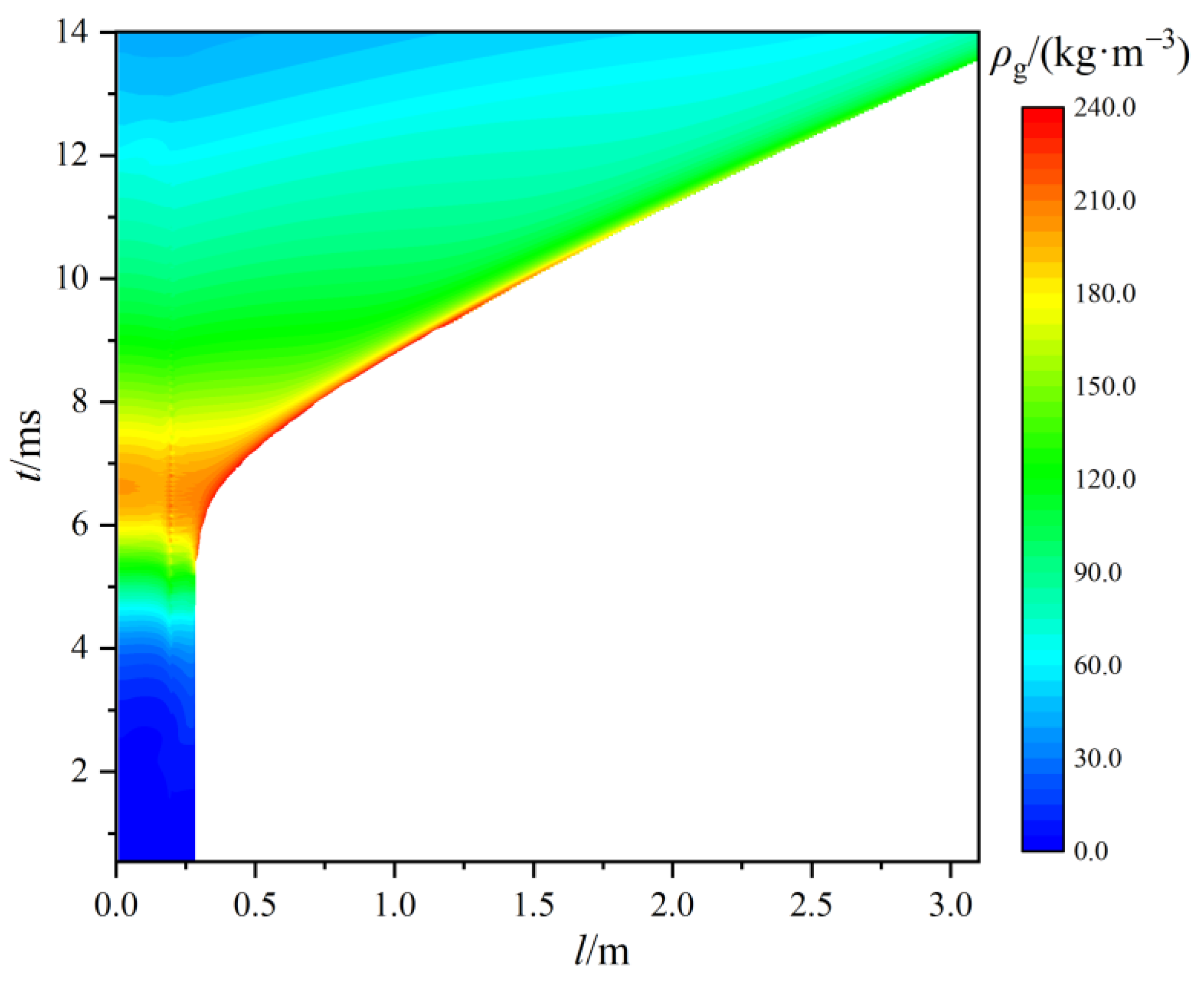
The tubular propellant bundle vibrates back and forth in the chamber, but the speed is relatively small, the maximum speed is not more than 8 m/s, in the initial period, the movement of the bundle is very small, and the blank particle element at the bottom of the chamber is almost invisible. With the movement of the tubular bundle, the void space gradually appeared in the bottom of the chamber, and the blank particle element in the bottom of the chamber gradually expanded.

(3)

The free space causes the gas to expand easily, and the pressure in the propellant region is significantly higher than that in the free region, resulting in an obvious interfacial pressure gap. Fluid flows through the solid particle bed due to the porous structure, resulting in low flow rate. While free space flow rate distribution is relatively uniform, the fluid in free space can reach higher speeds.

References

1. Miura, H.; Matsuo, A.; Nakamura, Y. Numerical Prediction of Interior Ballistics Performance of Projectile Accelerator Using Granular or Tubular Solid Propellant. Propellants Explos. Pyrotech. 2013, 38, 204–213. [Google Scholar] [CrossRef]
2. Woodley, C.; Carriere, A.; Franco, P.; Gröger, T.; Hensel, D.; Nussbaum, J.; Kelzenberg, S.; Longuet, B. Comparisons of internal ballistics simulations of the AGARD gun. In Proceedings of the 22nd International Symposium on Ballistics, Vancouver, BC, Canada, 14–18 November 2005; Volume 1, pp. 339–345. [Google Scholar]
3. Jang, J.; Oh, S.; Roh, T. Comparison of the characteristics of granular propellant movement in interior ballistics based on the interphase drag model. J. Mech. Sci. Technol. 2014, 28, 4547–4553. [Google Scholar] [CrossRef]
4. Xiao, Z.; Xu, F. Relationship between slivering point and gas generation rules of 19-perforation TEGDN propellants with different length/outside diameter ratios and perforation diameters. J. Energetic Mater. 2016, 36, 141–151. [Google Scholar] [CrossRef]
5. El Sadek, H.; Zhang, X.; Rashad, M. Interior ballistic study with different tools. Int. J. Heat Technol. 2014, 32, 141e6. [Google Scholar]
6. Cheng, S.; Jiang, K.; Xue, S.; Tao, R.; Lu, X. Performance analysis of internal ballistic multiphase flow of composite charge structure. Energies 2023, 16, 2127. [Google Scholar] [CrossRef]
7. López-Munoz, C.; García-Cascales, J.; Velasco, F.; Otón-Martínez, R. An Energetic Model for Detonation of Granulated Solid Propellants. Energies 2019, 12, 4459. [Google Scholar] [CrossRef]
8. Xue, X.; Ye, Q.; Yu, Y. Three-dimensional heat transfer characteristics of complex structure with nineteen tubular propellants under different heating rates. Int. Commun. Heat Mass Transf. 2022, 139, 106491. [Google Scholar] [CrossRef]
9. Ongaro, F.; Robbe, C.; Papy, A.; Stirbu, B.; Chabotier, A. Modelling of internal ballistics of gun systems: A review. Def. Technol. 2024; in press. [Google Scholar] [CrossRef]
10. Otón-Martínez, R.A.; Velasco, F.J.; Nicolás-Pérez, F.; García-Cascales, J.R.; Mur-Sanz de Galdeano, R. Three-Dimensional Numerical Modeling of Internal Ballistics for Solid Propellant Combinations. Mathematics 2021, 9, 2714. [Google Scholar] [CrossRef]
11. Gough, P.S.; Zwarts, F.J. Modeling Heterogeneous Two-Phase Reacting Flow. AIAA J. 1979, 17, 17–25. [Google Scholar] [CrossRef]
12. Gough, P.S. Some Fundamental Aspects of the Digital Simulation of Convective Burning in Porous Beds; AIAA: Orlando, FL, USA, 1977; pp. 77–855. [Google Scholar]
13. Gough, P.S. Formulation of a Next-Generation Interior Ballistic Code; PGA-TR-91-3; Paul Gough Associates: Portsmouth, UK, 1993. [Google Scholar]
14. Gough, P.S. Modeling arbitrarily packaged multi-increment solid propellant charges of various propellant configurations. In Proceedings of the 33rd JANNAF Combustion Meeting, Monterey, CA, USA, 4–8 November 1996; CPIA Publication: Washington, DC, USA, 1996; pp. 421–435. [Google Scholar]
15. Ma, H.; Zhao, Y.; Cheng, Y. CFD-DEM modeling of rod-like particles in a fluidized bed with complex geometry. Powder Technol. 2019, 344, 673–683. [Google Scholar] [CrossRef]
16. Yao, L.; Liu, Y.; Liu, J.; Xiao, Z.; Xie, K.; Cao, H.; Zhang, H. An optimized CFD-DEM method for particle collision and retention analysis of two-phase flow in a reduced-diameter pipe. Powder Technol. 2022, 405, 117547. [Google Scholar] [CrossRef]
17. Lin, Z.; Sun, X.; Yu, T.; Zhang, Y.; Li, Y.; Zhu, Z. Gas–solid two-phase flow and erosion calculation of gate valve based on the CFD-DEM model. Powder Technol. 2020, 366, 395–407. [Google Scholar] [CrossRef]
18. Hu, C.; Luo, K.; Yang, S.; Wang, S.; Fan, J. A comprehensive numerical investigation on the hydrodynamics and erosion characteristics in a pressurized fluidized bed with dense immersed tube bundles. Chem. Eng. Sci. 2016, 153, 129–145. [Google Scholar] [CrossRef]
19. Cheng, C.; Zhang, X. Numerical Investigation on the Transient Ignition Behavior Using CFD-DEM Approach. Combust. Sci. Technol. 2014, 186, 1115–1137. [Google Scholar] [CrossRef]
20. Lu, L.; Morris, A.; Li, T.; Benyahia, S. Extension of a coarse grained particle method to simulate heat transfer in fluidized beds. Int. J. Heat Mass Transf. 2017, 111, 723–735. [Google Scholar] [CrossRef]
21. Lu, L.; Yoo, K.; Benyahia, S. Coarse-grained-particle method for simulation of liquid–solids reacting flows. Ind. Eng. Chem. Res. 2016, 55, 10477–10491. [Google Scholar] [CrossRef]
22. Cheng, S.; Tao, R.; Xue, S.; Lu, X. The Particle Element Method to Obtain Parameter Distributions of Two-phase Reactive Flow in a Propulsion Combustion System. Combust. Sci. Technol. 2024, 196, 730–752. [Google Scholar] [CrossRef]
23. Cheng, S.; Wang, H.; Xue, S.; Tao, R. Application and Research of the Particle Element Model in Ignition Process of Large-Particle High-Density Charge. Combust. Sci. Technol. 2022, 194, 1850–1871. [Google Scholar] [CrossRef]
24. Cheng, S.; Tao, R.; Lu, X.; Xue, S.; Jiang, K. Efficient two-dimension particle element method of interior ballistic two-phase flow. Combust. Theory Model. 2023, 27, 558–583. [Google Scholar]
Figure 1. Tubular charge structure diagram.
Energies 17 04384 g001
Figure 2. Schematic diagram of lumped element model.
Energies 17 04384 g002
Figure 3. Schematic diagram of multiple-element model.
Energies 17 04384 g003
Figure 4. Diagram of grid division in tubular propellant charge chamber.
Energies 17 04384 g004
Figure 5. Calculation flow chart of tubular propellant particle element method.
Energies 17 04384 g005
Figure 6. The variation of chamber bottom pressure over time at different grid scales.
Energies 17 04384 g006
Figure 7. Comparison of pressure curves by different methods.
Energies 17 04384 g007
Figure 8. Comparison of velocity curves by different methods.
Energies 17 04384 g008
Figure 9. The trajectory of the tubular propellant.
Energies 17 04384 g009
Figure 10. The velocity of the tubular propellant.
Energies 17 04384 g010
Figure 11. Particle elements distribution with the multiple-element method. (a) Distribution status of 2–9 ms (b) 5–7 ms partial view.
Energies 17 04384 g011
Figure 12. Parameter variation of chamber bottom at different particle element scales.
Energies 17 04384 g012
Figure 13. Particle elements distribution with the lumped element method.
Energies 17 04384 g013
Figure 14. Position distribution of blank particle elements.
Energies 17 04384 g014
Figure 15. Pressure distribution along the axis in 1 ms–4 ms.
Energies 17 04384 g015
Figure 16. Pressure distribution along the axis in 6 ms–14 ms.
Energies 17 04384 g016
Figure 17. Gas velocity distribution in the chamber.
Energies 17 04384 g017
Figure 18. Gas density distribution in the chamber.
Energies 17 04384 g018